Single molecule localization by $\ell_{2}-\ell_{0}$ constrained optimization

Abstract

Single Molecule Localization Microscopy (SMLM) enables the acquisition of high-resolution images by alternating between activation of a sparse subset of fluorescent molecules present in a sample and localization. In this work, the localization problem is formulated as a constrained sparse approximation problem which is resolved by rewriting the $\ell_{0}$ pseudo-norm using an auxiliary term. In the preliminary experiments with the simulated ISBI datasets the algorithm yields as good results as the state-of-the-art in high density molecule localization algorithms.

1 Introduction

The exploration of fluorescent molecules in microscopy has made it possible to bypass the limit of resolution imposed by the diffraction limit and obtain images often referred to as super-resolved images (see [5], [3] and [6]). The principle of SMLM is to excite a sparse number of fluorescent molecules for each acquisition and locate each molecule with an algorithm. Since fluorescence microscopy can be used for live imaging, the subject may move during the acquisitions yielding a faulty reconstruction. More molecules excited for each single acquisition will lower the total acquisition time. Therefore the subject has less time to move with high-density acquisition. This demands an efficient reconstruction as more than one molecule could be present in the same diffraction disk.

In this work we aim to reconstruct precisely high-density 2D images. We model the localization problem as a $\ell_{2}-\ell_{0}$ constrained minimization problem. A similar approach, the $\ell_{2}-\ell_{0}$ penalized minimization problem, has been previously studied with success [4]. However, a common problem with penalized regularizations terms is to choose the trade-off parameter between the data fidelity term and the regularization term. In this paper we look at the $\ell_{2}-\ell_{0}$ constrained version as the sparsity parameter is easier to handle. We propose a minimization algorithm based on exact reformulation of the $\ell_{0}$ pseudo-norm by introducing an auxiliary variable.

2 Acquisition system modelling

The fluorescence molecules are observed through an optical system and thus the signal, $x\in\mathbb{R}^{ML\times ML}$, is diffracted. This is modeled by the Point Spread Function (PSF) which is convolved with the signal. This operation is denoted $H:\mathbb{R}^{ML\times ML}\rightarrow\mathbb{R}^{ML\times ML}$, and we have chosen to use the Gaussian approximation of the PSF

$$PSF(x_{1},x_{2})=\frac{1}{\sqrt{2\pi}\sigma_{s}}\exp\left[-\frac{x_{1}^{2}+x_{2}^{2}}{2\sigma_{s}^{2}}\right]$$ (1)

where $\sigma_{s}$ is spatial standard deviation.

A sensor captures the convolved signal in a lower resolution which is modeled by a reduction operator $R_{L}:\mathbb{R}^{ML\times ML}\rightarrow\mathbb{R}^{M\times M}$ which is defined as

$$R_{L}(x)=RXR^{T}$$ (2)

where $X\in\mathbb{R}^{ML}\times\mathbb{R}^{ML}$ and $X$ is the vector $x$ arranged as a matrix. $R$ is a matrix of $\mathbb{R}^{M}\times\mathbb{R}^{ML}$ with $L$ 1’s in each line and $R^{T}$ is the transposed matrix of $R$.

During this image acquisition the signal is corrupted by different kind of noise $\eta$. In this work we assume the noise to be Gaussian additive noise. The system can therefore by modeled as

$$d=R_{L}(H(x))+\eta$$ (3)

with $d\in\mathbb{R}^{M\times M}$ and $x\in\mathbb{R}^{ML\times ML}$. Further on we will refer the linear operation $R_{L}(H(x))=Ax$ to ease the notations.

The localization is done on a finer grid $x\in\mathbb{R}^{ML\times ML},L>1,$ than the observed signal $d\in\mathbb{R}^{M\times M}$. Therefore, the inverse problem is underdetermined. We include a sparse constraint term as only a few number of molecules are excited for each acquisition, and we note the maximum number of molecules we want to reconstruct as $k$ which is the sparsity parameter. This constraint is introduced as $\iota_{\|\cdot\|_{0}\leq k}(x)$, where $\|x\|_{0}=\#\{x_{i},i=1,\cdots N:x_{i}\neq 0\}$, and will be, by abuse of language, referred to as the $\ell_{0}$ norm. $\iota_{C}(x)$ is the indicator function such that

$$\iota_{C}(x)=\begin{cases}0\text{ if }x\in C\\ +\infty\text{ otherwise }\end{cases}$$

Furthermore, we add the constraint that each reconstructed molecule must have a positive value since we reconstruct their intensity. We search therefore

$$\hat{x}\in\operatorname*{arg\,min}_{x\in\mathbb{R}^{ML\times ML}}\frac{1}{2}\|Ax-d\|^{2}+\iota_{\|\cdot\|_{0}\leq k}(x)+\iota_{\cdot\geq 0}(x)$$ (4)

This problem is non-convex and non-continuous as well as NP-hard due to the nature of the $\ell_{0}$ norm. The problem has been extensively studied, and among the approaches to ease or resolve the problem we find relaxations of the $\ell_{0}$ norm [8] and greedy algorithms [9]. In this paper we use an exact reformulation of the $\ell_{0}$ norm that we will present in the next section.

3 Exact reformulation of the $\ell_{0}$ norm

The article [11] inspired us to extend their results to the $\ell_{2}-\ell_{0}$ constrained problem. They propose to rewrite the $\ell_{0}$ norm as a convex minimization problem by introducing an auxiliary variable $u$.

$$\|x\|_{0}=\min_{-1\leq u\leq 1}\|u\|_{1}\text{ s.t }\|x\|_{1}=<u,x>$$ (5)

With the reformulation of the $\ell_{0}$ norm we can rewrite our problem as

$$\min_{x,u}\frac{1}{2}\|Ax-d\|+\iota_{\cdot\geq 0}(x)+I(u)\text{ s.t. }\|x\|_{1}=<x,u>$$

where $I(u)$ is :

$$I(u)=\begin{cases}0\text{ if }\|u\|_{1}\leq k\text{ and }-1\leq u\leq 1\\ \infty\text{ otherwise }\end{cases}$$

We can then define a new penalty term

$$G_{\rho}(x,u)=\frac{1}{2}\|Ax-d\|^{2}+\iota_{\cdot\geq 0}(x)+I(u)+\rho(\|x\|_{1}-<x,u>)$$ (6)

$\rho$ is a trade-off penalty to ensure that the equality constraint between the $x$ and the $u$ variables is verified.

Theorem 3.1.

Assuming that $A$ is full rank, the penalized functional $G_{\rho}(x,u)$ (6) has the same local and global minimizers as the constrained initial problem (4) when $\rho>\|A^{T}d\|_{2}\left(\frac{2\sigma_{1}(A)^{2}}{\sigma_{2}(A)^{2}}+1\right)$. $\sigma_{1}(A)$ and $\sigma_{2}(A)$ represent the largest and smallest singular value of the matrix $A$, respectively.

The general idea to resolve $G_{\rho}(x,u)$ is to solve the problem $[\hat{x}^{0},\hat{u}^{0}]=\operatorname*{arg\,min}G_{\rho^{0}}(x,u)$ with a $\rho^{0}$ small as the non convexity comes form the scalar product $<x,u>$. Then we increase the $\rho$ for each iteration, and resolve $[\hat{x}^{n+1},\hat{u}^{n+1}]=\operatorname*{arg\,min}G_{\rho^{n}}(\hat{x}^{n},\hat{u}^{n})$. This will hopefully give a good initialization for the final minimization, that is when $\rho$ is according to theorem 3.1.

The minimization of $G_{\rho}(x,u)$ is done by using the Proximal Alternating Minimization algorithm (PAM) [1] which ensures convergence to a critical point. The problem is biconvex and we alternate between minimization with respect to $x$ and with respect to $u$.

x-step: The minimization with respect to $x$ using the PAM algorithm is

$$x^{n+1}=\operatorname*{arg\,min}_{x}\frac{1}{2}\|Ax-d\|^{2} +\rho(\|x\|_{1}-<x,u^{n}>)$$

$$+\iota_{\cdot\geq 0}(x)+\frac{1}{2c^{n}}\|x-x^{n}\|_{2}^{2}$$

where $c^{n}>0$, and the above problem can be solved using classical minimization schemes such as FISTA [2].

u-step: The second step is to minimize with respect to $u$ the following problem

$$u^{n+1}=\operatorname*{arg\,min}_{-1\leq u\leq 1}\frac{1}{2b^{n}}\|u-u^{n}\|_{2}^{2}-\rho<x^{n+1},u>\text{ s.t. }\|u\|_{1}\leq k$$

where $b^{n}>0$. The above problem is equivalent to

$$u^{n+1}=\operatorname*{arg\,min}_{-1\leq u\leq 1}\frac{1}{2}\|u-(u^{n}+\rho b^{n}x^{n+1})\|^{2}\text{ s.t. }\|u\|_{1}\leq k$$

For simplicity we denote $z=u^{n}+\rho b^{n}x^{n+1}$. Since this is a symmetric problem, we can rewrite it as

$$|u^{n+1}|=\operatorname*{arg\,min}_{0\leq u\leq 1}\frac{1}{2}\|u-|z|\|^{2}\text{ s.t. }\|u\|_{1}\leq k$$

where $u^{n+1}$ can be reconstructed with $sign(z)|u^{n+1}|$. This minimization problem is a variant of the knapsack problem which can be resolved using classical minimization schemes such as [10] which we used in our algorithm.

$$|u^{n+1}|=\operatorname*{arg\,min}_{0\leq u\leq 1} \frac{1}{2}<u,u>-<u,|z|>$$

$$\text{ s.t. }\left(\sum_{i}u_{i}\right)\leq k$$

4 Results

We compare our method to the $CEL0$-minimization from [4] which is based on the $\ell_{2}-\ell_{0}$ penalized problem. The algorithms are tested on a simulated dataset accessible from the ISBI-2013 challenge [7]. The dataset is of 8 tubes of 30 nm diameter, where the acquisition is simulated with a size of $64\times 64$ pixels where each pixel is of size 100nm, and the PSF is modeled by a Gaussian function with a Full Width at Half Maximum (FWHM) equals to 258.21nm. In order to test our algorithm on high-density acquisitions, we have summed 5 images at a time, simulating a total number of 72 images. We localize the molecules on a $256\times 256$ pixel grid, where each pixel has the size of 25nm, and the center of the detected pixels are used to estimate their position in nm. This translates to finding an $x\in\mathbb{R}^{ML\times ML}$ from an acquisition $d\in\mathbb{R}^{M\times M}$ with $M=64$ and $L=4$. We set $\rho^{0}=10^{-4}$ and $k=170$ after a few numerical tests on a single acquisition. In the case of $CEL0$ we choose the regularization parameter $\lambda=0.23$ such that on average the algorithm reconstructs 170 molecules for each image.

The performance is evaluated with the Java tool obtained from the ISBI-SMLM site and we consider here the Jaccard index as a measure of performance. The Jaccard index is the ratio between the correctly reconstructed molecules and the sum of correctly reconstructed-, true positives- and false positives (FP) molecules. In Table 1 we observe that for a tolerance disk of the Jaccard index of 50 nm the $CEL0$ method [4] reconstructs better. However, when increasing the tolerance we observe that our proposed method reconstructs the molecules more precisely. In Figure 1 we observe that the algorithm $CEL0$ distinguishes two close tubes and for our proposed model this is less clear. We observe that the $CEL0$ reconstruct many FP in comparison to our proposed method. Note that a greater $\lambda$ would remove FP but also reconstruct less molecules.

	Jaccard index (Ji) (%)
Method - Tolerance (nm)	50	100	150	200	250
Proposed model	10.1	14.7	15.1	15.1	15.1
IRL1-CEL0	11.6	12.9	13.1	13.2	13.3

Table 1: The Jaccard index obtained for the two methods and the tolerance disk.

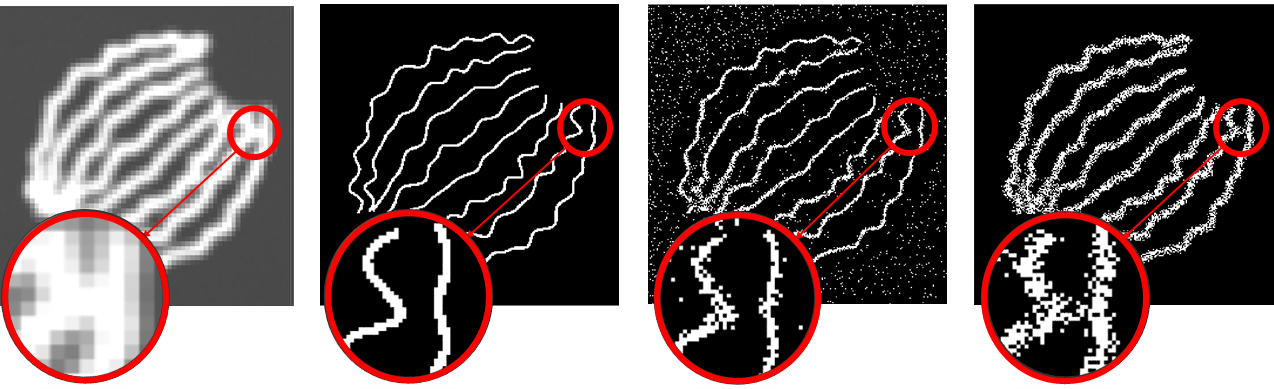
Figure 1: Reconstruction results. From left to right: Observed image, ground truth, $CEL0$ and the proposed algorithm reconstruction.

5 Conclusion

In this paper we have addressed the problem of high-density super-resolution imaging. We have modeled the acquisition system as a $\ell_{2}-\ell_{0}$ constrained problem and proposed a minimizing algorithm. The first numerical results are good but the computational time is quite important due to the minimization of $G_{\rho^{n}}$ for several $\rho^{n}$ and we are working on other approaches for the optimization of the sparse constrained problem.

References

- [1] H. Attouch, J. Bolte, P. Redont, and A. Soubeyran. Proximal alternating minimization and projection methods for nonconvex problems. An approach based on the Kurdyka-Lojasiewicz inequality. arXiv:0801.1780 [math], January 2008. arXiv: 0801.1780.
- [2] A. Beck and M. Teboulle. A Fast Iterative Shrinkage-Thresholding Algorithm for Linear Inverse Problems. SIAM Journal on Imaging Sciences, 2(1):183–202, January 2009.
- [3] E. Betzig, G. H. Patterson, R. Sougrat, O. W. Lindwasser, S. Olenych, J.S. Bonifacino, M. W. Davidson, J. Lippincott-Schwartz, and H. F. Hess. Imaging Intracellular Fluorescent Proteins at Nanometer Resolution. Science, 313(5793):1642–1645, September 2006.
- [4] S. Gazagnes, E. Soubies, and L. Blanc-Féraud. High density molecule localization for super-resolution microscopy using CEL0 based sparse approximation. In 2017 IEEE 14th International Symposium on Biomedical Imaging (ISBI 2017), pages 28–31, April 2017.
- [5] S. T. Hess, T. P. K. Girirajan, and M. D. Mason. Ultra-High Resolution Imaging by Fluorescence Photoactivation Localization Microscopy. Biophysical Journal, 91(11):4258–4272, December 2006.
- [6] M.J. Rust, M. Bates, and X. Zhuang. Sub-diffraction-limit imaging by stochastic optical reconstruction microscopy (STORM). Nature Methods, 3(10):793–796, October 2006.
- [7] D. Sage, H. Kirshner, T. Pengo, N. Stuurman, J. Min, S.uliana Manley, and M. Unser. Quantitative evaluation of software packages for single-molecule localization microscopy. Nature Methods, 12(8):717–724, August 2015.
- [8] E. Soubies, L. Blanc-Féraud, and G. Aubert. A Unified View of Exact Continuous Penalties for l2-l0 Minimization. SIAM Journal on Optimization, 27(3), 2017.
- [9] C. Soussen, J. Idier, D. Brie, and J. Duan. From Bernoulli - Gaussian Deconvolution to Sparse Signal Restoration. IEEE Transactions on Signal Processing, 59(10):4572–4584, October 2011.
- [10] S. M. Stefanov. Convex quadratic minimization subject to a linear constraint and box constraints. Applied Mathematics Research eXpress, 2004(1):17–42, 2004.
- [11] G. Yuan and B. Ghanem. Sparsity Constrained Minimization via Mathematical Programming with Equilibrium Constraints. arXiv preprint arXiv:1608.04430 August 2016.