A Finite Strain Constitutive Model for Martensitic Transformation in Shape Memory Alloys Based on Logarithmic Strain

Abstract

Shape Memory Alloys (SMAs) are materials with the ability to recover apparently permanent deformation under specific thermomechanical loading. The majority of constitutive models for SMAs are developed based on the infinitesimal strain theory. However, such assumption may not be proper in the presence of geometric discontinuities, such as cracks, and repeated cycling loading that has been reported to induce irrecoverable strains up to 20% due to transformation induced plasticity. In addition to finite strains, SMA-based devices may also undergo large rotations. Thus, it is indispensable to develop a constitutive model based on the finite strain to provide accurate predictions of these actuators response. A three-dimensional phenomenological constitutive model for SMAs considering finite strains and finite rotations is proposed in this work. This model utilizes the logarithmic strain as the strain measure that is the strain measure whose logarithmic rate in a corotating material frame is equal to the rate of deformation tensor. In the proposed model, the martensitic volume fraction and the second-order logarithmic transformation strain tensor are chosen as the internal state variables associated with the inelastic transformation process. Numerical simulations considering basic SMAs component geometries such as a bar, a beam, and a torque tube are performed to test the capabilities of the proposed model under both mechanically and thermally induced phase transformation. For numerical examples in which the SMA components exhibits finite strains along with finite rotations, discrepancies are observed between the responses predicted by the present model and its infinitesimal counterpart. Also, the spurious accumulated residual stress observed in infinitesimal strain model is eliminated by the proposed model. This shows that the infinitesimal strain assumption is not applicable in such cases and the proposed model considering large strains and rotations is needed to provide accurate predictions. The presented model formulation will be extended in future work for the incorporation of transformation-induced plasticity.

Nomenclature

$\mathbf{B}$	Left Cauchy-Green tensor
$\mathbf{B}_{i,j}$	Subordinate eigenprojections of $\mathbf{B}$
$\mathbf{D}$	Rate of deformation tensor
$\mathbf{D}^{e}$	Elastic rate of deformation tensor
$\mathbf{D}^{tr}$	Dissipative rate of deformation tensor
$\mathbf{F}$	Deformation gradient
$\mathbf{F}^{e}$	Elastic deformation gradient
$\mathbf{F}^{tr}$	Dissipative deformation gradient
$\mathbf{L}$	Velocity gradient
$\mathbf{S}$	Forth order compliance tensor
$\mathbf{S}^{A}$	Forth order compliance tensor of austenite
$\mathbf{S}^{M}$	Forth order compliance tensor of martensite
$\Delta\mathbf{S}$	Difference of compliance tensor between
	austenite and martensite
$\mathbf{W}$	Anti-symmetric part of velocity gradient
$\mathbf{X}$	Position vector in reference configuration
$\bm{\Lambda}$	Transformation direction tensor
$\bm{\Lambda}^{fwd}$	Forward transformation direction tensor
$\bm{\Lambda}^{rev}$	Reverse transformation direction tensor
$\mathbf{\Omega}^{log}$	Logarithmic spin
$\mathbf{h}$	Logarithmic strain of Eulerian type
$\mathbf{h}^{tr}$	Transformation logarithmic strain
$\mathbf{h}^{tr-r}$	Transformation logarithmic strain at
	reverse point
$\bar{\mathbf{h}}^{tr-r}$	Effective transformation strain at reverse
	point
$\mathbf{x}$	Position vector at current configuration
$\bm{\Upsilon}$	Set of internal state variables
$\bm{\uptau}$	Kirchhoff stress
$\bm{\uptau}^{\prime}$	Deviatoric part of kirchhoff stress
${\bar{\uptau}}^{{}^{\prime}}$	Effective kirchhoff stress
$\bm{\alpha}^{A}$	Second order thermal expansion for austenite
$\bm{\alpha}^{M}$	Second order thermal expansion for martensite
$\Delta\alpha$	Difference of thermal expansion
$\mathcal{D}$	Dissipation energy
$A_{s}$	Austenite transformation start temperature
$A_{f}$	Austenite transformation finish temperature
$M_{s}$	Martensite transformation start temperature
$M_{f}$	Martensite transformation finish temperature
$G$	Gibbs free energy
$H^{max}$	Maximum transformation strain
$T$	Temperature
$T_{0}$	Temperature at reference point
$Y$	Critical thermodynamic driving force
$b_{1},b_{2}$	Material parameters in hardening function
$c$	Specific heat
$\mu_{1},\mu_{2}$	Material parameters in hardening function
$f(\xi)$	Hardening function
$s$	Specific entropy
$s_{0}$	Specific entropy at reference state
$\Delta s_{0}$	Difference of specific entropy
$u$	Internal energy
$u_{0}$	Internal energy at reference state
$\Delta u_{0}$	Difference of internal energy
$\Phi$	Transformation function
$\rho$	Density at current configuration
$\rho_{0}$	Density at reference configuration
$\xi$	Martensite volume fraction
$\nabla$	Gradient operator
$\chi$	Deformation mapping function
$\lambda_{i},\lambda_{j}$	Eigenvalues of $\mathbf{B}$
$\pi$	Thermodynamic driving force

1 Introduction

Shape memory alloys (SMAs) are a kind of specific materials with the ability to recover its pre-defined shape under thermal-mechanical loadings. Since the discovery of shape memory effect phenomenon among metallic alloys from 1930s to 1950s (Otsuka and Wayman, 1932; Greninger and Mooradian, 1938; Kurdjumov and Khandros, 1949; Chang and Read, 1951), shape memory alloys has been extensively investigated to be used as sensors, controllers and actuators etc. towards building smart system integrated with adaptive and intelligent functions.

Over the several past decades, a substantial of SMAs constitutive theories at continuum levels have been proposed, the majority of them are within small deformation regime based on infinitesimal strain assumption. Some thorough review of shape memory models can be found from Boyd and Lagoudas[1], Birman and November[2], Raniecki and Lexcellent [3, 4], Patoor et al.[5, 6], Hackl and Heinen[7], Levitas and Preston [8, 9] etc. In general, these models can be categorized into three different types: crystal-plasticity based model, phase field method based model and phenomenological plasticity based models. In crystal-plasticity based model, it follows the multiplicative decomposition of deformation gradient $\mathbf{F}$ into a recoverable part $\mathbf{F^{e}}$ multiplied by an inelastic dissipative transformation part $\mathbf{F^{tr}}$. One main merit of this model type is it takes into account the crystal orientation, hence it can capture the tension compression asymmetry phenomenon exhibited by many experiment SMAs samples. This kind of model are more physical related from microstructure point of view. However, the complex implementation process of this model type makes it highly computational costly. Some example on crystal-plasticity based models can be found from Auricchio and Taylor[10], Thamburaja and Anand[11], Wang at al.[12], Reese and Christ[13], Yu et al.[14]. Another method to consider microstructure evolution is phase field method based approach. The key point of this method is to utilize an order parameter to differentiate different phases in SMAs, through which it can keep tracking the microstructure changing (like phase boundary) during SMAs transformation process , which makes it particularly suited to studying the dynamic evolution of martensitic microstructures. Some pioneering work related to phase field method can be obtained from Levitas et al.[8, 9], Chen et al.[15], Steinbach et al.[16, 17], Mamivand et al.[18], Zhong and Zhu[19]. On the other hand, phenomenological plasticity based approach is following the legacy of phenomenological $J_{2}$ plasticity theory, it starts from an additive decomposition of total strain into an elastic part plus inelastic or transformation part based on infinitesimal strain assumption, additionally it introduces internal state variables (such as phase volume fraction) to capture the response of bulk material in a macroscopic way. Although it loses microscopic information on microstructure, simplicity of these models and its well established computational implementation procedure makes it widely used in design for SMAs components among engineering field, especially for complex SMAs structure with multiaxial loading conditions. Published and well accepted example models falling into this type can be obtained from literature Lagoudas et al. [20, 21], Brinson et al.[22, 23], Lexcellent et al. [24, 25].

When the deformation regime is within infinitesimal strain range, all the above mentioned models are able to predict material response accurately. However, recent publication has reported that shape memory alloys can reversibly deform to a relatively large strain up to 8% [26, 27], and also repeated cycling loading has been reported to induce irrecoverable transformation induced plasticity strains up to 20% . In addition to such relatively large strains, SMAs-based devices may also undergo finite rotations during its deployment. Combining all the above factors, it is indispensable to develop a constitutive model based on finite deformation framework to provide accurate predictions of these actuators response when deformed. As for the SMA model at the frame work of finite deformation, crystal-plasticity based models utilizing multiplicative decomposition is built within finite-deformation configuration, but again, the implementation complexity of the models hinders its attractiveness for application design. Recent constitutive theories of this model type can be found from literature Auricchio[28], Ziolkowski [29], Christ and Reese[30], Reese and Christ[13], Evangelista et al.[31], Arghavani and Auricchio[32]. On the other hand, phenomenological $J_{2}$ plasticity based models building on infinitesimal strain assumption, though it runs much faster in numerical simulation, may not be proper in the presence of such large strains. Much effort has been devoted to extend this type of model to be used in finite strain deformation analysis. One way is to set up a direct relation between the rate of deformation tensor and an objective rate on a finite strain measure. Utilize the additive decomposition of the rate of deformation tensor $\mathbf{D}$ into an elastic part $\mathbf{D}^{e}$ plus a dissipative part $\mathbf{D}^{tr}$. This approach requires to adopt an objective rate to achieve the principle of objectivity for the rate form hypo-elastic constitutive equation. Well-known existing objective rates such as Zaremba-Jaumann-Noll rate, Green-Naghdi-Dienes rate, Truesdell rate etc. have been proposed to achieve such goal. However, above mentioned objective rates are not real ’objective’, they fail to be integrated from rate form hypo-elastic equation to yield a recoverable hyper-elastic equation. Namely, a non-integrable hypo-elastic formulation is path-dependent and dissipative, and thus would deviate essentially from the recoverable elastic-like behavior[33]. It was not until the logarithmic rate proposed by Xiao et al.[34, 35], Bruhns et al.[36, 37, 38], Meyers et al.[39, 40] that the non-integral issue of objective rates has been resolved.

Moreover, we know a proper finite strain measure is very important for finite deformation analysis. In this paper, we are going to use the logarithmic stain as the finite strain measure, as a result of following reasons: (1)It has been proved by Xiao et al.[34] that the logarithmic rate of logarithmic strain $\mathbf{h}$ is exactly identical with the rate of deformation tensor $\mathbf{D}$, and logarithmic strain is the only one among all other strain measures enjoying this important property, which can be utilized in the thermodynamic framework to make the derivation of constitutive equation in a fully consistent way. (2)Because of the mathematical property of natural logarithm, the total logarithmic strain can be additively decomposed into volumetric part and deviatoric part, while those two portions are inevitably coupled at all other strain measures, such as Green-Lagrange train, used in finite deformation analysis.

Impressed by the above facts, a finite strain constitutive model based on logarithmic strain to analyze the martensitic transformation for shape memory alloys is going to be proposed in this article. The model is based on the SMAs model proposed by Lagoudas and coworkers [1, 20, 21] for small deformation case. To this end, the paper is organized as follows. In Section 2, we represent some preliminaries on kinematics in continuum mechanics. Section 3 will concentrate on the thermodymamics framework to formulate the SMA model by using logarithmic strain and logarithmic rate. Boundary value problems will be addressed to test the capability of proposed model in Section 4. At the end, we summarize this paper with conclusion in Section 5

2 Preliminaries

2.1 Kinematics

Let body $\mathcal{B}$ with its material points defined by position vector $\mathbf{X}$ in the reference (undeformed) configuration at initial time $t_{0}$, and let vector $\mathbf{x}$ represent the position vector occupied by material points $\mathbf{X}$ after deformation at current (deformed) configuration at time $t$, the mapping is defined by $\mathbf{x=\chi}(\mathbf{X},t)$. The deformation process from the initial configuration to current configuration can be characterized by the deformation gradient $\mathbf{F}(\mathbf{x},t)$:

$$\mathbf{F}(\mathbf{x},t)=\frac{\partial\mathbf{x}}{\partial\mathbf{X}}$$ (1)

Then, the velocity gradient $\mathbf{L}$ is defined through as follows:

$$\mathbf{L}=\mathbf{\dot{F}}\mathbf{F}^{-1}$$ (2)

Velocity gradient $\mathbf{L}$ can be additively decomposed into a symmetric part called the rate of deformation tensor, i.e. $\mathbf{D}$, plus an anti-symmetric part called the spin tensor, i.e. $\mathbf{W}$.

$$\begin{array}[]{c}\mathbf{L=D+W};\quad\begin{cases}\mathbf{D}=\dfrac{1}{2}\mathbf{(L+L^{T})},\vspace{5pt}\\ \mathbf{W}=\dfrac{1}{2}\mathbf{(L-L^{T})},\\ \end{cases}\end{array}$$ (3)

The following polar decomposition formula is well known, in which $\mathbf{R}$ is the rotation tensor and $\mathbf{V}$ is the left stretch.

$$\mathbf{F=VR}$$ (4)

The left Cauchy-Green tensor $\mathbf{B}$ is defined by

$$\mathbf{B}=\mathbf{FF}^{T}=\mathbf{V}^{2}$$ (5)

The logarithmic strain of Eulerian type $\mathbf{h}$ is given through,

$$\mathbf{h}=\frac{1}{2}\ln\mathbf{{B}}=\mathbf{\ln{V}}$$ (6)

2.2 Logarithmic rate and Logarithmic spin

In finite elastoplasticity theory, the additive decomposition of the total rate of deformation tensor $\mathbf{D}$ into an elastic part $\mathbf{D}^{e}$ plus a dissipative part $\mathbf{D}^{tr}$ was successfully applied in finite deformation analysis. One of the main job in it is to adopt an appropriate objective rates to achieve the principle of objectivity in rate form equations. Many objective rates have been proposed by different scholars. However, none of them was able to set up a direct relation between the rate of deformation tensor $\mathbf{D}$ and an objective rate of strain measure, thus many spurious phenomenons, such as shear stress oscillation, dissipative energy or residual stress accumulated in elastic deformation etc., are observed. Until recently the so-called logarithmic rate proposed by Xiao et al. [34, 35, 33], Bruhns et al.[36, 37, 38], Meyers et al.[39, 40] successfully resolved such self-inconsistent issues. As they showed that the logarithmic rate of the logarithmic strain $\mathbf{h}$ of Eulerian type is identical with the rate of deformation tensor $\mathbf{D}$, which is expressed as:

$$\mathring{\mathbf{h}}^{log}=\dot{\mathbf{h}}+\mathbf{h}\mathbf{\Omega}^{log}-\mathbf{\Omega}^{log}\mathbf{h}=\mathbf{D}$$ (7)

Where $\mathring{\mathbf{h}}^{log}$ means the logarithmic rate of logarithmic strain and $\dot{\mathbf{h}}$ is the conventional time rate of logarithmic strain. $\mathbf{\Omega}^{log}$ is called logarithmic spin introduced by Xiao and Bruhns [34] with explicit expression as:

$$\mathbf{\Omega}^{log}=\mathbf{W}+\sum_{i\neq j}^{n}\big{(}\frac{1+(\lambda_{i}/\lambda_{j})}{1-(\lambda_{i}/\lambda_{j})}+\frac{2}{\textbullet\ln(\lambda_{i}/\lambda_{j})}\big{)}\mathbf{B}_{i}\mathbf{D}\mathbf{B}_{j}$$ (8)

Where $\mathbf{W}$ is the spin tensor; $\lambda_{i,j}(i,j=1,2,3...)$ are the eigenvalues of Left Cauchy-Green tensors $\mathbf{B}$; $\mathbf{B}_{i,j}$ are the corresponding subordinate eigenprojections of $\mathbf{B}$. Equation 7 is very important in consistent formulation of finite strain SMAs model at following thermodynamic framework later on .

2.3 Additive decomposition of logarithmic strain

Starting from additive decomposition of $\mathbf{D}$ in kinematics for deformation,

$$\mathbf{D}=\mathbf{D}^{e}+\mathbf{D}^{tr}$$ (9)

The total stress power supplied from outside working on body $\mathcal{B}$ per unit volume can be calculated and additively decomposed into,

$$P_{stress\_power}=\bm{\uptau}:\mathbf{D}=\bm{\uptau}:\mathbf{D}^{e}+\bm{\uptau}:\mathbf{D}^{tr}$$ (10)

From energy point of view, additive decomposition in deformation kinematics can be interpreted as total stress power being split into a recoverable part as $\bm{\uptau}:\mathbf{D}^{e}$ plus an irrecoverable part as $\bm{\uptau}:\mathbf{D}^{tr}$ associated with dissipative process (such as plasticity deformation, transformation process etc.).

By virtue of equation 7, elastic part $\mathbf{D}^{e}$ and dissipative part $\mathbf{D}^{tr}$ in equation 9 can be rewritten as the logarithmic rate of elastic logarithmic strain ${\mathbf{h}}^{e}$ and the logarithmic rate of transformation logarithmic strain ${\mathbf{h}}^{tr}$ respectively,

$$\mathring{\mathbf{h}}^{e\_log}=\mathbf{D}^{e};~{}~{}\mathring{\mathbf{h}}^{tr\_log}=\mathbf{D}^{tr}$$ (11)

Combine equation 9 and equation 11, the following equation can be obtained.

$$\mathring{\mathbf{h}}^{log}=\mathring{\mathbf{h}}^{e\_log}+\mathring{\mathbf{h}}^{tr\_log}$$ (12)

Apply logarithmic corotational integration[41] in equation 12 on both sides, the following additive decomposition of total logarithmic strain can be received. Namely, the total logarithmic strain can be additively split into an elastic part corresponding to recoverable energy and transformation part associated with dissipated energy in transformation process.

$$\mathbf{h}=\mathbf{h}^{e}+\mathbf{h}^{tr}$$ (13)

3 Model Formulation

3.1 General thermodynamic framework

In order to develop finite strain SMAs model, we start with definition of the Gibbs free energy $G$ to be a continuous function dependent on Kirchhoff stress tensor $\bm{\uptau}$, logarithmic strain of Eulerian type $\mathbf{h}$, temperature $T$, specific entropy $s$, and a set of internal state variables $\bm{\Upsilon}$ to be confirmed later on.

$$G(\bm{\uptau},\mathbf{h},T,s,\bm{\Upsilon})=u-\dfrac{1}{\rho_{0}}\bm{\uptau}:\mathbf{h}-sT$$ (14)

$G$ is the Gibbs free energy, $\rho_{0}$ is the density at reference configuration, $s$ is specific entropy and $u$ is internal energy. Later on, logarithmic transformation strain $\mathbf{h}^{tr}$ and the martensitic volume fraction $\xi$ will be chosen as internal state variables to model the SMAs nonlinear material response.

Based on the $2^{nd}$ law of thermodynamics, the dissipation energy $\mathcal{D}$ can be written in the form of Clausius-Duhem inequality,

$$\mathcal{D}=\mathbf{\bm{\sigma}:D}-\rho(\dot{u}-T\dot{s})\geqslant 0$$ (15)

$\rho$ is density at current configuration. Since Gibbs free energy is a continuous function as defined in equation 14, take the logarithmic rate of equation 14. Considering objective rates on a scalar variable equals to conventional time rate of that scalar, we are able to derive equation 16. From now on, the log symbol in logarithmic rate will be ignored in later part for text legibility.

$$\mathring{G}^{log}=\dot{G}=\dot{u}-\dfrac{1}{\rho_{0}}\mathring{\bm{\uptau}}^{log}:\mathbf{h}-\dfrac{1}{\rho_{0}}\bm{\uptau}:\mathring{\mathbf{h}}^{log}-s\dot{T}-\dot{s}T$$ (16)

After some math on 16, we end up with equation 17 of the Gibbs free energy.

$$\dot{u}-\dot{s}T=\dot{G}+\dfrac{1}{\rho_{0}}\mathring{\bm{\uptau}}:\mathbf{h}+\dfrac{1}{\rho_{0}}\bm{\uptau}:\mathring{\mathbf{h}}+s\dot{T}$$ (17)

Substitute equation 17 into equation 15, the dissipation energy can be reformulated as follows,

$$\mathcal{D}=-\rho_{0}\dot{G}-\rho_{0}s\dot{T}-\mathring{\bm{\uptau}}:\mathbf{h}\geqslant 0$$ (18)

Again, invoking Gibbs free energy is continuous, we are allowed to take chain rule differentiation on $G$ with respect to its independent variables. Noted $\bm{\uptau}$ and $\mathbf{h}$ are conjugate pair, and $s$ is also conjugated to $T$, only one from each of them is independent variable of Gibbs free energy $G$.

$$\dot{G}=\mathring{G}^{log}=\frac{\partial G}{\partial\bm{\uptau}}:\mathring{\bm{\uptau}}+\frac{\partial G}{\partial T}\dot{T}+\frac{\partial G}{\partial\bm{\Upsilon}}:\mathring{\bm{\Upsilon}}$$ (19)

Substitute equation 19 into equation 18, following equation for the dissipation energy $\mathcal{D}$ is derived :

$$\mathcal{D}=-(\rho_{0}\frac{\partial G}{\partial\bm{\uptau}}+\mathbf{h}):\mathring{\bm{\uptau}}-(\rho_{0}\frac{\partial G}{\partial T}+s):\dot{T}-\rho_{0}\frac{\partial G}{\partial\bm{\Upsilon}}:\mathring{\bm{\Upsilon}}\geqslant 0$$ (20)

Follow standard Coleman-Noll procedure, no matter what the thermodynamic path the system will have, the dissipation energy $\mathcal{D}$ should always be greater than zero in order to satisfy the $2^{nd}$ thermodynamics law. the following constitutive relationship between conjugate pairs will be obtained.

$$s=-\rho_{0}\frac{\partial G}{\partial T}$$ (21)

$$\mathbf{h}=-\rho_{0}\frac{\partial G}{\partial\bm{\uptau}}$$ (22)

Apply constitutive equation 21 and equation 22 into dissipation energy inequality 20, we have the following strict from of dissipation inequality.

$$-\rho_{0}\frac{\partial G}{\partial\bm{\Upsilon}}:\mathring{\bm{\Upsilon}}\geqslant 0$$ (23)

3.2 Constitutive modeling for SMAs at finite strain

3.2.1 Thermodynamic potential of constitutive model

In this section, the general thermodynamic framework derived previously will be used to formulate the finite strain constitutive modeling for SMAs. This work is based on the infinitesimal strain model proposed by Lagoudas and coworkers [1, 20, 21], which has been extensively used for the design and development of SMA-based active device and smart structures [42, 43, 44] for the past two decades. We begin with an explicit expression for Gibbs free energy for start point. Independent variables of Gibbs free energy $G$ are chosen as kirchhoff stress $\bm{\uptau}$ and temperature $T$. Transformation logarithmic strain $\mathbf{h}^{tr}$ and martensitic volume fraction $\xi$ are chosen as a set of internal state variables $\mathbf{\Upsilon}=\{\mathbf{h}^{tr},\xi\}$ to model the SMAs nonlinear material response. Transformation logarithmic strain $\mathbf{h}^{tr}$ is accounting for the inelastic strain part caused by transformation between austenite and martensite phase, the martensite volume fraction $\xi$ ranging from $0$ to $1$ is used for differentiating the two different phases in SMAs, the explicit Gibbs free energy is given as:

$$G(\bm{\uptau},T,\mathbf{h}^{tr},\xi)=-\dfrac{1}{2\rho_{0}}\bm{\uptau}:\mathbf{S}:\bm{\uptau}-\dfrac{1}{\rho_{0}}\bm{\uptau}:[~{}\bm{\alpha}(T-T_{0})+\mathbf{h}^{tr}]$$ (24)

$$+c\Big{[}(T-T_{0})-T\ln(\dfrac{T}{T_{0}})\Big{]}-s_{0}T+u_{0}+\dfrac{1}{\rho_{0}}f(\xi)$$

$\mathbf{S}$ is the fourth-order compliance tensor dependent on martensitic volume fraction $\xi$, it is calculated by using a rule of mixtures as defined by equation 25, $\bm{\alpha}$ is the second order thermoelastic expansion tensor, $\mathbf{h}^{tr}$ is transformation logarithmic strain, $c$ is effective specific heat, $s_{0},u_{0}$ are effective specific entropy at reference state and effective specific internal energy at reference state, respectively, they are defined similar as equation 25 by virtue of rule of mixtures; $T$ denotes current temperature while $T_{0}$ is reference temperature. $f(\xi)$ is a transformation hardening function upon being defined later on.

$$\mathbf{S}(\xi)=\mathbf{S}^{A}+\xi(\mathbf{S}^{M}-\mathbf{S}^{A})=\mathbf{S}^{A}+\xi\Delta\mathbf{S}$$ (25)

Using rule of mixture to calculate the effective compliance tensor in equation 25, $\mathbf{S}^{A}$ is forth order compliance tensor for austenite phase, $\mathbf{S}^{B}$ is forth order compliance tensor for martensite phase, and $\Delta\mathbf{S}$ is the difference between them.

From Lagoudas infinitesimal model[1, 20, 21], we take the same hardening function as defined by equation 26, in which $b^{A},b^{M},\mu_{1},\mu_{2}$ are material parameters defined in equation 36.

$$f(\xi)=\begin{cases}\dfrac{1}{2}\rho_{0}b^{M}{\xi}^{2}+(\mu_{1}+\mu_{2})\xi,\;\dot{\xi}>0,\vspace{5pt}\\ \dfrac{1}{2}\rho_{0}b^{A}{\xi}^{2}+(\mu_{1}-\mu_{2})\xi,\;\dot{\xi}<0,\end{cases}\\$$ (26)

To this end, Gibbs free energy $G$ is explicitly defined in equation 24. The next step is to apply it to general thermodynamic framework to obtain constitutive equations. Substitute Gibbs free energy expression into equation 21 to obtain the constitutive relation for entropy $s$, and also substitute into equation 22 to obtain the constitutive relation for logarithmic strain $\mathbf{h}$.

$$s=-\rho_{0}\frac{\partial G}{\partial T}=\dfrac{1}{\rho_{0}}\bm{\uptau}:\bm{\alpha}+c\ln(\dfrac{T}{T_{0}})+s_{0}$$ (27)

$$\mathbf{h}=-\rho_{0}\frac{\partial G}{\partial\bm{\uptau}}=\mathbf{S~{}\bm{\uptau}}+\bm{\alpha}(T-T_{0})+\mathbf{h}^{tr}$$ (28)

Transformation logarithmic strain $\mathbf{h}^{tr}$ and martensite volume fraction $\xi$ are internal state variables to model the nonlinear system. Rewrite the strict from dissipation inequality equation (23) by choosing the set of internal state variables $\mathbf{\Upsilon}=\{\mathbf{h}^{tr},\xi\}$

$$-\rho_{0}\frac{\partial G}{\partial\mathbf{h}^{tr}}:\mathring{\mathbf{h}}^{tr}-\rho_{0}\frac{\partial G}{\partial\xi}\dot{\xi}\geqslant 0$$ (29)

3.2.2 Evolution equation of internal state variables

In the subsection, we will set up the evolution equation between transformation logarithmic strain $\mathbf{h}^{tr}$ and martensite volume fraction $\xi$. In this model, only detwinned martensite variant is considered in the transformation process. One key assumption from Lagoudas infinitesimal model is: any change in the current microstructural state of the material is strictly a result of a change in the martensitic volume fraction (Boyd and Lagoudas[1, 20]). The rigorous mathematical derivation of this assumption is provided by Qidwai and Lagoudas [45], in which they used the principle of maximum dissipation and the $J_{2}$ plasticity theory to derive that the remaining internal state variables in strict form of dissipation inequality 29 is directly proportional to the evolution of martensitic volume fraction $\xi$. Inspired from that, we thus propose the following evolution relationship between $\mathbf{h}^{tr}$ and $\xi$.

$${\mathring{\mathbf{h}}}^{tr}=\bm{\Lambda}\dot{\xi},\ \ \bm{\Lambda}=\begin{cases}\bm{\Lambda}^{fwd},\;\dot{\xi}>0,\vspace{5pt}\\ \bm{\Lambda}^{rev},\;\dot{\xi}<0,\end{cases}\\$$ (30)

where, $\bm{\Lambda}^{fwd}$ is the transformation direction tensor during forward transformation process, while $\bm{\Lambda}^{rec}$ is the transformation direction tensor during reverse transformation process , they are defined as following:

$$\bm{\Lambda}^{fwd}=\frac{3}{2}H^{max}\frac{\bm{\uptau}^{{}^{\prime}}}{\bar{\uptau}^{{}^{\prime}}},\ \bm{\Lambda}^{rev}=H^{max}\frac{\mathbf{h}^{tr-r}}{{\xi}^{r}}.$$ (31)

In which, $H^{max}$ is a material parameter denoting the maximum transformation strain. In forward transformation direction tensor, $\bm{\uptau}^{{}^{\prime}}$ is the deviatoric stress tensor calculated by $\bm{\uptau}^{{}^{\prime}}=\bm{\uptau}-{\small\frac{1}{3}}\textrm{tr}(\bm{\uptau})~{}\mathbf{I}$, where $\mathbf{I}$ is the second order identity tensor. The effective (von Mises equivalent) stress is given by $\bar{\uptau}^{{}^{\prime}}={\small\sqrt{{{\small\frac{3}{2}}\bm{\uptau}}^{{}^{\prime}}:\bm{\uptau}^{{}^{\prime}}}}$. In reverse transformation direction tensor, $\mathbf{h}^{tr-r}$ represents the transformation logarithmic strain at the reverse transformation starting point; ${\xi}^{r}$ denotes the martensitic volume fraction at the reverse transformation starting point. The definition of transformation tensor is based on the assumption that transformation strain will evolve following the direction of deviatoric stress during forward $(\dot{\xi}>0)$. During the reverse transformation $(\dot{\xi}<0)$, the transformation strain will decrease proportionally from the value at reversal starting point to the finish value of reverse transformation.

3.2.3 Transformation function

After define the evolution equation between the transformation logarithmic strain $\mathbf{h}^{tr}$ and the martensitic volume fraction $\xi$ in section 3.2.2, the next objective is to define a proper transformation function as criteria to determine when the transformation will happen. Substitute the evolution equation 30 into the dissipation inequality (29), we obtain the following equation:

$$(\bm{\uptau}:\bm{\Lambda}-\rho_{0}\frac{\partial G}{\partial\xi})\dot{\xi}=\pi\dot{\xi}\geqslant 0$$ (32)

Where, the scalar quantity $\pi$ is called general thermodynamic driving force conjugated to $\xi$. Substitute the specific Gibbs free energy expression equation 24 into equation 32, the expression for general thermodynamic driving force $\pi$ is given by:

$$\pi(\bm{\uptau},T,\xi)=\bm{\uptau}:\bm{\Lambda}+\dfrac{1}{2}\bm{\uptau}:{\Delta}\mathbf{S}:\bm{\uptau}+\bm{\uptau}:{\Delta}\mathbf{\alpha}(T-T_{0})-\rho_{0}\Delta c$$ (33)

$$\big{[}T-T_{0}-T\ln(\dfrac{T}{T_{0}})\big{]}+\rho_{0}\Delta s_{0}T-\rho_{0}\Delta u_{0}-\frac{\partial f}{\partial\xi}$$

Where, material parameters $\Delta\mathbf{\alpha},\Delta c,\Delta s_{0},\Delta u_{0}$ represents the difference for different phases. They have similar definition as $\Delta\mathbf{S}$ in equation (25). From Lagoudas model, we are also assuming that whenever the thermodynamic driving force $\pi$ reach a critical value $Y$ (or $-Y$), the forward (reverse) phase transformation will take place. Thus we introduce a transformation function $\Phi$ defined by (34) as the criteria to determine whether forward and reverse transformation happens.

$${\Phi}=\begin{cases}~{}~{}\pi-Y,\;\dot{\xi}>0,\vspace{5pt}\\ -\pi-Y,\;\dot{\xi}<0,\end{cases}\\$$ (34)

It is proved from Qidwai and Lagoudas[45] that some certain constraints have to be applied on the evolution of martensitic volume fraction $\xi$, this constraint can be expressed as so-called Kuhn-Tucker conditions:

$$\dot{\xi}\geqslant 0;\quad\Phi(\bm{\uptau},T,\xi)=~{}~{}\pi-Y\leqslant 0;\quad\Phi\dot{\xi}=0;~{}~{}~{}\bf{(A\Rightarrow M)}$$ (35)

$$\dot{\xi}\leqslant 0;\quad\Phi(\bm{\uptau},T,\xi)=-\pi-Y\leqslant 0;\quad\Phi\dot{\xi}=0;~{}~{}~{}\bf{(M\Rightarrow A)}$$

The critical value $Y$ together with the other material parameters $(b^{A},b^{M},\mu_{1},\mu_{2})$ defined in the hardening function (26) are determined from the phase diagram parameters $(M_{s},M_{f},A_{s},A_{f},\Delta s_{0},\Delta u_{0})$. The readers themselves are encouraged to find calibration details through the book authored by Lagoudas and coworskers [20].

$$\begin{cases}Y=\tfrac{1}{4}\rho_{0}\Delta s_{0}(M_{s}+M_{f}-A_{s}-A_{f})\\ b^{A}=-\Delta s_{0}(A_{f}-A_{s})\\ b^{M}=-\Delta s_{0}(M_{s}-M_{f})\\ \mu_{1}=\tfrac{1}{2}\rho_{0}\Delta s_{0}(M_{s}+M_{f})-\rho_{0}\Delta u_{0}\\ \mu_{2}=\tfrac{1}{4}\rho_{0}\Delta s_{0}(A_{s}-A_{f}-M_{f}+M_{s})\end{cases}$$ (36)

4 Numerical Results

In this section, several boundary value problems, such as a simple SMAs bar under actuation loading, a SMAs beam under bending loading, and a SMAs tube under torsion loading are gonging to be analyzed to test the capability of the proposed finite strain SMAs model. The results, such as actuation loading curve and accumulated residual stress, predicted by proposed finite strain model and its infinitesimal counterpart will be compared.

4.1 Bar Actuation Problem

The first boundary value problem analyzed is a simple SMAs bar under actuation loading. The bar length is $L=100$ mm, the cross section is a square with its edge length $a=10$mm.The boundary conditions are left face fixed in all degrees of freedom and the right face subject to constant pressure.

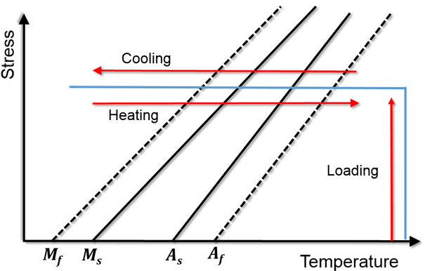
Figure 1: Loading path for bar actuation problem

As depicted in loading diagram 1, the bar is first loaded up to constant pressure 30 MPa. Then, the bar is cool down from the initial temperature 360^∘C to lower temperature 220^∘C. The SMA bar will experience a large extension due to its forward transformation from austenite phase to detwinned martensite phase. The next step is increasing temperature from 220^∘C to 360^∘C, the bar will contract to its original length due to the reverse transformation from detwinned martensite phase to austenite phase. This SMAs bar experienced a full actuation loading cycle. The material parameters utilized in this SMAs bar analysis is from table 1[20].

Table 1: Material parameters of SMAs

	EA	EM	Ms	Mf	As	Af
	90 GPa	47 GPa	308∘C	246∘C	284∘C	356∘C
	$\alpha_{A}$	$\alpha_{M}$	$\textit{v}_{A}$	$\textit{v}_{M}$
	2.2e-5	2.2e-5	0.33	0.33

In this simple SMAs bar actuation problem, the results predicted from both proposed finite strain and infinitesimal strain model are compared in figure 2, which are plotted by temperature versus displacement. As the results showing in figure 2, with the material parameter maximum transformation strain ${H}^{max}=10\%$, the predicted results between the infinitesimal model and the proposed finite strain model is slightly different.

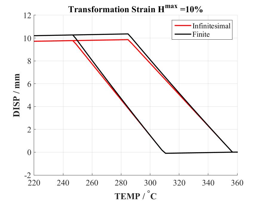
Figure 2: ${H}^{max}=10\%$

4.2 Beam Bending Problem

The second problem analyzed is a three dimensional SMA beam under bending. The material parameters used are also from table 1. Boundary conditions are left side fixed in all degrees of freedom and the right side free to move at all directions. The loading path is described as figure 3. The beam starts from austenite phase under bending pressure which is gradually increasing from zero to maximum value. The SMAs beam undergoes a forward stress-induced phase transformation from austnite phase to detwinned martensite phase. Then, the pressure gradually decreases from maximum to zero, during which the beam experiences a reverse transformation from detwinned martensite phase to austenite phase.

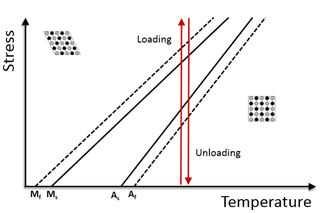
Figure 3: Loading path for beam bending problem

During this loading cycle, phase transformation in SMAs is the only fact accounting for inelastic material response. So once it is fully recovered from the transformation, the SMAs beam should be able to return to unstress state. However, different numerical results are observed between finite strain SMAs model and its infinitesimal counterpart.

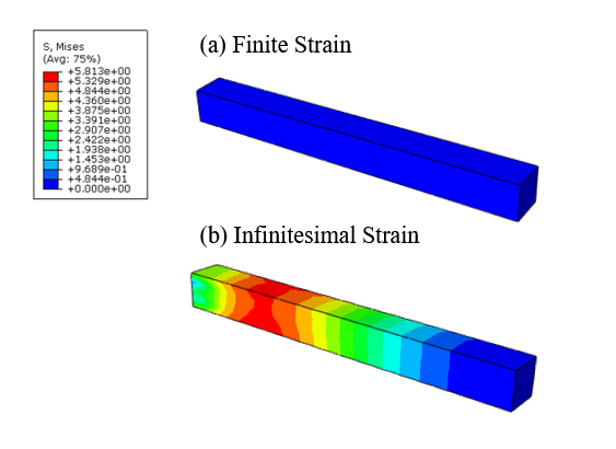
Figure 4: Accumulated residual von mises stress of beam after bending

As irt shows in figure 4(a), residual von mises stress results given by finite strain SMAs model has magnitude of $10^{-5}$ in the end. As a comparison, residual von mises stress results predicted by infinitesimal strain model is around a nontrivial 5 MPa at the end of the loading. This comparison shows for SMAs components with large rotations, response predicted by infinitesimal strain model will accumulate spurious residual stress at the end of the loading, while this can be eliminated by using a proposed finite strain model. This demonstrates a consistent finite strain model is needed to provide more accurate results.

4.3 Torque Tube Problem

Boundary value problem of hollow cylindrical torque tube under torsion loading is solved in this section. In this problem, apart from the large shear strain SMAs will exhibit, it also undertakes large geometry rotations. The boundary conditions are described in figure 5, The tube left face is fixed in all degrees of freedom and tube right face is subject to twist $\theta_{z}(t)$ angle along z axis. The material parameters are also choosing from table 1, the maximum transformation strain is ${H}^{max}=5\%$ in this case.

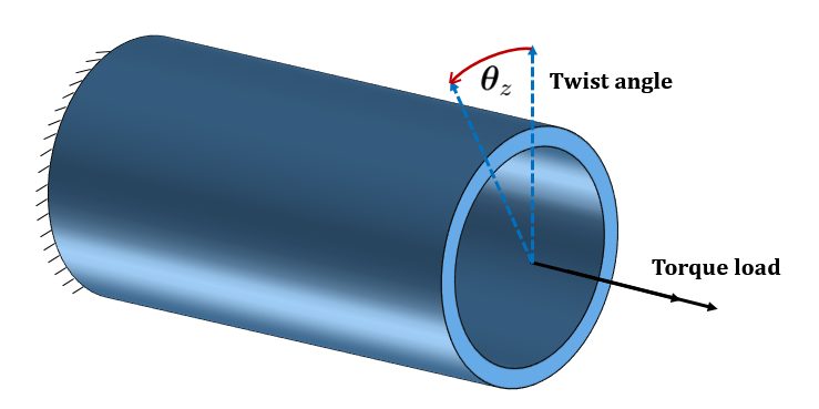
Figure 5: Schematic for torque tube problem

The loading history for troque tube is in figure 6. The tube starts with zero twist angle in austenite phase. Then, the twist angle is gradually increasing proportionally from zero to a maximum value. After twist angle reaches the peak amplitude, it gradually decreases linearly from peak to the zero value at the end of loading. The SMAs tube will experience a full pseudoelastic loading cycle.

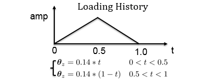
Figure 6: Torque tube loading history

Difference on predicted results are observed on accumulated residual stress at the end of loading cycle. Since transformation is the only inelastic process considered in SMAs for current analysis, torque tube should return to unstressed state once it fully recover from the torsion loading. As showed on the left picture in figure 7, this was correctly simulated by the proposed finite strain model. However, it is not the case for the results received from infinitesimal strain model. The residual stress remain around 4 MPa at the end of loading as showing in right picture of figure 7. It is discussed in the introduction part, the residual stress is coming from the non-integral issue of many objective rates have. As spurious residual stress accumulated through a number of loading cycles, it may even triggers the transformation to happen which should not be the real case in reality. Using the consistent finite strain model based on logarithmic strain and logarithmic rate will resolve this problem. Again, the residual stress results in torque tube problem demonstrate the necessity of utilizing the proposed finite strain model to predict the SMAs response under large deformations.

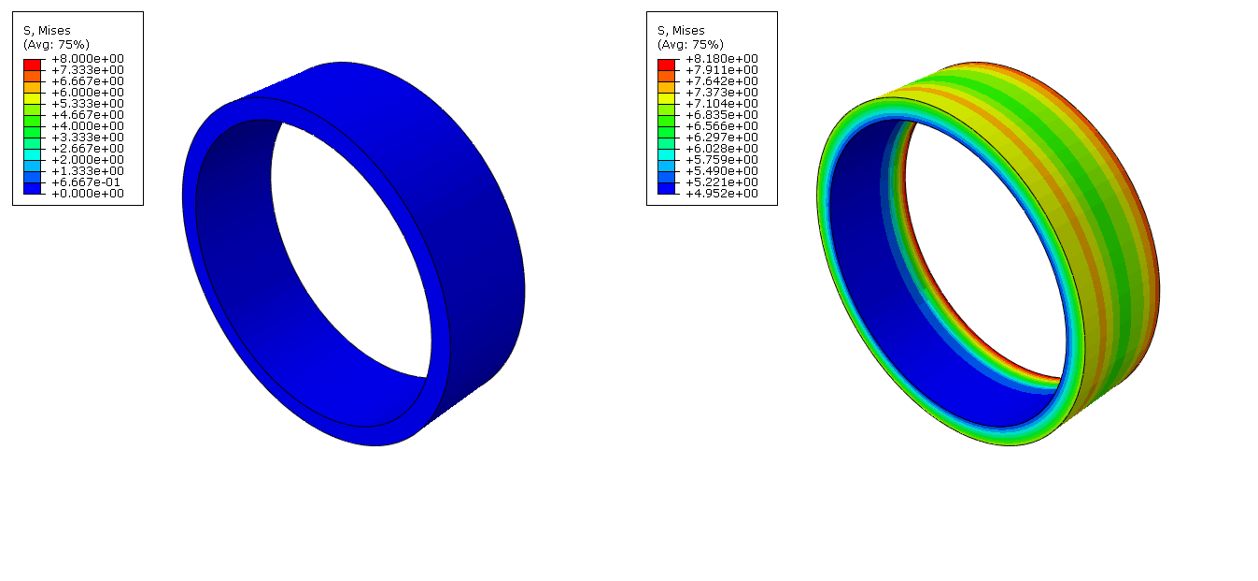
Figure 7: Accumulated residual von mises stress for torque tube after torsion

5 Conclusions

Based on the constitutive model for shape memory alloys within small deformation range proposed by Lagoudas and coworkers[boyd1998, 20, 21], a three dimensional constitutive model for martensitic transformation in shape memory alloys is formulated based on additive decomposition of the rate of deformation tensor. The model is derived fully consistently within thermodynamic framework by utilizing the logarithmic strain as finite strain measure, whose logarithmic rate is equivalent to the rate of deformation tensor. The martensitic volume fraction and the second-order transformation logarithmic strain tensor are chosen as the internal state variables accounting for the inelastic transformation process. Numerical simulations considering basic SMA component geometries such as a bar, a beam and a torque tube are performed to test the capabilities of proposed model under both mechanically and thermally induced phase transformation. For numerical examples in simple bar with maximum transformation strain ${H^{max}=10\%}$, discrepancies are observed between the responses predicted by the proposed model and its infinitesimal counterpart. Also, spurious residual stress observed in predicted results by infinitesimal strain model are successfully eliminated by proposed model. This shows that the infinitesimal strain assumption is not applicable when SMA components exhibit finite strains along with finite rotations, the proposed consistent finite strain model based on logarithmic strain and logarithmic rate is needed to give more accurate results. The presented formulation will be extended in future work for considering transformation-induced plasticity in cyclic loadings.

6 Acknowledgments

The author is deeply grateful for the financial support provided by the Qatar National Research Fund under Grant NPRP 7-032-2-016.

References

- [1] Boyd, J. G. and Lagoudas, D. C., “A thermodynamical constitutive model for shape memory materials. Part I. The monolithic shape memory alloy,” International Journal of Plasticity, Vol. 12, No. 6, 1996, pp. 805–842.
- [2] Birman, V., “Review of mechanics of shape memory alloy structures,” Applied Mechanics Reviews, Vol. 50, No. 11, 1997, pp. 629–645.
- [3] Raniecki, B., Lexcellent, C., and Tanaka, K., “Thermodynamic models of pseudoelastic behaviour of shape memory alloys,” Archiv of Mechanics, Archiwum Mechaniki Stosowanej, Vol. 44, 1992, pp. 261–284.
- [4] Raniecki, B. and Lexcellent, C., “Thermodynamics of isotropic pseudoelasticity in shape memory alloys,” European Journal of Mechanics-A/Solids, Vol. 17, No. 2, 1998, pp. 185–205.
- [5] Patoor, E., Lagoudas, D. C., Entchev, P. B., Brinson, L. C., and Gao, X., “Shape memory alloys, Part I: General properties and modeling of single crystals,” Mechanics of materials, Vol. 38, No. 5, 2006, pp. 391–429.
- [6] Patoor, E., Eberhardt, A., and Berveiller, M., “Micromechanical modelling of superelasticity in shape memory alloys,” Le Journal de Physique IV, Vol. 6, No. C1, 1996, pp. C1–277.
- [7] Hackl, K. and Heinen, R., “A micromechanical model for pretextured polycrystalline shape-memory alloys including elastic anisotropy,” Continuum Mechanics and Thermodynamics, Vol. 19, No. 8, 2008, pp. 499–510.
- [8] Levitas, V. I., “Thermomechanical theory of martensitic phase transformations in inelastic materials,” International Journal of Solids and Structures, Vol. 35, No. 9, 1998, pp. 889–940.
- [9] Levitas, V. I. and Preston, D. L., “Three-dimensional Landau theory for multivariant stress-induced martensitic phase transformations. I. Austenite-martensite,” Physical review B, Vol. 66, No. 13, 2002, pp. 134206.
- [10] Auricchio, F. and Taylor, R. L., “Shape-memory alloys: modelling and numerical simulations of the finite-strain superelastic behavior,” Computer methods in applied mechanics and engineering, Vol. 143, No. 1, 1997, pp. 175–194.
- [11] Thamburaja, P. and Anand, L., “Polycrystalline shape-memory materials: effect of crystallographic texture,” Journal of the Mechanics and Physics of Solids, Vol. 49, No. 4, 2001, pp. 709–737.
- [12] Wang, X., Xu, B., and Yue, Z., “Micromechanical modelling of the effect of plastic deformation on the mechanical behaviour in pseudoelastic shape memory alloys,” International Journal of Plasticity, Vol. 24, No. 8, 2008, pp. 1307 – 1332.
- [13] Reese, S. and Christ, D., “Finite deformation pseudo-elasticity of shape memory alloys–constitutive modelling and finite element implementation,” International Journal of Plasticity, Vol. 24, No. 3, 2008, pp. 455–482.
- [14] Yu, C., Kang, G., Kan, Q., and Song, D., “A micromechanical constitutive model based on crystal plasticity for thermo-mechanical cyclic deformation of NiTi shape memory alloys,” International Journal of Plasticity, Vol. 44, 2013, pp. 161–191.
- [15] Chen, L.-Q., “Phase-field models for microstructure evolution,” Annual review of materials research, Vol. 32, No. 1, 2002, pp. 113–140.
- [16] Steinbach, I. and Pezzolla, F., “A generalized field method for multiphase transformations using interface fields,” Physica D: Nonlinear Phenomena, Vol. 134, No. 4, 1999, pp. 385–393.
- [17] Steinbach, I. and Apel, M., “Multi phase field model for solid state transformation with elastic strain,” Physica D: Nonlinear Phenomena, Vol. 217, No. 2, 2006, pp. 153–160.
- [18] Mamivand, M., Zaeem, M. A., and El Kadiri, H., “A review on phase field modeling of martensitic phase transformation,” Computational Materials Science, Vol. 77, 2013, pp. 304–311.
- [19] Zhong, Y. and Zhu, T., “Phase-field modeling of martensitic microstructure in NiTi shape memory alloys,” Acta Materialia, Vol. 75, 2014, pp. 337–347.
- [20] Lagoudas, D. C., “Shape memory alloys,” Science and Business Media, LLC, 2008.
- [21] Lagoudas, D., Hartl, D., Chemisky, Y., Machado, L., and Popov, P., “Constitutive model for the numerical analysis of phase transformation in polycrystalline shape memory alloys,” International Journal of Plasticity, Vol. 32, 2012, pp. 155–183.
- [22] Brinson, L. and Lammering, R., “Finite element analysis of the behavior of shape memory alloys and their applications,” International Journal of Solids and Structures, Vol. 30, No. 23, 1993, pp. 3261–3280.
- [23] Brinson, L. C., “One-dimensional constitutive behavior of shape memory alloys: thermomechanical derivation with non-constant material functions and redefined martensite internal variable,” Journal of intelligent material systems and structures, Vol. 4, No. 2, 1993, pp. 229–242.
- [24] Leclercq, S. and Lexcellent, C., “A general macroscopic description of the thermomechanical behavior of shape memory alloys,” Journal of the Mechanics and Physics of Solids, Vol. 44, No. 6, 1996, pp. 953–980.
- [25] Lexcellent, C., Shape-memory alloys handbook, John Wiley & Sons, 2013.
- [26] Jani, J. M., Leary, M., Subic, A., and Gibson, M. A., “A review of shape memory alloy research, applications and opportunities,” Materials & Design, Vol. 56, 2014, pp. 1078–1113.
- [27] Shaw, J. A., “Simulations of localized thermo-mechanical behavior in a NiTi shape memory alloy,” International Journal of Plasticity, Vol. 16, No. 5, 2000, pp. 541–562.
- [28] Auricchio, F., “A robust integration-algorithm for a finite-strain shape-memory-alloy superelastic model,” International Journal of plasticity, Vol. 17, No. 7, 2001, pp. 971–990.
- [29] Ziolkowski, A., “Three-dimensional phenomenological thermodynamic model of pseudoelasticity of shape memory alloys at finite strains,” Continuum Mechanics and Thermodynamics, Vol. 19, No. 6, 2007, pp. 379–398.
- [30] Christ, D. and Reese, S., “A finite element model for shape memory alloys considering thermomechanical couplings at large strains,” International Journal of solids and Structures, Vol. 46, No. 20, 2009, pp. 3694–3709.
- [31] Evangelista, V., Marfia, S., and Sacco, E., “A 3D SMA constitutive model in the framework of finite strain,” International Journal for Numerical Methods in Engineering, Vol. 81, No. 6, 2010, pp. 761–785.
- [32] Arghavani, J., Auricchio, F., and Naghdabadi, R., “A finite strain kinematic hardening constitutive model based on Hencky strain: general framework, solution algorithm and application to shape memory alloys,” International Journal of Plasticity, Vol. 27, No. 6, 2011, pp. 940–961.
- [33] Xiao, H., Bruhns, O., and Meyers, A., “Elastoplasticity beyond small deformations,” Acta Mechanica, Vol. 182, No. 1-2, 2006, pp. 31–111.
- [34] Xiao, H., Bruhns, I. O., and Meyers, I. A., “Logarithmic strain, logarithmic spin and logarithmic rate,” Acta Mechanica, Vol. 124, No. 1-4, 1997, pp. 89–105.
- [35] Xiao, H., Bruhns, O., and Meyers, A., “Hypo-elasticity model based upon the logarithmic stress rate,” Journal of Elasticity, Vol. 47, No. 1, 1997, pp. 51–68.
- [36] Bruhns, O., Xiao, H., and Meyers, A., “Self-consistent Eulerian rate type elasto-plasticity models based upon the logarithmic stress rate,” International Journal of Plasticity, Vol. 15, No. 5, 1999, pp. 479–520.
- [37] Bruhns, O., Xiao, H., and Meyers, A., “Large simple shear and torsion problems in kinematic hardening elasto-plasticity with logarithmic rate,” International journal of solids and structures, Vol. 38, No. 48, 2001, pp. 8701–8722.
- [38] Bruhns, O., Xiao, H., and Meyers, A., “A self-consistent Eulerian rate type model for finite deformation elastoplasticity with isotropic damage,” International Journal of Solids and Structures, Vol. 38, No. 4, 2001, pp. 657–683.
- [39] Meyers, A., Xiao, H., and Bruhns, O., “Elastic stress ratcheting and corotational stress rates,” Tech. Mech, Vol. 23, 2003, pp. 92–102.
- [40] Meyers, A., Xiao, H., and Bruhns, O., “Choice of objective rate in single parameter hypoelastic deformation cycles,” Computers & structures, Vol. 84, No. 17, 2006, pp. 1134–1140.
- [41] Khan, A. S. and Huang, S., Continuum theory of plasticity, John Wiley & Sons, 1995.
- [42] Peraza-Hernandez, E. A., Hartl, D. J., and Malak Jr, R. J., “Design and numerical analysis of an SMA mesh-based self-folding sheet,” Smart Materials and Structures, Vol. 22, No. 9, 2013, pp. 094008.
- [43] Peraza-Hernandez, E., Hartl, D., Galvan, E., and Malak, R., “Design and optimization of a shape memory alloy-based self-folding sheet,” Journal of Mechanical Design, Vol. 135, No. 11, 2013, pp. 111007.
- [44] Peraza-Hernandez, E. A., Hartl, D. J., Malak Jr, R. J., and Lagoudas, D. C., “Origami-inspired active structures: a synthesis and review,” Smart Materials and Structures, Vol. 23, No. 9, 2014, pp. 094001.
- [45] Qidwai, M. and Lagoudas, D., “On thermomechanics and transformation surfaces of polycrystalline NiTi shape memory alloy material,” International Journal of Plasticity, Vol. 16, No. 10, 2000, pp. 1309–1343.