Polygon Simplification by Minimizing Convex Corners

Abstract

Let $P$ be a polygon with $r>0$ reflex vertices and possibly with holes and islands. A subsuming polygon of $P$ is a polygon $P^{\prime}$ such that $P\subseteq P^{\prime}$, each connected component $R$ of $P$ is a subset of a distinct connected component $R^{\prime}$ of $P^{\prime}$, and the reflex corners of $R$ coincide with those of $R^{\prime}$. A subsuming chain of $P^{\prime}$ is a minimal path on the boundary of $P^{\prime}$ whose two end edges coincide with two edges of $P$. Aichholzer et al. proved that every polygon $P$ has a subsuming polygon with $O(r)$ vertices, and posed an open problem to determine the computational complexity of computing subsuming polygons with the minimum number of convex vertices.

We prove that the problem of computing an optimal subsuming polygon is NP-complete, but the complexity remains open for simple polygons (i.e., polygons without holes). Our NP-hardness result holds even when the subsuming chains are restricted to have constant length and lie on the arrangement of lines determined by the edges of the input polygon. We show that this restriction makes the problem polynomial-time solvable for simple polygons.

1 Introduction

Polygon simplification is well studied in computational geometry, with numerous applications in cartographic visualization, computer graphics and data compression [10, 11]. Techniques for simplifying polygons and polylines have appeared in the literature in various forms. Common goals of these simplification algorithms include to preserve the shape of the polygon, to reduce the number of vertices, to reduce the space requirements, and to remove noise (extraneous bends) from the polygon boundary (e.g., [2, 6, 7]). In this paper we consider a specific version of polygon simplification introduced by Aichholzer et al. [1], which keeps reflex corners intact, but minimizes the number of convex corners. Aichholzer et al. showed that such a simplification can help achieve faster solutions for many geometric problems such as answering shortest path queries (as shortest paths stay the same), computing Voronoi diagrams, and so on.

A simple polygon is a connected region without holes. Let $P$ be a polygon with $r$ reflex vertices and possibly with holes and islands. An island is a simple polygon that lies entirely inside a hole. A reflex corner of $P$ consists of three consecutive vertices $u,v,w$ on the boundary of $P$ such that the angle $\angle uvw$ inside $P$ is more than $180^{\circ}$. We refer the vertex $v$ as a reflex vertex of $P$. The vertices of $P$ that are not reflex are called convex vertices. By a component of $P$, we refer to a maximally connected region of $P$. A polygon $P^{\prime}$ subsumes $P$ if $P\subseteq P^{\prime}$, each component $R^{\prime}$ of $P^{\prime}$ subsumes a distinct component $R$ of $P$, i.e., $R\subseteq R^{\prime}$, and the reflex corners of $R$ coincide with the reflex corners of $R^{\prime}$. A $k$-convex subsuming polygon $P^{\prime}$ contains at most $k$ convex vertices. A min-convex subsuming polygon is a subsuming polygon that minimizes the number of convex vertices. Figure 1(a) illustrates a polygon $P$, and Figures 1(b) and (c) illustrate a subsuming polygon and a min-convex subsuming polygon of $P$, respectively. A subsuming chain of $P^{\prime}$ is a minimal path on the boundary of $P^{\prime}$ whose end edges coincide with a pair of edges of $P$, as shown in Figure 1(b).

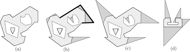
Figure 1: (a) A polygon $P$, where the polygon is filled and the holes are empty regions. (b) A subsuming polygon $P^{\prime}$, where $P^{\prime}$ is the union of the filled regions. A subsuming chain is shown in bold. (c) A min-convex subsuming polygon $P^{\prime}_{min}$, where $\mathcal{A}_{e}(P^{\prime}_{min})=\mathcal{A}_{e}(P)$. (d) A polygon $P$ such that for any min-convex subsuming polygon $P^{\prime}_{min}$, $\mathcal{A}_{e}(P)\not=\mathcal{A}_{e}(P^{\prime}_{min})$.

Aichholzer et al. [1] showed that for every polygon $P$ with $n$ vertices, $r>0$ of which are reflex, one can compute in linear time a subsuming polygon $P^{\prime}$ with at most $O(r)$ vertices. Note that although a subsuming polygon with $O(r)$ vertices always exists, no polynomial-time algorithm is known for computing a min-convex subsuming polygon. Finding an optimal subsuming polygon seems challenging since it does not always lie on the arrangement of lines $\mathcal{A}_{e}(P)$ (resp., $\mathcal{A}_{v}(P)$) determined by the edges (resp., pairs of vertices) of the input polygon. Figure 1(c) illustrates an optimal polygon $P^{\prime}_{min}$ for the polygon $P$ of Figure 1(a), where $\mathcal{A}_{e}(P^{\prime}_{min})=\mathcal{A}_{e}(P)$. On the other hand, Figure 1(d) shows that a min-convex subsuming polygon may not always lie on $\mathcal{A}_{e}(P)$ or $\mathcal{A}_{v}(P)$. Note that the input polygon of Figure 1(d) is a simple polygon, i.e., it does not contain any hole. Hence determining min-convex subsuming polygons seems challenging even for simple polygons. In fact, Aichholzer et al. [1] posed an open question that asks to determine the complexity of computing min-convex subsuming polygons, where the input is restricted to simple polygons.

Our contributions.

In this paper we show that the problem of computing a min-convex subsuming polygon is NP-hard for polygons possibly with holes (Section 2). We noted earlier that discretizing the solution space is a potential challenge, i.e., that the optimal polygon may not always lie on the line arrangement determined by the input polygon (Figure 1(d)). Interestingly, our NP-hardness result does not seem to utilize this challenge, instead, the hardness holds even when we restrict the subsuming chains to have constant length and to lie on $\mathcal{A}_{e}(P)$.

A question that naturally appears in this context is whether such restrictions on subsuming chains can make the problem easier for nontrivial classes of polygons. For example, consider an $x$-monotone polygon $P$, e.g., see Figure 2(a). Then it is not difficult to see that there exists a min-convex polygon such that each subsuming chain has constant length and lies on $\mathcal{A}_{e}(P)$. The argument is simple except for the subsuming chains that covers the two ends of $P$, e.g., see Figure 2(b). A simple proof is included in Section 3.

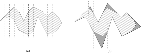
Figure 2: (a) An $x$-monotone polygon $P$. The dashed lines illustrate the monotonicity. (b) A min-convex subsuming polygon of $P$. The dashed lines illustrate the separation between successive chains.

We then show that the question can be answered affirmatively for arbitrary simple polygons, i.e., for any simple polygon $P$, one can compute in polynomial time, a min-convex subsuming polygon $P_{min}$ under the restriction that the subsuming chains are of constant length and lie on $\mathcal{A}_{e}(P)$.

Organization.

The rest of the paper is organized as follows. Section 2 presents the NP-hardness result for polygons with holes. Section 3 presents our observations on monotone polygons. Section 4 describes the techniques for computing subsuming polygons for simple polygons. Finally, Section 5 concludes the paper discussing directions to future research.

2 NP-hardness of Min-Convex Subsuming Polygon

In this section we prove that it is NP-hard to find a subsuming polygon with minimum number of convex vertices. We denote the problem by Min-Convex-Subsuming-Polygon. We reduce the NP-complete problem monotone planar 3-SAT [5], which is a variation of the 3-SAT problem as follows: Every clause in a monotone planar 3-SAT consists of either three negated variables (negative clause) or three non-negated variables (positive clause). Furthermore, the bipartite graph constructed from the variable-clause incidences, admits a planar drawing such that all the vertices corresponding to the variables lie along a horizontal straight line $l$, and all the vertices corresponding to the positive (respectively, negative) clauses lie above (respectively, below) $l$. The problem remains NP-hard even when each variable appears in at most four clauses [4].

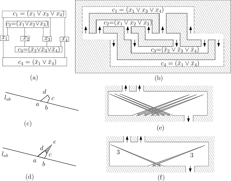
Figure 3: (a) An instance $I$ of monotone planar 3-SAT. (b) The orthogonal polygon $P_{o}$ corresponding to $I$. (c)–(f) Illustration for the variable gadget.

The idea of the reduction is as follows. Given an instance of a monotone planar 3-SAT $I$ with variable set $X$ and clause set $C$, we create a corresponding instance $\mathcal{P}_{I}$ of Min-Convex-Subsuming-Polygon. Let $\lambda$ be the number of convex vertices in $\mathcal{P}_{I}$. The reduction ensures that if there exists a satisfying truth assignment of $I$, then $\mathcal{P}_{I}$ can be subsumed by a polygon with at most $\lambda{-}|X||C|^{2}{-}3|C|$ convex vertices, and vice versa.

Given an instance $I$ of monotone planar 3-SAT, we first construct an orthogonal polygon $P_{o}$ with holes. We denote each clause and variable using a distinct axis-aligned rectangle, which we refer to as the c-rectangle and v-rectangle, respectively. Each edge connecting a clause and a variable is represented as a thin vertical strip, which we call an edge tunnel. Figures 3(a) and (b) illustrate an instance of monotone planar 3-SAT and the corresponding orthogonal polygon, respectively. While adding the edge tunnels, we ensure for each v-rectangle that the tunnels coming from top lie to the left of all the tunnels coming from the bottom. Figure 3(b) marks the top and bottom edge tunnels by upward and downward rays, respectively. The v-rectangles, c-rectangles and the edge tunnels may form one or more holes, as it is shown by diagonal line pattern in Figure 3. We now transform $P_{o}$ to an instance $\mathcal{P}_{I}$ of Min-Convex-Subsuming-Polygon.

We first introduce a few notations. Let $abcd$ be a convex quadrangle and let $l_{ab}$ be an infinite line that passes through $a$ and $b$. Assume also that $l_{bc}$ and $l_{ad}$ intersect at some point $e$, and $c,d,e$ all lie on the same side of $l_{ab}$, as shown in Figures 3(c)–(d). Then we call the quadrangle $abcd$ a tip on $l_{ab}$, and the triangle $cde$ a cap of $abcd$. The tip $abcd$ is called top-right, if the slope of $ad$ is positive; otherwise, it is called a top-left tip.

Variable gadget.

We construct variable gadgets from the v-rectangles. We add some top-right (and the same number of top-left) tips at the bottom side of the v-rectangle, as show in Figure 3(e). There are three top-right and top-left tips in the figure. For convenience we show only one top-left and one top-right tip in the schematic representation, as shown in Figure 3(f). However, we assign weight to these tips to denote how many tips there should be in the exact construction. We will ensure a few more properties: (I) The caps do not intersect the boundary of the v-rectangle, (II) no two top-left caps (or, top-right caps) intersect, and (III) every top-left (resp., top-right) cap intersects all the top-right (resp., top-left) caps.

Observe that each top-left tip contributes to two convex vertices such that covering them with a cap reduces the number of convex vertices by 1. The peak of the cap reaches very close to the top-left corner of the v-rectangle, which will later interfere with the clause gadget. Specifically, this cap will intersect any downward cap of the clause gadget coming through the top edge tunnels. Similarly, each top-right tip contributes to two convex vertices, and the corresponding cap intersects any upward cap coming through the bottom edge tunnels.

Note that the optimal subsuming polygon $P$ cannot contain the caps from both the top-left and top-right tips. We assign the tips with a weight of $|C|^{2}$. In the hardness proof this will ensure that either the caps of top-right tips or the caps of top-left tips must exist in $P$, which will correspond to the true and false configurations, respectively.

Clause gadget.

Recall that, by definition, each clause consists of three variables and so it is incident to three edge tunnels. Figure 4(a) illustrates the transformation for a c-rectangle. Here we describe the gadget for the positive clauses, and the construction for negative clauses is symmetric. We add three downward tips incident to the top side of the c-rectangle, along its three edge tunnels. Each of these downward tip contributes to two convex vertices such that covering the tip with a cap reduces the number of convex vertices by 1. Besides, the corresponding caps reach almost to the bottom side of the v-rectangles, i.e., they would intersect the top-left caps of the $v$-rectangles. Let these tips be $t_{1},t_{2},t_{3}$ from left to right, and let $\gamma_{1},\gamma_{2},\gamma_{3}$ be the corresponding caps.

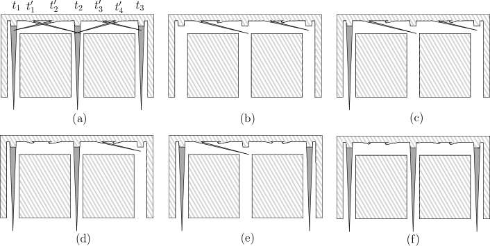
Figure 4: Illustration for the clause gadget.

We then add a down-left and a down-right tip at the top side of the $c$-rectangle between $t_{i}$ and $t_{i+1}$, where $1\leq i\leq 2$, as shown in Figure 4(a). Let the tips be $t^{\prime}_{1},\ldots,t^{\prime}_{4}$ from left to right, and let the corresponding caps be $\gamma^{\prime}_{1},\ldots,\gamma^{\prime}_{4}$. Note that the caps corresponding to $t^{\prime}_{j}$ and $t^{\prime}_{j+1}$, where $j\in\{1,3\}$, intersect each other. Therefore, at most two of these four caps can exist at the same time in the solution polygon. Observe also that the caps corresponding to $t_{1},t_{2},t_{3}$ intersect the caps corresponding to $\{t^{\prime}_{2}\},\{t^{\prime}_{1},t^{\prime}_{4}\},\{t^{\prime}_{3}\}$, respectively. Consequently, any optimal solution polygon containing none of $\{\gamma_{1},\gamma_{2},\gamma_{3}\}$ has at least 12 convex vertices along the top boundary of the c-rectangle, as shown in Figure 4(b).

We now show that any optimal solution polygon $P$ containing at least $\alpha>0$ caps from $\Gamma=\{\gamma_{1},\gamma_{2},\gamma_{3}\}$ have exactly 11 convex vertices along the top boundary of the c-rectangle. We consider the following three cases:

Case 1 ($\alpha=1$): If $\gamma_{1}$ (resp., $\gamma_{3}$) is in $P$, then $P$ must contain $\{\gamma^{\prime}_{1},\gamma^{\prime}_{3}\}$ (resp., $\{\gamma^{\prime}_{2},\gamma^{\prime}_{4}\}$). Figure 4(c) illustrates the case when $P$ contains $\gamma_{1}$. If $\gamma_{2}$ is in $P$, then $P$ must contain $\{\gamma^{\prime}_{2},\gamma^{\prime}_{3}\}$. In all the above scenarios the number of convex vertices along the top boundary of the c-rectangle is 11.

Case 2 ($\alpha=2$): If $P$ contains $\{\gamma_{1},\gamma_{3}\}$, then either $\gamma^{\prime}_{1}$ or $\gamma^{\prime}_{4}$ must be in $P$. Otherwise, $P$ contains either $\{\gamma_{1},\gamma_{2}\}$ or $\{\gamma_{2},\gamma_{3}\}$. If that $P$ contains $\{\gamma_{1},\gamma_{2}\}$, as in Figure 4(d), then $\gamma^{\prime}_{3}$ must lie in $P$. In the remaining case, $\gamma^{\prime}_{2}$ must lie in $P$. Therefore, also in this case the number of convex vertices along the top boundary of the c-rectangle is 11.

Case 3 ($\alpha=3$): In this scenario $P$ cannot contain any of $\gamma^{\prime}_{1},\ldots,\gamma^{\prime}_{4}$. Therefore, as shown in Figure 4(e), the number of convex vertices along the top boundary of the c-rectangle is 11.

As a consequence we obtain the following lemma.

Lemma 2.1.

If a clause is satisfied, then any optimal subsuming polygon reduces exactly three convex vertex from the corresponding c-rectangle.

Reduction.

Although we have already described the variable and clause gadgets, the optimal subsuming polygon still may come up with some unexpected optimization that interferes with the convex corner count in our hardness proof. Figure 5(left) illustrates one such example. Therefore, we replace each convex corner that does not correspond to the tips by a small polyline with alternating convex and reflex corners, as shown Figure 5(right). By construction, it is now straightforward to observe the following fact.

Remark 1.

Let $r$ be a reflex vertex of $\mathcal{P}_{I}$, and let $r^{\prime}$ be the first reflex vertex after $r$ while walking clockwise on the boundary of $\mathcal{P}_{I}$ starting at $r$. Then the number of convex vertices that can appear between $r$ and $r^{\prime}$ is at most two. Furthermore, if there are two convex vertices, then either they correspond to a tip, or form an $180^{\circ}$ turn using only orthogonal line segments.

We now prove the NP-hardness of computing an optimal subsuming polygon.

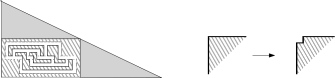
Figure 5: Refinement of $\mathcal{P}_{I}$.

Theorem 2.1.

Finding an optimal subsuming polygon is NP-hard.

Proof.

Let $I=(X,C)$ be an instance of monotone planar 3-SAT and let $\mathcal{P}_{I}$ be the corresponding instance of Min-Convex-Subsuming-Polygon. Let $\lambda$ be the number of convex vertices in $\mathcal{P}_{I}$. We now show that $I$ admits a satisfying truth assignment if and only if $\mathcal{P}_{I}$ can be subsumed using a polygon having at most $\lambda-|X||C|^{2}-3|C|$ convex vertices.

First assume that $I$ admits a satisfying truth assignment. For each variable $x$, we choose either the top-right caps or the top-left caps depending on whether $x$ is assigned true or false. Consequently, we save at least $|X||C|^{2}$ convex vertices. Consider any clause $c\in C$. Since $c$ is satisfied, one or more of its variables are assigned true. Therefore, for each positive (resp., negative) clause, we can have one or more downward (resp., upward) caps that enter into the v-rectangles. By Lemma 2.1, we can save at least three convex vertices from each c-rectangle. Therefore, we can find a subsuming polygon with at most $\lambda-|X||C|^{2}-3|C|$ convex vertices.

Assume now that some polygon $P$ with at most $\lambda-|X||C|^{2}-3|C|$ convex vertices can subsume $\mathcal{P}_{I}$. We now find a satisfying truth assignment for $I$. By Remark 1 we can restrict our attention only to c- and v-rectangles. Note that the maximum number of convex vertices that can be reduced from the c-rectangles is at most $3|C|$. Therefore, $P$ must reduce at least $|C|^{2}$ convex vertices from each v-rectangle. Recall that in each v-rectangle, either the top-right or the top-left caps can be chosen in the solution, but not both. Therefore, the v-rectangles cannot help reducing more than $|X||C|^{2}$ convex vertices. If $P$ contains the top-right caps of the v-rectangle, then we set the corresponding variable to true, otherwise, we set it to false. Since $P$ has at most $\lambda-|X||C|^{2}-3|C|$ convex vertices, and each c-rectangle can help to reduce at most $3$ convex vertices (Lemma 2.1), $P$ must have at least one cap from $\gamma_{1},\gamma_{2},\gamma_{3}$ at each c-rectangle. Therefore, each clause must be satisfied. Recall that the downward (resp., upward) caps coming from edge tunnels are designed carefully to have conflict with the top-left (resp., top-right) caps of v-variables. Since top-left and top-right caps of v-variables are conflicting, the truth assignment of each variable is consistent in all the clauses that contains it. ∎

It is straightforward from the construction of $\mathcal{P}_{I}$ that no optimal subsuming polygon $P$ that subsumes $\mathcal{P}_{I}$ can have a subsuming chain of length larger than 3, and there always exists an optimal solution that lies on $\mathcal{A}_{e}(\mathcal{P}_{I})$. Hence, Theorem 2.1 holds even under the restriction that the subsuming chains must be of constant length and lie on $\mathcal{A}_{e}(\mathcal{P}_{I})$. In Sections 3 and 4, we will show that these restrictions make the problem polynomial-time solvable for simple polygons.

3 Monotone Polygons

In this section, we give a straightforward algorithm to compute a min-convex subsuming polygon of $x$-monotone polygons. In fact, we prove a stronger claim that every $x$-monotone polygon $P$ admits a min-convex subsuming polygon such that the subsuming chains are of constant length and lie on $\mathcal{A}_{e}(P)$.

Let $\texttt{upper}(P)$ and $\texttt{lower}(P)$ denote the upper and lower chains of $P$, respectively. Moreover, let $u_{1}$ (resp., $u_{m}$) be the leftmost (resp., rightmost) vertex of $P$; notice that the vertices $u_{1}$ and $u_{m}$ are both convex (as $P$ is $x$-monotone) and are shared between $\texttt{upper}(P)$ and $\texttt{lower}(P)$. Let $u_{2},\dots,u_{m-1}$ (resp., $l_{2},\dots,l_{m^{\prime}-1}$) be the set of reflex vertices of $P$ that lie on $\texttt{upper}(P)$ (resp., on $\texttt{lower}(P)$); we let $l_{1}=u_{1}$ and $l_{m^{\prime}}=u_{m}$. For a reflex vertex $u_{i}$, where $2\leq i<m$, let $\ell^{-}(u_{i})$ (resp., $\ell^{+}(u_{i})$) denote the line determined by the edge $(u_{i-1},u_{i})$ (resp., $(u_{i},u_{i+1})$). Similarly, define the lines $\ell^{-}(l_{i})$ and $\ell^{+}(l_{i})$ for all $2\leq i<m^{\prime}$. For $u_{1}$ and $u_{m}$, only $\ell^{+}(u_{1})$ and $\ell^{-}(u_{m})$ are defined. We next describe the algorithm.

First, consider $\texttt{upper}(P)$. Initially, let the simplified polygon $P^{\prime}$ be $P$. For each reflex vertex $u_{i}$ on $\texttt{upper}(P)$, where $2\leq i<m-1$, consider the vertical slab defined by the two vertical lines through $u_{i}$ and $u_{i+1}$. If there is no convex vertex of $\texttt{upper}(P)$ in this slab, then the edge $u_{i}u_{i+1}$ must be an edge of any feasible solution. So, such an edge stays in $P^{\prime}$. Otherwise, $\ell^{+}(u_{i})$ and $\ell^{-}(u_{i+1})$ intersect each other at some point $p$ outside and above $P$ or on $P$. Then, we remove the chain of convex vertices between $u_{i}$ and $u_{i+1}$ and add the two edges $u_{i}p$ and $u_{i+1}p$ to $P^{\prime}$; hence, reducing the number of convex vertices of $\texttt{upper}(P)$ between $u_{i}$ and $u_{i+1}$ to one. Next, we consider $\texttt{lower}(P)$ and apply the same process to every two each vertex $l_{i}$ on $\texttt{lower}(P)$, where $2\leq i<m^{\prime}-1$.

It remains to show how to deal with the convex vertices that appear before the leftmost reflex vertex or after the rightmost reflex vertex on each chain. We show that these convex vertices can be reduced to at most two convex vertices, depending on the slopes of the edges incident to such reflex vertices. In the following, as the second part of the algorithm, we discuss the details for convex vertices that appear before the leftmost reflex vertices; the convex vertices on the other end of the polygon can be handled similarly.

Consider $u_{1}$ (i.e., the leftmost vertex of $P$) and let $u_{r}$ and $l_{r}$ denote the leftmost reflex vertices on $\texttt{upper}(P)$ and $\texttt{lower}(P)$, respectively. Let $\pi$ be the chain on the boundary of $P$ that connects $u_{r}$ to $l_{r}$ in counter-clockwise order (i.e., it contains $u_{1}$). To reduce the number of convex vertices on $\pi$, it is sufficient to check if $\ell^{-}(u_{r})$ and $\ell^{-}(l_{r})$ intersect at some point $p$ whose $x$-coordinate is less than that of both $u_{r}$ and $l_{r}$. For instance, if the slope of $\ell^{-}(u_{r})$ is positive and the slope of $\ell^{-}(l_{r})$ is negative, then $\ell^{-}(u_{r})$ and $\ell^{-}(l_{r})$ intersect at such point $p$; see Figure 6(a). In this case, we can replace $\pi$ with two edges $u_{r}p$ and $l_{r}p$; hence, reducing the number of convex vertices on $\pi$ to one. Therefore, we can simplify $\pi$ as follows: if $\ell^{-}(u_{r})$ and $\ell^{-}(l_{r})$ intersect at such point $p$, then we replace $\pi$ with two edges $u_{r}p$ and $l_{r}p$ (hence, reducing the number of convex vertices on $\pi$ to one). Otherwise, if no such point $p$ exists (e.g., when the slope of $\ell^{-}(u_{r})$ is negative, but the slope of $\ell^{-}(l_{r})$ is positive), then both $\ell^{-}(u_{r})$ and $\ell^{-}(l_{r})$ must intersect the line passing through at least one of the edges incident to $u_{1}$. See Figure 6(b-c). So, we can replace $\pi$ with three edges and reducing the convex vertices on $\pi$ to two. We perform a similar reduction on the path $\pi$ corresponding to the rightmost convex vertex of $P$ and its “closest” reflex vertices from each chain on the other end of $P$. Let $P^{*}$ be the resulting simplified polygon.

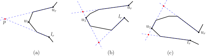
Figure 6: How to reduce the convex vertices around the leftmost vertex $u_{1}$ of $P$.

To see the monotonicity of $P^{*}$, we note that in each slab considered in the first part of the algorithm, at most two new edges are introduced that lie inside the slab. Therefore, the edges from different slabs are disjoint. Moreover, the edges introduced in the second part of the algorithm (i.e., when dealing with the leftmost and rightmost convex vertices $u_{1}$ and $u_{m}$) do not violate the monotonicity of $P^{*}$.

For every two consecutive reflex vertices, $P^{*}$ has exactly one convex vertex (resp., has no convex vertex) between them if $P$ had at least one (resp., had none) between them. Since there must be at least one convex vertex between every two reflex vertices that had at least one convex vertex between them, any simplified polygon must have at least as many convex vertices as $P^{*}$ between every two consecutive reflex vertices. Moreover, one can easily verify that $P^{*}$ has the minimum number of convex vertices generated in the second part of the algorithm. Therefore, $P^{*}$ is optimal and we hence have the following result.

Theorem 3.1.

Given a monotone polygon $P$ with $n$ vertices, a subsuming polygon of $P$ with the minimum number of convex vertices can be computed in $O(n\log n)$ time.

4 Computing Subsuming Polygons

In this section, we show that for any simple polygon $P$, a min-convex subsuming polygon $P_{min}$ can be computed in polynomial time under the restriction that the subsuming chains are of constant length and lie on $\mathcal{A}_{e}(P)$. We first present definitions and preliminary results on outerstring graphs, which will be an important tool for computing subsuming polygons.

Independent set in outerstring graphs.

A graph $G$ is a string graph if it is an intersection graph of a set of simple curves in the plane, i.e., each vertex of $G$ is a mapped to a curve (string), and two vertices are adjacent in $G$ if and only if the corresponding curves intersect. $G$ is an outerstring graph if the underlying curves lie interior to a simple cycle $C$, where each curve intersects $C$ at one of its endpoints. Figure 7(a) illustrates an outerstring graph and the corresponding arrangement of curves. Later in our algorithm, the polygon will correspond to the cycle of an outerstring graph, and some polygonal chains attached to the boundary of the polygon will correspond to the strings of that outerstring graph.

A set of strings is called independent if no two strings in the set intersect, the corresponding vertices in $G$ are called an independent set of vertices. Let $G$ be a weighted outerstring graph with a set $\mathcal{T}$ of weighted strings. A maximum weight independent set $\mathtt{MWIS}(\mathcal{T})$ (resp., $\mathtt{MWIS}(G)$) is a set of independent strings $T\subseteq\mathcal{T}$ (resp., vertices) that maximizes the sum of the weights of the strings in $T$. By $|\mathtt{MWIS}(G)|$ we denote the weight of $\mathtt{MWIS}(G)$.

Let $\Gamma(G)$ be the arrangement of curves that corresponds to $G$; e.g., see Figure 7(a). Let $R$ be a geometric representation of $\Gamma(G)$, where $C$ is represented as a simple polygon $P$, and each curve is represented as a simple polygonal chain inside $P$ such that one of its endpoints coincides with a distinct vertex of $P$. Keil et al. [8] showed that given a geometric representation $R$ of $G$, one can compute a maximum weight independent set of $G$ in $O(s^{3})$ time, where $s$ is the number of line segments in $R$.

Theorem 4.1 (Keil et al. [8]).

Let $G$ be a weighted outerstring graph. Given a geometric representation $R$ of $G$, there exists a dynamic programming algorithm that computes a maximum weight independent set of $G$ in $O(s^{3})$ time, where $s$ is the number of straight line segments in $R$.

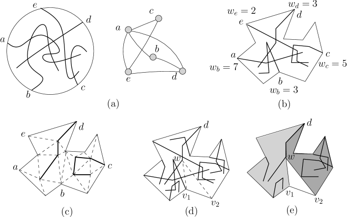
Figure 7: (a) Illustration for $G$ and $\Gamma(G)$. (b) A geometric representation $R$ of $G$. (c) A triangulated polygon obtained from an independent set of $G$. (d)–(e) Dynamic programming to find maximum weight independent set.

Figure 7(b) illustrates a geometric representation $R$ of some $G$, where each string is represented with at most 4 segments. Keil et al. [8] observed that any maximum weight independent set of strings can be triangulated to create a triangulation $P_{t}$ of $P$, as shown in Figure 7(c). They used this idea to design a dynamic programming algorithm, as follows. Let $\mathcal{T}$ be the strings in $R$. Then the problem of finding $\mathtt{MWIS}(\mathcal{T})$ can be solved by dividing the problem into subproblems, each described using only two points of $R$. We illustrate how the subproblems are computed very briefly using Figure 7(d). Let $P(v_{1},v_{2})$ be the problem of finding $\mathtt{MWIS}(\mathcal{T}_{v_{1},v_{2}})$, where $\mathcal{T}_{v_{1},v_{2}}$ consists of the strings that lie to the left of $v_{1}v_{2}$. Let $wv_{1}v_{2}$ be a triangle in $P_{t}$, where $w$ is a point on some string $d$ inside $P(v_{1},v_{2})$; see Figure 7(d). Since $P_{t}$ is a triangulation of the maximum weight string set, $d$ must be a string in the optimal solution. Hence $P(v_{1},v_{2})$ can be computed from the solution to the subproblems $P(v_{1},w)$ and $P(w,v_{2})$, as shown in Figure 7(e). Keil et al. [8] showed that there are only a few different cases depending on whether the points describing the subproblems belong to the polygon or the strings. We will use this idea of computing $\mathtt{MWIS}(\mathcal{T})$ to compute subsuming polygons.

Subsuming polygons via outerstring graphs.

Let $P=(v_{0},v_{1},\ldots,v_{n-1})$ be a simple polygon with $n$ vertices, $r>0$ of which are reflex vertices. A convex chain of $P$ is a path $C_{ij}=(v_{i},v_{i+1},\ldots,v_{j-1},v_{j})$ of strictly convex vertices, where the indices are considered modulo $n$.

Let $P^{\prime}=(w_{0},w_{1},\ldots,w_{m-1})$ be a subsuming polygon of $P$, where $\mathcal{A}_{e}(P^{\prime})=\mathcal{A}_{e}(P)$, and the subsuming chains are of length at most $t$. Here, by “length”, we mean the number of edges (not the Euclidean length). Let $C^{\prime}_{qr}=(w_{q},\ldots,w_{r})$ be a subsuming chain of $P^{\prime}$. Then by definition, there is a corresponding convex chain $C_{ij}$ in $P$ such that the edges $(v_{i},v_{i+1})$ and $(v_{j-1},v_{j})$ coincide with the edges $(w_{q},w_{q+1})$ and $(w_{r-1},w_{r})$. We call the vertex $v_{i}$ the left support of $C^{\prime}_{qr}$. Since $\mathcal{A}_{e}(P^{\prime})=\mathcal{A}_{e}(P)$, the chain $C^{\prime}_{qr}$ must lie on $\mathcal{A}_{e}(P)$. Moreover, since $P^{\prime}$ is a min-convex subsuming polygon, the number of vertices in $C^{\prime}_{qr}$ would be at most the number of vertices in $C_{ij}$.

We claim that the number of paths in $\mathcal{A}_{e}(P)$ from $v_{i}$ to $v_{j}$ is at most $n^{t}$, where $t=O(1)$ is an upper bound on the length of the subsuming chains. Thus any subsuming chain can have at most $(t-1)$ line segments. Since there are only $O(n)$ straight lines in the arrangement $\mathcal{A}_{e}(P)$, there can be at most $n^{j}$ paths of $j$ edges, where $1\leq j\leq t-1$. Consequently, the number of candidate chains that can subsume $C_{ij}$ is $O(n^{t})$.

Lemma 4.1.

Given a simple polygon $P$ with $n$ vertices, every convex chain $C$ of $P$ has at most $O(n^{t})$ candidate subsuming chains in $\mathcal{A}_{e}(P)$, each of length at most $t$.

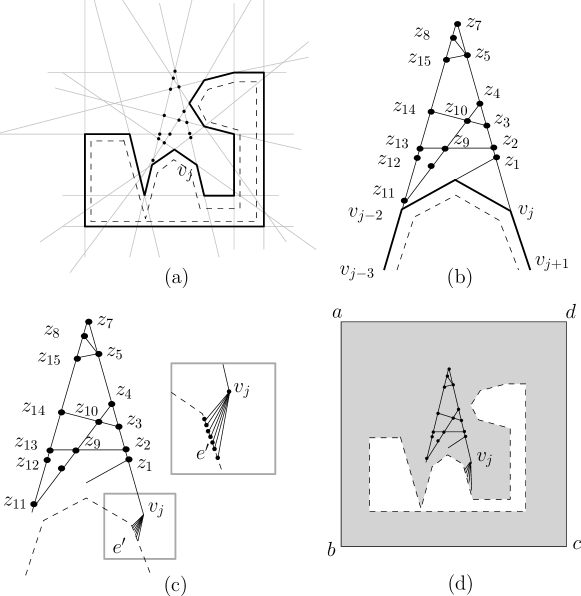
Figure 8: (a) Illustration for the polygon $P$ (in bold), $\mathcal{A}_{e}(P)$ (in gray), and $Q$ (in dashed lines). (b) Chains of $v_{j}$. (c) Attaching the strings to $Q$. (d) Dynamic programming inside the gray region.

In the following, we construct an outerstring graph using these candidate subsuming chains. We first compute a simple polygon $Q$ interior to $P$ such that for each edge $e$ in $P$, there exists a corresponding edge $e^{\prime}$ in $Q$ which is parallel to $e$ and the perpendicular distance between $e$ and $e^{\prime}$ is $\epsilon$, as shown in dashed line in Figure 8(a). We choose $\epsilon$ sufficiently small such that for each component $w$ of $P$, $Q$ contains exactly one component inside $w$. We now construct the strings. Let $v_{j}$ be a convex corner of $P$. Let $S_{j}$ be the set of candidate subsuming chains such that for each chain in $S_{j}$, the left support of the chain appears before $v_{j}$ while traversing the unbounded face of $P$ in clockwise order. For example, the subsuming chains that correspond to $v_{j}$ are $(v_{j-2},z_{1},v_{j+1})$, $(v_{j-3},z_{13},z_{2},v_{j+1})$, $(v_{j-3},z_{14},z_{3},v_{j+1})$, $(v_{j-3},z_{11},z_{4},v_{j+1})$, $(v_{j-3},z_{15},z_{5},v_{j+1})$, $(v_{j-3},z_{8},z_{5},v_{j+1})$, $(v_{j-3},z_{7},v_{j+1})$, as shown in Figure 8(b). For each of these chains, we create a unique endpoint on the edge $e^{\prime}$ of $Q$, where $e^{\prime}$ corresponds to the edge $v_{j}v_{j+1}$ in $P$, as shown in Figure 8(c). We then attach these chains to $Q$ by adding a segment from $v_{j}$ to its unique endpoint on $Q$.

We attach the chains for all the convex vertices of $P$ to $Q$. Later we will use these chains as the strings of an outerstring graph. We then assign each chain a weight, which is the number of convex vertices of $P$ it can reduce. For example in Figure 8(b), the weight of the chain $(v_{j-3},z_{8},z_{5},v_{j+1})$ is one.

Although the strings are outside of the simple cycle, it is straightforward to construct a representation with all the strings inside a simple cycle $Q$: Consider placing a dummy vertex at the intersection points of the arrangement, and then find a straight-line embedding of the resulting planar graph such that the boundary of $Q$ corresponds to the outer face of the embedding. Consequently, $Q$ and its associated strings correspond to an outerstring graph representation $R$. Let $G$ be the underlying outerstring graph. We now claim that any $\mathtt{MWIS}(G)$ corresponds to a min-convex subsuming polygon of $P$.

Lemma 4.2.

Let $P$ be a simple polygon, where there exists a min-convex subsuming polygon that lies on $\mathcal{A}_{e}(P)$, and let $G$ be the corresponding outerstring graph. Any maximum weight independent set of $G$ yields a min-convex subsuming polygon of $P$.

Proof.

Let $T$ be a set of strings that correspond to a maximum weight independent set of $G$. Since $T$ is an independent set, the corresponding subsuming chains do not create edge crossings. Moreover, since each subsuming chain is weighted by the number of convex corners it can remove, the subsuming chains corresponding to $T$ can remove $|\mathtt{MWIS}(G)|$ convex corners in total.

Assume now that there exists a min-convex subsuming polygon that can remove at least $k$ convex corners. The corresponding subsuming chains would correspond to an independent set $T^{\prime}$ of strings in $G$. Since each string is weighted by the number of convex corners the corresponding subsuming chain can remove, the weight of $T^{\prime}$ would be at least $k$. ∎

Time complexity.

To construct $G$, we first placed a dummy vertex at the intersection points of the chains, and then computed a straight-line embedding of the resulting planar graph such that all the vertices of $Q$ are on the outerface. Therefore, the geometric representation used at most $nt$ edges to represent each string. Since each convex vertex of $P$ is associated with at most $O(n^{t})$ strings, there are at most $n\times O(n^{t})$ strings in $G$. Consequently, the total number of segments used in the geometric representation is $O(tn^{2+t})$. A subtle point here is that the strings in our representation may partially overlap, and more than three strings may intersect at one point. Removing such degeneracy does not increase the asymptotic size of the representation. Finally, by Theorem 4.1, one can compute the optimal subsuming polygon in $O(t^{3}n^{6+3t})$ time.

The complexity can be improved further as follows. Let $abcd$ be a rectangle that contains all the intersection points of $\mathcal{A}_{e}(P)$. Then, every optimal solution can be extended to a triangulation of the closed region between $abcd$ and $Q$. Figure 8(d) illustrates this region in gray. We can now apply dynamic programming similar to the one described above to compute the maximum weight independent string set, where each subproblem finds a maximum weight set inside some subpolygon. Each such subpolygon can be described using two points $v_{1},v_{2}$, each lying either on $Q$ or on some string, and a subset of $\{a,b,c,d\}$ that helps enclosing the subpolygon.

Since there are $n\times O(n^{t})$ strings, each containing at most $t$ points, the number of vertices that correspond to the strings is $O(tn^{1+t})$. We will refer these as the string vertices. Note that the number of total vertices in the geometric representation is also $O(tn^{1+t})$. If the subproblem is bounded by two string vertices, or one string vertex and one polygon vertex, then similar to Keil et al. [8], we can use a pair of vertices to describe a subproblem. However, sometimes we need more information to describe a subproblem, e.g., assume that the subproblem is bounded from one side by the point $a$ and some vertex $v$ (corresponding to a string), and from the other side by the point $d$ and some vertex $v^{\prime}$ (corresponding to a string). For these problems, we need a subset of $\{a,b,c,d\}$ to describe the problem boundary. Therefore, we define our dynamic programing table to be $\mathcal{D}[x,y,z]$, where $x$ and $y$ corresponds to the string or polygon vertices, and $z$ corresponds to the constant size additional description of the boundary (whenever needed). Thus the size of the dynamic programming table is $O(tn^{1+t})\times O(tn^{1+t})\times O(1)$. Since there are at most $O(tn^{1+t})$ string vertices, there can be at most $O(tn^{1+t})$ candidate triangles $v_{1}v_{2}w$ (e.g., Figure 7 (e)). Consequently, we can fill an entry of the table in $O(tn^{1+t})$ time. Hence the dynamic program takes at most $O(t^{3}n^{3+3t})$ time in total.

Theorem 4.2.

Given a simple polygon $P$ with $n$ vertices, one can compute in polynomial time, a min-convex subsuming polygon under the restriction that the subsuming chains must be of constant length and lie on $\mathcal{A}_{e}(P)$.

Generalizations.

We can further generalize the results for any given line arrangements. However, such a generalization may increase the time complexity. For example, consider the case when the given line arrangement is $\mathcal{A}_{v}(P)$, which is determined by the pairs of vertices of $P$. Since we now have $O(n^{2})$ lines in the arrangement $\mathcal{A}_{v}(P)$, the time complexity increases to $O(t^{3}(n^{2})^{3+3t})$, i.e., $O(t^{3}n^{6+6t})$.

5 Conclusion

In this paper, we developed a polynomial-time algorithm that can compute optimal subsuming polygons for a given simple polygon in restricted settings. On the other hand, if the polygon contains holes, then we showed that the problem of computing an optimal subsuming polygon is NP-hard. Therefore, the question of whether the problem is polynomial-time solvable for simple polygons [1], remains open. Note that islands are crucial in our hardness proof. The complexity of the problem for polygons with holes (but without any island) is also open. Since the optimization in one hole is independent of the optimization in the other holes of the polygon, resolving the complexity for polygon with holes would readily give important insight about the complexity for simple polygon.

Our algorithm can find an optimal solution if the optimal subsuming polygon lies on some prescribed arrangement of lines, e.g., $\mathcal{A}_{e}(P)$ or $\mathcal{A}_{v}(P)$. The running time of our algorithm depends on the length of the subsuming chains, i.e., the running time is polynomial if the subsuming chains are of constant length. However, there exist polygons whose optimal subsuming polygons contain subsuming chains of length $\Omega(n)$. Figure 9 illustrates such an example optimal solution that is lying on $\mathcal{A}_{e}(P)$. An interesting research direction would be to examine whether there exists a good approximation algorithm for the general problem.

Recently, Lubiw et al. [9] showed that the problem of drawing a graph inside a polygonal region is hard for the existential theory of the reals. The subsuming polygon problem can also be viewed as a constrained graph drawing problem whereas the subsuming chains are modeled by edges that need to be drawn outside the polygon, possibly with bends. The goal is to find a crossing-free drawing of these edges that minimizes the total number of bends. It would be interesting to examine whether the problem is $\exists\mathbb{R}$-hard in such a graph drawing model.

Figure 9: Illustration for the case when the optimal subsuming polygon contains a subsuming chain of length $\Omega(n)$. The subsuming chain is shown in bold.

References

- [1] O. Aichholzer, T. Hackl, M. Korman, A. Pilz, and B. Vogtenhuber. Geodesic-preserving polygon simplification. International Journal of Computational Geometry & Applications, 24(4):307–324, 2014.
- [2] L. Arge, L. Deleuran, T. Mølhave, M. Revsbæk, and J. Truelsen. Simplifying massive contour maps. In Proc. ESA, volume 7501 of LNCS, pages 96–107. Springer, 2012.
- [3] Y. Bahoo, S. Durocher, J. M. Keil, S. Mehrabi, S. Mehrpour, and D. Mondal. Polygon simplification by minimizing convex corners. In Thang N. Dinh and My T. Thai, editors, Proceedings of the 22nd International Conference on Computing and Combinatorics (COCOON), volume 9797 of LNCS, pages 547–559. Springer, 2016.
- [4] A. Darmann, J. Döcker, and B. Dorn. On planar variants of the monotone satisfiability problem with bounded variable appearances, 2016. https://arxiv.org/abs/1604.05588.
- [5] M. de Berg and A. Khosravi. Optimal binary space partitions for segments in the plane. International Journal of Computational Geometry & Applications, 22(3):187–206, 2012.
- [6] D. H. Douglas and T. K. Peucker. Algorithm for the reduction of the number of points required to represent a line or its caricature. The Canadian Cartographer, 10(2):112–122, 1973.
- [7] L. J. Guibas, J. Hershberger, J. S. B. Mitchell, and J. Snoeyink. Approximating polygons and subdivisions with minimum link paths. International Journal of Computational Geometry & Applications, 3(4):383–415, 1993.
- [8] J. Mark Keil, Joseph S. B. Mitchell, Dinabandhu Pradhan, and Martin Vatshelle. An algorithm for the maximum weight independent set problem on outerstring graphs. Computational Geometry, 60:19–25, 2017.
- [9] A. Lubiw, T. Miltzow, and D. Mondal. The complexity of drawing a graph in a polygonal region. CoRR, abs/1802.06699, 2018.
- [10] W. A. Mackaness, A. Ruas, and L. Tiina Sarjakoski. Generalisation of Geographic Information: Cartographic Modelling and Applications. Elsevier, 2011.
- [11] H. Ratschek and J. Rokne. Geometric Computations with Interval and New Robust Methods: Applications in Computer Graphics, GIS and Computational Geometry. Horwood Publishing, 2003.