A Simple Method for 5G Positioning and Synchronization without Line-of-Sight

Abstract

In 5G mmWave, joint positioning and synchronization can be achieved even when the line-of-sight (LOS) path is blocked. In this technical note, we describe a simple method to determine a coarse estimate of the user state and the environment. This method is based on geometric consistency of the 5G mmWave measurements and can be used as a pre-processor for other more sophisticated methods, in order to reduce their complexity. A link to MATLAB source code is provided at the end of the document.

I Introduction

In 5G positioning, a received signal can carry information in the delay and angle domain [1]. A common model of a received signal is

$$\mathbf{y}(t)=\mathbf{W}^{\text{H}}\sum_{l=0}^{L}h_{l}\mathbf{a}_{\text{R}}(\bm{\theta}_{l})\mathbf{a}_{\text{T}}^{\text{H}}(\bm{\phi}_{l})\mathbf{s}(t-\tau_{l})+\mathbf{n}(t),$$ (1)

where $\mathbf{s}(t)$ is a transmitted signal (possibly precoded), $\mathbf{W}$ is a combining matrix, $h_{l}$ is a complex path gain, $\bm{\theta}_{l}$ is the angle of arrival (AOA) in azimuth and elevation, $\bm{\phi}_{l}$ is the angle of departure (AOD) in azimuth and elevation, $\tau_{l}$ is the time of arrival (TOA), and $\mathbf{n}(t)$ is (possibly colored) noise. The AOA and TOA are measured in the frame of reference of the receiver, while the AOD is measured in the frame of reference of the transmitter. The path index $l=0$ is the line-of-sight (LOS) path, while the $L$ remaining paths are non-LOS (NLOS) paths.

The AOA, TOA, and AOD of each path has a geometric meaning, which depends on the location of the transmitter and receiver, as well as the points of incidence of the NLOS paths in the environment (see further). We will consider a downlink scenario, where the transmitting base station (BS) has a known position, $\mathbf{x}_{\text{BS}}\in\mathbb{R}^{3}$, the user equipment (UE) has an unknown position $\mathbf{x}\in\mathbb{R}^{3}$, as well as an unknown clock bias $B$ (expressed in meters) and an unknown orientation $\alpha$ with respect to the vertical axis. Moreover, the unknown incidence points of the NLOS paths in the environment are denoted by $\mathbf{x}_{s,l}\in\mathbb{R}^{3}$. These incidence points or scattering points (SPs) could be related to reflecting surfaces or small scattering objects. We further assume a channel estimation routine is present at the receiver, which provides

$$\mathbf{z}_{l}=[\tau_{l}\,\bm{\theta}_{l}^{\text{T}},\bm{\phi}_{l}^{\text{T}}]^{\text{T}}+\mathbf{w}_{l},\,\mathbf{w}_{l}\sim\mathcal{N}(\mathbf{0},\bm{\Sigma}_{l}).$$ (2)

Our objective is now, given these measurements, to determine $\mathbf{x}$, $\alpha$, $B$, $\{\mathbf{x}_{s,l}\}_{l=1}^{L}$ with only minimal prior information (the communication range $R$ between transmitter and receiver) and in the absence of the LOS path (i.e., the path $l=0$ is not present, e.g., due to obstacles).

I-A Related Works

Similar problems were considered without $B$ in [1], where an exhaustive search over $\alpha$ was performed and for each trial value a least-squares problems was solved to find an estimate of $\mathbf{x}$ and $\{\mathbf{x}_{s,l}\}_{l=1}^{L}$. The estimate with the lowest cost was then retained. In [2] a Gibbs sampling approach was proposed, where first a sample of the UE position and orientation was generated from a prior density, followed by sampling the SPs, and so forth. In [3], a factor graph method was proposed where particles are used to represent the uncertainties of the unknown variables. For high measurement variance, this method proved more robust than [1]. While there are many other works that relate to the problem at hand, only those above consider the NLOS-only case. When the LOS is present the problem becomes significantly more tractable (provided it is known which path is the LOS path). When the LOS is absent and the transmitter and receiver are not synchronized, the problem becomes significantly harder: the lack of prior information leads to uninformative messages in factor graph formulations, requiring a large number of particles and high complexity.

I-B Geometric Relations

For completeness, the geometric relations between the location parameters (BS, UE, and SPs) are provided:

• TOA: $\tau_{l}=\|\mathbf{x}_{s,l}-\mathbf{x}_{\mathrm{BS}}\|+\|\mathbf{x}_{s,l}-\mathbf{x}\|+B$ (times are normalized with the speed of light).

• AOA azimuth: $\theta_{l}^{(\text{az})}=\pi+\arctan 2\left(y_{s,l}-y,x_{s,l}-x\right)-\alpha$, where $\mathbf{x}_{s,l}=[x_{s,l},\,y_{s,l},\,z_{s,l}]^{\text{T}}$ and $\mathbf{x}=[x,\,y,\,z]^{\text{T}}$.

• AOA elevation: $\theta_{l}^{(\textrm{el})}=\arcsin\left((z_{s,l}-z)/\|\mathbf{x}_{s,l}-\mathbf{x}\|\right)$.

• AOD azimuth: $\phi_{l}^{(\text{az})}=\arctan 2\left(y_{s,l},x_{s,l}\right)$

• AOD elevation: $\phi_{l}^{(\text{el})}$$=$$\arcsin\left((z_{s,l}-z_{\text{BS}})/\|\mathbf{x}_{s,l}-\mathbf{x}_{\text{BS}}\|\right)$, where $\mathbf{x}_{\text{BS}}=[x_{\text{BS}},\,y_{\text{BS}},\,z_{\text{BS}}]^{\text{T}}$.

II Proposed Method

We start by making the following observations:

• The value of the AOD $\bm{\phi}_{l}$ and the UE bias $B$ define a line segment from the BS to the $l$-th SP of length $\rho_{l}=\tau_{l}-B$. This line is characterized by two endpoints: $\mathbf{x}_{\text{BS}}$ and $\mathbf{s}_{l}$, where

  $$\mathbf{s}_{l}=\mathbf{x}_{\text{BS}}+\rho_{l}\left[\begin{array}[]{c}\cos\phi_{l}^{(\text{el})}\cos\phi_{l}^{(\text{az})}\\ \cos\phi_{l}^{(\text{el})}\sin\phi_{l}^{(\text{az})}\\ \sin\phi_{l}^{(\text{el})}\end{array}\right].$$ (3)

  By construction, $\mathbf{x}_{s,l}$ is on this line segment.

• The values of the AOD $\bm{\phi}_{l}$ and the UE bias $B$ and the UE orientation $\alpha$ define a line segment from the point $\mathbf{s}_{l}$ and a point $\tilde{\mathbf{s}}_{l}$, defined as

  $$\tilde{\mathbf{s}}_{l}=\mathbf{x}_{\text{BS}}+\rho_{l}\left[\begin{array}[]{c}\cos\theta_{l}^{(\text{el})}\cos\left(\theta_{l}^{(\text{az})}+\alpha-\pi\right)\\ \cos\theta_{l}^{(\text{el})}\sin\left(\theta_{l}^{(\text{az})}+\alpha-\pi\right)\\ \sin\left(-\theta_{l}^{(\text{el})}\right)\end{array}\right].$$ (4)

  By construction, $\mathbf{x}$ is on this line segment.

Hence, $[\bm{\phi}_{l},B,\alpha]$ determine a line segment on which the UE position must lie. Among these parameters, an estimate of $\bm{\phi}_{l}$ is directly available from (2). Since the location of the UE, $\mathbf{x}$, must be consistent for all paths $l=1,\ldots,L$, a unique intersection point among these $L$ lines determines $\mathbf{x}$.

Figure 1: Visualization of lines and intersection points for different values of hypothesis ($\alpha,B$). The true location of the UE, SPs, and the BS are shown, as are the samples $\mathbf{x}_{l,l^{\prime}}^{(n)}$ in blue dots.

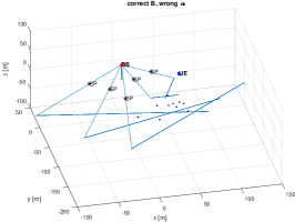
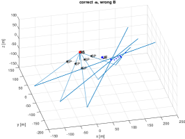
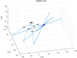
While the above reasoning was performed in a noise-free case, the noisy case can be treated by sampling:

1. Consider a hypothesis $(\alpha,B)$

2. For all $l=1,\ldots L$

   1. Given $\mathbf{z}_{l}$, generate $N_{s}\geq 1$ samples of $\bm{\phi}_{l}$ and $\rho_{l}$. For each sample $n$, generate a line segment as described above, on which $\mathbf{x}_{s,l}$ is hypothesized to lie.

   2. Given $\mathbf{z}_{l}$, generate $N_{s}\geq 1$ samples of $\bm{\phi}_{l}$, $\rho_{l}$ and $\bm{\theta}_{l}$. For each sample $n$, generate a line segment as described above, on which $\mathbf{x}$ is hypothesized to lie. We denote the segment by $\ell_{l}^{(n)}$

3. For each sample $n=1,\ldots,N_{s}$, compute the distance $d_{l,l^{\prime}}^{(n)}$ between $\ell_{l}^{(n)}$ and $\ell_{l^{\prime}}^{(n)}$ , $l\neq l^{\prime}$. At the same time, determine the unique point in 3D at minimum distance to $\ell_{l}^{(n)}$ and $\ell_{l^{\prime}}^{(n)}$. Denote this point by $\mathbf{x}_{l,l^{\prime}}^{(n)}$. Fig. 1 shows these lines for a scenario with $L=5$ (leading to 10 lines) and $N_{s}=1$. We observe that the points $\mathbf{x}_{l,l^{\prime}}^{(n)}$ are more concentrated around the UE location when the hypothesis $(\alpha,B)$ is correct.

4. Compute an error metric

   $$\mathcal{E}(\alpha,B)=\frac{2}{N_{s}(L(L-1))}\sum_{n=1}^{N_{s}}\sum_{l=1}^{L}\sum_{l^{\prime}>l}d_{l,l^{\prime}}^{(n)}$$

   and a distribution of the UE location:

   $$\bm{\mu}_{\text{UE}}(\alpha,B) =\frac{2}{N_{s}(L(L-1))}\sum_{n=1}^{N_{s}}\sum_{l=1}^{L}\sum_{l^{\prime}>l}\mathbf{x}_{l,l^{\prime}}^{(n)}$$

   $$\bm{\Sigma}_{\text{UE}}(\alpha,B) =\frac{2}{N_{s}(L(L-1))}\sum_{n=1}^{N_{s}}\sum_{l=1}^{L}\sum_{l^{\prime}>l}(\mathbf{x}_{l,l^{\prime}}^{(n)}-\bm{\mu}_{\text{UE}}(\alpha,B))(\mathbf{x}_{l,l^{\prime}}^{(n)}-\bm{\mu}_{\text{UE}}(\alpha,B))^{\text{T}},$$

   where the expectation is computed using a sample average.

The best guess for $(\alpha,B)$ is then

$$(\alpha^{*},B^{*})=\arg\min_{(\alpha,B)}\mathcal{E}(\alpha,B),$$

for which the UE position has been already computed. Finally, given the UE position distribution and the value of $(\alpha^{*},B^{*})$, it is straightforward to generate values of the SPs.

III Numerical Results

Figure 2: Surface plot of the error metric $\mathcal{E}(\alpha,B)$. The true values were $\alpha=\pi/3$ and $B=20\,\text{m}$, marked with a blue star. The estimated value $(\alpha^{*},B^{*})$ is marked with a red star.

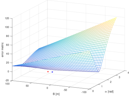
We consider a scenario with $L=5$ SPs and a measurement covariance $\bm{\Sigma}_{l}=(\text{diag}[0.1,0.01,0.01,0.01,0.01])^{2},$i.e., 10 cm TOA standard deviation and 0.01 rad AOD and AOA standard deviation. Using $N_{s}=10$ and a grid of values in the $(\alpha,B)$ space, resulting error metric $\mathcal{E}(\alpha,B)$ is shown in Fig. 2. We make a number of observations. First of all, the error metric is rather smooth and has a unique global minimum. The error function is steep along the $\alpha$ axis but broad along the $B$ axis. This is because a different value of $\alpha$ will lead to line segments pointing in many different directions, leading to a larger error value. In contrast, a different value of $B$ will lead to line segment that nearly intersect, leading to only a very small increase in the error metric. Overall, the figure indicates that a coarse search over $\alpha$for an arbitrary value of $B$, followed by a gradient descent type method can recover the global minimum. This indicates that it is easier to determine the UE rotation than it is to synchronize the user.

Figure 3: Locations of the UE and the SPs, as well as their estimates (connected with lines).

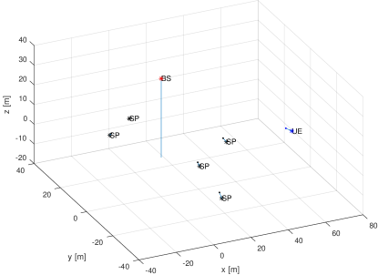
Next, after the global search is completed, we look into the quality of the positioning and the map (determining the SP locations). The result is shown in Fig. 3. We observe that while we are able to determine all the unknowns, the error in the clock bias leads to a shifting of the entire map towards the BS. Nevertheless, we have been able to provide a rough initial estimate along with a measure of uncertainty (not shown in the figure).

IV Conclusions

We have presented a simple method to initialize downlink 5G positioning in the challenging case where LOS is blocked, the position of the user is unknown, there is no a priori map information, the user has an unknown orientation, and the user and base station are not synchronized. The method is based on a geometric consistency argument, where all paths from the base station to the incidence points and to the user must intersect in a fixed location (the user’s location). Simulation results indicate that it is much easier to determine the user’s orientation that it’s clock bias. The method may have use as a pre-processor for more refined positioning, synchronization, and mapping algorithms. Complete source code is available at https://github.com/henkwymeersch/NLOSPosSynInit.

References

- [1] A. Shahmansoori, G. E. Garcia, G. Destino, G. Seco-Granados, and H. Wymeersch, “Position and orientation estimation through millimeter-wave MIMO in 5G systems,” IEEE Trans. Wireless Commun., vol. 17, pp. 1822–1835, Mar. 2018.
- [2] J. Talvitie, M. Valkama, G. Destino, and H. Wymeersch, “Novel algorithms for high-accuracy joint position and orientation estimation in 5G mmwave systems,” in IEEE Globecom Workshops, 2017.
- [3] R. Mendrzik, H. Wymeersch, and G. Bauch, “Joint localization and mapping through millimeter wave MIMO in 5G systems –extended version,” arXiv preprint arXiv:1804.04417, 2018.