Methyl cyanide (CH₃CN) and propyne (CH₃CCH) in the low mass protostar IRAS 16293–2422

Abstract

Methyl cyanide (CH₃CN) and propyne (CH₃CCH) are two molecules commonly used as gas thermometers for interstellar gas. They are detected in several astrophysical environments and in particular towards protostars. Using data of the low-mass protostar IRAS 16293–2422 obtained with the IRAM 30m single-dish telescope, we constrained the origin of these two molecules in the envelope of the source. The line shape comparison and the results of a radiative transfer analysis both indicate that the emission of CH₃CN arises from a warmer and inner region of the envelope than the CH₃CCH emission. We compare the observational results with the predictions of a gas-grain chemical model. Our model predicts a peak abundance of CH₃CCH in the gas-phase in the outer part of the envelope, at around 2000 au from the central star, which is relatively close to the emission size derived from the observations. The predicted CH₃CN abundance only rises at the radius where the grain mantle ices evaporate, with an abundance similar to the one derived from the observations.

1 Introduction

Star-forming regions are ideal places for the development of the chemical complexity in the interstellar medium. The molecules detected in these regions can be used to better understand the network of interactions between all present species that can lead to the formation of more complex molecules. All the species with 6 atoms or more and at least one atom of carbon, that are detected in the interstellar medium, are complex organic molecules (COMs, Herbst & van Dishoeck 2009). The formation of these species and their origin, either from gas-phase or dust surface reactions, is still highly debated.

In addition to their chemical interest, molecules allow astronomers to constrain the physics of the studied regions. For example, some molecules probe shocks (SO, Viti et al., 2001; Podio et al., 2015) when others can be used to constrain the density or the temperature (for instance HC₃N, Dickens et al., 2000). In particular, symmetric top molecules are good indicators of the temperature of the source. Propyne (also called methyl acetylene, CH₃CCH) and methyl cyanide (CH₃CN) belong to this category (Askne et al., 1984; Kalenskii et al., 2000). These two molecules have been detected in a lot of environments: massive young stellar objects (e.g., Fayolle et al., 2015), low-mass star-forming regions (e.g., van Dishoeck et al., 1995), photodissociation regions (e.g., Gratier et al., 2013; Guzmán et al., 2014), circumstellar envelopes of evolved stars (e.g., Agúndez et al., 2008, 2015), and even other galaxies (e.g., Mauersberger et al., 1991). Both molecules have also been detected in dense and cold cores (e.g., Vastel et al., 2014; Gratier et al., 2016), while CH₃CN was also found towards a protoplanetary disk (Öberg et al., 2015).

In this study, we focus on the study of these two complex molecules towards the solar-type protostar IRAS 16293–2422 (hereafter IRAS16293), using data obtained with the IRAM-30m telescope. This deeply embedded source, located in the $\rho$ Ophiuchi cloud, is a binary composed of source A (South-East) and source B (North-West), which are separated by about 5$\arcsec$, i.e. about 750 au at a distance of about 141 pc (Ortiz-León et al., 2017; Dzib et al., 2018). This object is at a very early stage of the star formation process (Class 0, André et al. 1993) and has been characterized by the presence of numerous complex organic molecules in the warm inner regions of the two components, where the icy grain mantles thermally desorb (Cazaux et al., 2003; Bottinelli et al., 2004; Bisschop et al., 2008; Jørgensen et al., 2011, 2012; Jørgensen et al., 2016; Kahane et al., 2013; Lykke et al., 2017; Ligterink et al., 2017). A more complete description of this source is presented in Jørgensen et al. (2016).

Using the 30m IRAM single dish antenna, we have carried out a 16 GHz spectral survey of the source. Based on these observations and using similar radiative transfer analysis, we have published, in the past, studies about CH₃SH (Majumdar et al., 2016), c-C₃HD (Majumdar et al., 2017), and HOCO⁺ (Majumdar et al., 2018). In this paper, we present a consistent analysis of CH₃CCH and CH₃CN. This paper is organized as follows. In Section 2, we present the data, their analysis, and the observational results. Section 3 includes a description of the chemical model and its results in comparison with the observations. Last, we conclude in Section 4.

2 Observations and data reduction

2.1 Observations

Observations were performed using the IRAM 30m telescope from August 18 to 23, 2015 in average summer conditions (a median value of 4-6mm water vapor). The EMIR heterodyne 3mm receiver tuned at a frequency of 89.98 GHz was used in the Lower Inner sideband and paired with the Fourier Transform Spectrometer in its 195 kHz resolution mode. The observed spectrum is composed of two approximately 8 GHz regions centered respectively on 88.41 and 104.06 GHz. The typical angular resolution is 24-28^′′. The wobbler switching mode with a throw of 90" and a period of 2 seconds was used to make observations centered at the position $\alpha$2000 = 16h32m22.75s, $\delta$2000 = -24^o28’34.2" , midway between sources A and B of IRAS16293. This throw ensures a flat baseline even for observations at low elevation and in summer conditions. Moreover, at the beginning of each run and after sunset, the nearby planet Saturn was used for focus. Pointing was checked hourly on nearby quasars with a pointing correction less than a third of the beam.

2.2 Line properties of CH₃CN and CH₃CCH

Table 1: Spectroscopic parameters and observed line properties.

Molecules	QNs	Frequency	Ai,j	Eup	gup	Tpeak	$\sigma$	Area	$\varv_{\rm LSR}$	FWHM
	$J_{K}\rightarrow J^{\prime}_{K}$	(MHz)	(s-1)	(K)		(mK)	(mK)	(K km s-1)	(km s-1)	(km s-1)
CH3CN	$5_{4}\rightarrow 4_{4}$	91958.726	$2.28\times 10^{-5}$	127.5	22	36.2	1.93	0.312$\pm$0.005	3.0$\pm$0.3	8.3$\pm$0.2
CH3CN	$5_{3}\rightarrow 4_{3}$	91971.130	$4.05\times 10^{-5}$	77.5	44	91.2	3.07	0.68$\pm$0.01	2.95$\pm$0.05	7.0$\pm$0.1
CH3CN	$5_{2}\rightarrow 4_{2}$	91979.994	$5.32\times 10^{-5}$	41.8	22	86.5	2.86	0.553$\pm$0.008	3.00$\pm$0.05	6.0$\pm$0.1
CH3CN	$5_{1}\rightarrow 4_{1}$	91985.314	$6.08\times 10^{-5}$	20.4	22	113	2.13	0.679$\pm$0.008	3.40$\pm$0.03	5.60$\pm$0.07
CH3CN	$5_{0}\rightarrow 4_{0}$	91987.088	$6.33\times 10^{-5}$	13.2	22	115	2.09	0.672$\pm$0.001	2.92$\pm$0.01	5.49$\pm$0.05
CH3CCH	$5_{4}\rightarrow 4_{4}$	85431.174	$7.30\times 10^{-7}$	127.9	22	$<7.32$	2.44	-	-	-
CH3CCH	$5_{3}\rightarrow 4_{3}$	85442.601	$1.30\times 10^{-6}$	77.3	44	2.63	2.51	0.090$\pm$0.006	3.5$\pm$0.1	3.2$\pm$0.3
CH3CCH	$5_{2}\rightarrow 4_{2}$	85450.766	$1.70\times 10^{-6}$	41.2	22	70.9	2.11	0.145$\pm$0.004	3.62$\pm$0.02	1.92$\pm$0.06
CH3CCH	$5_{1}\rightarrow 4_{1}$	85455.667	$1.95\times 10^{-6}$	19.5	22	207	2.83	0.398$\pm$0.005	3.62$\pm$0.01	1.78$\pm$0.03
CH3CCH	$5_{0}\rightarrow 4_{0}$	85457.300	$2.03\times 10^{-6}$	12.3	22	267	2.72	0.497$\pm$0.004	3.691$\pm$0.008	1.75$\pm$0.02
CH3CCH	$6_{5}\rightarrow 5_{5}$	102499.019	$1.09\times 10^{-6}$	197.8	26	$<7.38$	2.46	-	-	-
CH3CCH	$6_{4}\rightarrow 5_{4}$	102516.637	$1.98\times 10^{-6}$	132.8	26	$<6.48$	2.16	-	-	-
CH3CCH	$6_{3}\rightarrow 5_{3}$	102530.348	$2.67\times 10^{-6}$	82.3	52	43.2	1.29	0.13$\pm$0.03	3.7$\pm$0.3	2.8$\pm$0.7
CH3CCH	$6_{2}\rightarrow 5_{2}$	102540.145	$3.16\times 10^{-6}$	46.1	26	98.5	7.16	0.2$\pm$0.1	3.8$\pm$0.6	2.4$\pm$0.8
CH3CCH	$6_{1}\rightarrow 5_{1}$	102546.024	$3.46\times 10^{-6}$	24.5	26	218	5.85	0.6$\pm$0.1	3.8$\pm$0.1	2.1$\pm$0.4
CH3CCH	$6_{0}\rightarrow 5_{0}$	102547.984	$3.56\times 10^{-6}$	17.2	26	262	4.96	0.71$\pm$0.08	3.8$\pm$0.1	2.1$\pm$0.3

Notes: QNs: quantum numbers, Frequency: transition rest frequency, A_i,j: Einstein coefficient of spontaneous emission of a photon by transition from level $j$ to level $i$, E_up: energy of the upper level, g_up: statistical degeneracy of the upper level, T_peak: peak observed main beam temperature, $\sigma$: observed noise, Area: observed integrated intensity, $\varv_{\rm LSR}$: observed doppler velocity shift, FWHM: observed line full width at half maximum.

Table 2: Prior distribution functions for the parameters used in the Bayesian approach.

Name	Parameter	Distribution	Comment
Molecular column density	$\log$ N (cm-2)	Uniform(8,22)
Excitation temperature	Tex (K)	Normal(40,40)	limited to T>2.73K
Radius of the emission	$\log$ R (au)	Normal($\log(R(T))$,0.01)	$R(T)$ is the relationship from Crimier et al. 2010
Doppler shift	$\varv_{LSR}$ (km s-1)	Uniform(2.8,4.8)
FWHM of the emission	$\Delta\varv$ (km s-1)	Normal(5,5)
Additional noise	$\sigma_{\rm add}$ (mK)	Normal(0,1)

Notes: Uniform($x_{l}$,$x_{u}$) is the uniform random distribution that can take values between $x_{l}$ and $x_{u}$, Normal($\mu$,$\sigma$) is the normal (gaussian) random distribution with mean $\mu$ and standard deviation $\sigma$.

Table 3: Point estimates of the posterior distribution function corresponding to the median and one sigma uncertainty for CH₃CN and CH₃CCH.

Parameter	CH3CCH	CH3CN
$\log$ N (cm-2)	14.73$\pm$0.03	16.14$\pm$ 0.05
Tex (K)	25$\pm$1	75$\pm$2
$\varv_{LSR}$ (km s-1)	3.79$\pm$0.01	3.18$\pm$0.06
$\theta(^{\prime\prime})$	11.7$\pm$0.5	1.19$\pm$0.04
$\Delta\varv$ (km s-1)	1.99$\pm$0.02	5.1$\pm$0.1
$\log[X]^{a}$	-9.63$\pm$0.03	-8.10$\pm$0.06
$\log N_{H_{tot}}$b	24.36$\pm$0.002	24.26$\pm$0.03

Notes: $\theta(^{\prime\prime})$ is the source size, ${}^{a}[X]=N_{x}/N_{H_{tot}}$, ^b $N_{H_{tot}}$ is the total hydrogen nucleon density.

In Table 1, we provide some line properties. The spectroscopic data, extracted from the CDMS database (Müller et al., 2005), are from Müller et al. (2015) for CH₃CN and Cazzoli & Puzzarini (2008) for CH₃CCH. We used the CLASS software, from the GILDAS package, to reduce and analyse the data. Gaussian fits were made to the detected lines following a local low (typically 0th) order polynomial baseline subtraction. Table 1 shows the results of these fits for the 5 observed lines of CH₃CN and 8 observed lines of CH₃CCH. Three CH₃CCH observed lines are below the detection level and we report the 3$\sigma$ detection limit in Table 1. For CH₃CCH, the mean LSR velocity is 3.7 km s^-1 and the mean FWHM is 2.3 km s^-1 while for CH₃CN, the LSR velocity is 3.1 km s^-1 and the mean FWHM is 6.5 km s^-1.

2.3 CH₃CN and CH₃CCH radiative transfer modeling

We use a Bayesian approach similar to the one presented in Majumdar et al. (2016) to recover the distribution of parameters. The radiative transfer modeling is carried out assuming Local Thermal Equilibrium. In addition to the fitting uncertainties, we allowed for a 10% calibration error. The modelled line profiles are computed as a function of the molecule column density, excitation temperature, line width, systemic velocity, and source size (described by a two dimensional circular Gaussian source profile centered in the telescope beam). The line shapes are computed assuming a Gaussian opacity profile as a function of frequency. In our computation, we have used the relation between the source size and the temperature profile determined by Crimier et al. (2010) (see their Fig. 7). Crimier et al. (2010) have determined the density and temperature profiles (at large spatial scale) of the IRAS16293 protostellar envelope using continuum data (single dish and interferometric, from millimeter to MIR) and ISO water observations. They showed that the densities remain higher than $10^{6}$ cm^-3 even at a distance of 2000 au from the two central objects. This is higher than the typical critical densities for the observed transitions of CH₃CN that can be computed using the available collisional coefficients from Green (1986), that cover a range between $8\times 10^{4}$ cm^-3 and $5\times 10^{5}$ cm^-3 at 60K. The LTE approximation should remain valid for our study. Collisional coefficients for CH₃CCH are not known.

The sampling of the posterior distribution function was carried out using the No-U-Turns (NUTS) Hamiltonian Monte Carlo sampler implemented in the Stan Probabilistic Programming Language (Carpenter et al., 2017) with the Pystan interface. Four independent chains were run for 4000 iterations, discarding the first half for burn-in and the adaptation of the Hamiltonian Monte Carlo NUTS parameters. Convergence was checked by computing the Gelman-Rubin $\hat{R}$ test (Gelman & Rubin, 1992) ensuring that the values were below 1.01 for all parameters. The properties of the prior distributions are given in Table 2.

Figures 1 and 2 show the 1D and 2D histograms of the posterior probability distribution function and the comparison of the observations with the distribution of computed intensities corresponding to the posterior distribution of parameters. The summary of the point estimates for both molecules is presented in Table 3. Integrating the density power law from Crimier et al. (2010) up to the source size emission (itself determined by comparing the excitation temperature of the molecules to the temperature profile from Crimier et al.) derived by the Bayesian method allows us to get an estimate of the H₂ column density of the emitting zone. The derived H₂ column densities are $2.3\times 10^{24}$ cm^-2 for CH₃CCH and $1.8\times 10^{24}$ cm^-2 for CH₃CN. The observed and modelled spectra for the four lines of CH₃CN and the 8 detected lines of CH₃CCH are displayed in Figs. 3 and 4. The features not fitted by the model in Fig. 3 probably arise from second order effects of radiative transfer (i.e. self absorption) through the colder envelope that cannot be modelled by our 0D approach.

2.4 Results

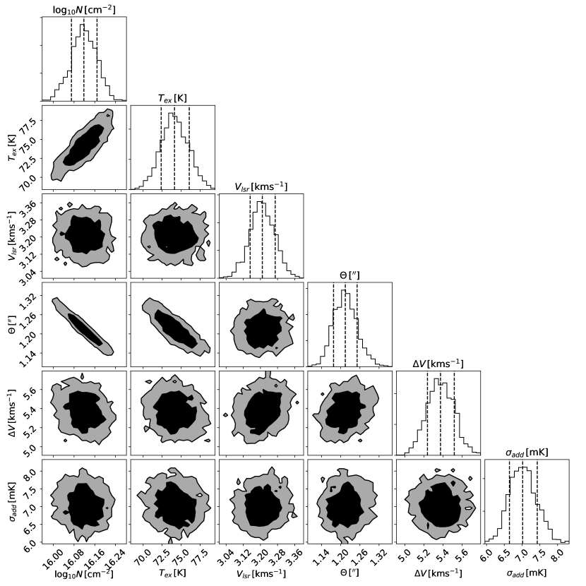
Figure 1: One-dimensional and two-dimensional (i.e. contour) histograms of the posterior distribution of parameters for CH₃CN. Contours contain 68% and 95% of samples, respectively. Vertical dashed lines correspond to 16%, 50%, and 84% of the samples.

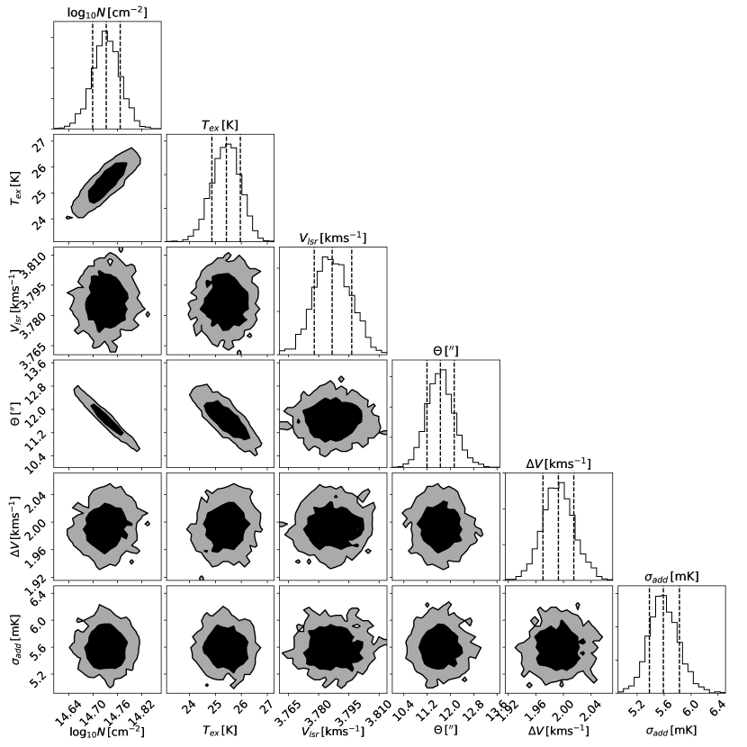
Figure 2: Same as Fig. 1 but for CH₃CCH.

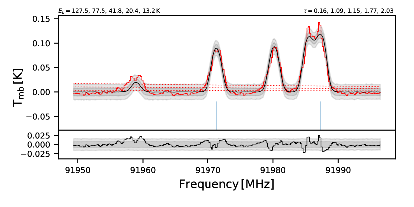
Figure 3: Upper panel: observed (red) and modelled spectra for CH₃CN. The modelled spectra are represented by the median of the distribution of models (solid line) along with the associated $1\sigma$ (dark grey) and $2\sigma$ (light grey) uncertainties, the thin vertical blue lines are the frequencies of the fitted lines, the red dotted lines correspond to the $1\sigma$, $3\sigma$, and $5\sigma$ noise level. Lower panel: distribution of the residuals plotted as the median (solid line) along with the associated $1\sigma$ (dark grey) and $2\sigma$ (light grey) uncertainties. Top left: values of the upper energy levels of the lines from left to right, top right: median values of the inferred opacities for the lines.

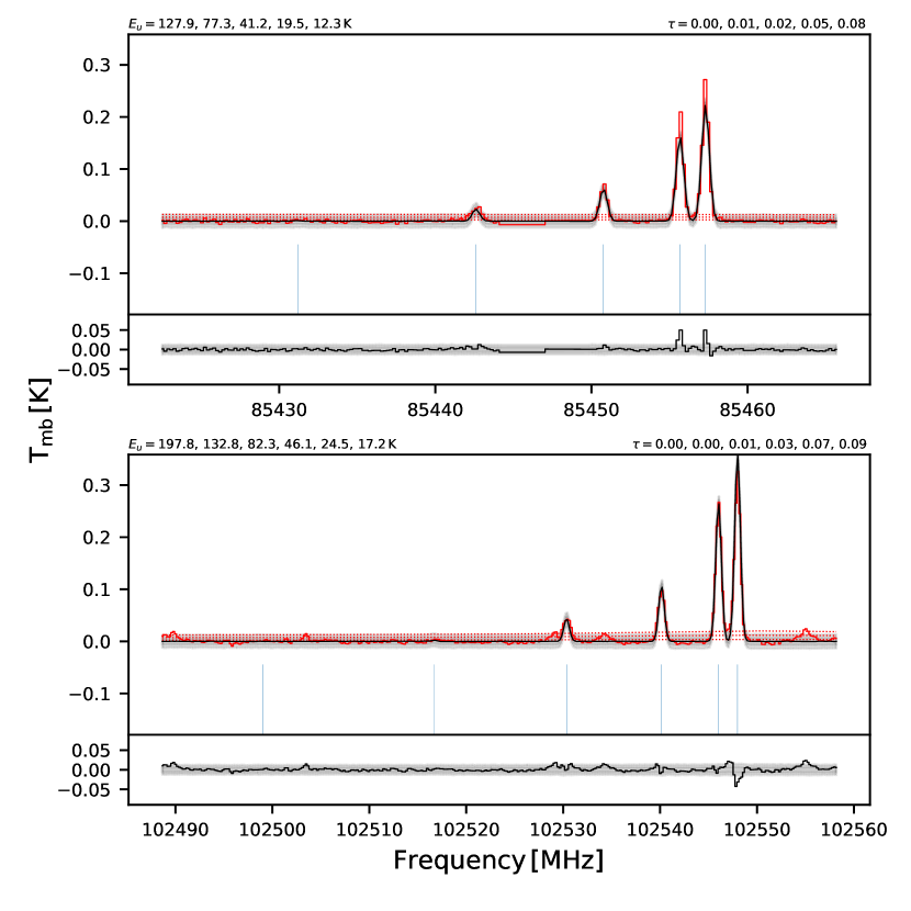
Figure 4: Same as Fig. 3 but for CH₃CCH.

According to the classification proposed by Caux et al. (2011), both species are of kinematic type IV, meaning that their emission probably comes from both components of the source (A and B), and the common envelope. The rest velocities and the line widths of the CH₃CCH lines are similar to those of molecules probing the cold envelope of the protostellar system (v_LSR $\sim$3.9 km s^-1 and FWHM$\sim$2 km s^-1, Caux et al., 2011). The CH₃CN lines, on the contrary, present larger widths $>$ 5.5 km s^-1. The computed excitation temperatures are different for these two molecules and much higher for CH₃CN (75 K) as compared to CH₃CCH (25 K). These results seem to indicate that the CH₃CN emission comes from a warmer region, probably associated with the hot corino(s), while the CH₃CCH emission comes from the colder outer envelope. Based on the excitation temperatures and the radial temperature profile used, the CH₃CN emission would come from about 170 au from the central star whereas CH₃CCH would come from about 1700 au (assuming the most recent distance of the source, i.e. 141 pc). Integrating the total hydrogen nucleon density column density from Crimier et al. (2010) within these radii, we obtain abundances of $2\times 10^{-10}$ for CH₃CCH and $8\times 10^{-9}$ for CH₃CN (with respect to the total hydrogen nucleon density). In addition, the structure determined by Crimier et al. (2010) has to be taken with caution as the authors assumed a distance of 120 pc for the source while this value has recently been revisited to a larger one (i.e. 141 pc, Ortiz-León et al., 2017; Dzib et al., 2018).
The structure of IRAS16293 used in the paper is assumed to be spherical, although it is a binary source with a complex structure in the inner regions (Jørgensen et al., 2016; Jacobsen et al., 2018). The dust properties are also very uncertain in these regions. This has consequences on the derived abundance with respect to H₂. If the molecular emission comes from large scales, the abundance with respect to H₂ should be relatively well constrained while the abundances in the inner regions (within a few arcsec) would be more uncertain. The absolute abundance of CH₃CCH should consequently be better constrained than the one of CH₃CN. If the emission of the molecule is only at a certain radius of the envelope, the derived abundances should be considered as upper limits. Recent ALMA analysis of CH₃CN show that this molecule in indeed emitting towards both protostellar sources and does not show any significant difference between the two sources. Calcutt et al. (2018b) obtain a very similar column density (within a factor 2) for the two components. If we correct the column densities determined in Calcutt et al. (2018b) by the source size constrained in this paper, the column density we obtain is in fact the average of the column densities of the two sources, which confirms that our analysis is correct. For the CH₃CCH molecule, since the emission is much more extended, the values derived here should be less biased by the multiplicity of the source.

3 Comparison with chemical models

3.1 Model description

To simulate the chemistry in the envelope of IRAS16293, the 3-phase Nautilus gas-grain code has been used (Ruaud et al., 2016). This numerical model computes the gas and ice composition as a function of time by solving a set of differential equations, which relate the species abundances to the chemical rates. In addition to the gas-phase reactions (see Wakelam et al., 2015), interactions between the gas-phase species and the grain surfaces are included: physisorption of gas-phase species onto the grains and thermal and non thermal desorption. For the non thermal desorption, cosmic-ray induced desorption (Hasegawa & Herbst, 1993), photodesorption (see Ruaud et al., 2016), and chemical desorption (Garrod et al., 2007) are included. Reactions at the surface of the grains follow the Langmuir-Hinshelwood theory. All the parameters for the surface chemistry are the same as in Ruaud et al. (2016) while the gas and surface chemical networks are the same as in Vidal et al. (2017).

Using this code, the chemistry is then computed in cells of material falling into the centre of the protostar. The physical parameters (temperatures, densities, and visual extinctions) are the results of radiation hydrodynamical simulations from Masunaga & Inutsuka (2000). This structure has already been used in several previous studies of this source (Aikawa et al., 2008, 2012; Wakelam et al., 2014; Bottinelli et al., 2014; Majumdar et al., 2016; Majumdar et al., 2017). The time dependent density and temperature profiles are shown in Fig. 2 of Aikawa et al. (2008). As already discussed in Wakelam et al. (2014), the physical structure at the end of the hydrodynamical simulations is similar to the temperature and density gradients derived by Crimier et al. (2010) from the observations for IRAS16293 (see Fig. 1 of Wakelam et al., 2014, for a comparison). The density structure is however approximately ten times smaller than the observed one. As in previous studies, we then multiply all the densities of the physical model (at all times and all radii) by a factor of ten to be closer to the observations. The physical model is then not self-consistent anymore. However, in the absence of a time-dependent physical model reproducing the exact observed structure, we decided to use this one because the effect of the dynamics has a major impact on the chemical structure of the envelope (Vidal & Wakelam, 2018). See Wakelam et al. (2014) for a complete discussion on this point.

We use as initial abundances for this dynamical model the output of a dark cloud chemical simulation. The physical parameters of this initial simulation are: a gas and dust temperature of 10 K, a total hydrogen nucleon density of $2\times 10^{4}$ cm^-3, a cosmic-ray ionization rate of $1.3\times 10^{-17}$ s^-1, and a visual extinction of 15 mag. The set of elemental abundances we used is summarized in Table 4. We start with all species in their atomic or ionized form, with the exception of hydrogen, which is assumed to be entirely in its molecular form. Vidal et al. (2017) showed that the Nautilus chemical model does not require additional depletion of sulphur from its cosmic value in order to reproduce dark clouds observations, we therefore use it as the initial sulphur abundance. The final chemical composition obtained for a cloud age of 10⁶ yrs is then used as initial conditions for the collapsing source. The choice of the initial cloud age is always a difficult one as the chemical modeling result may depend on this. With the dynamical physical structure used here, Vidal & Wakelam (2018) however showed that the model predictions do not depend much on the cloud age. We tested with a younger cloud of $10^{5}$ yrs and this is indeed the case for CH₃CCH and CH₃CN.

After running the chemical model for the different infalling cells of material, we reconstruct the final chemical composition of the protostellar envelope in 1D, and this is what is shown in the next section.

Table 4: Elemental abundances used for the dark cloud run. *$a(b)$ stands for $a\times 10^{b}$

Element	$n_{i}/n_{H}$*	References
H2	0.5
He	0.09	1
N	6.2(-5)	2
O	2.4(-4)	3
C+	1.7(-4)	2
S+	1.5(-5)	2
Si+	8.0(-9)	4
Fe+	3.0(-9)	4
Na+	2.0(-9)	4
Mg+	7.0(-9)	4
P+	2.0(-10)	4
Cl+	1.0(-9)	4
F	6.7(-9)	5

(1) Wakelam & Herbst (2008), (2) Jenkins (2009), (3) Hincelin et al. (2011), (4) Low-metal abundances from Graedel et al. (1982), (5) Depleted value from Neufeld et al. (2005)

3.2 Chemical model results

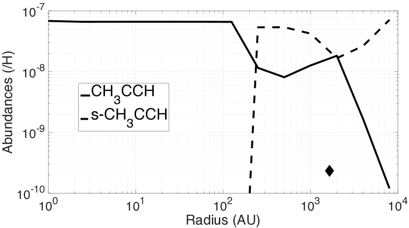
Figure 5: Solid (dotted line) and gas-phase (solid line) CH₃CCH abundances predicted by the chemical model at the end of the simulations as a function of radius to the centre of the protostar. The diamond represents the observed abundance at the expected location.

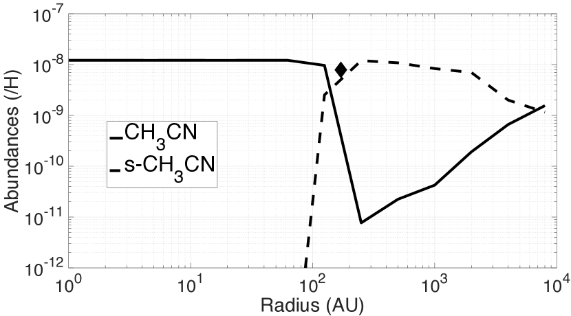
Figure 6: Solid (dotted line) and gas-phase (solid line) CH₃CN abundances predicted by the chemical model at the end of the simulations as a function of radius to the centre of the protostar. The diamond represents the observed abundance at the expected location.

Figures 5 and 6 show solid and gas-phase abundances of CH₃CCH and CH₃CN respectively computed by the chemical model at the end of the protostellar simulations (i.e. at $3.43\times 10^{5}$ yr after the beginning of the collapse). For both molecules, the solid phase abundance at radii larger than 200 au is higher than the gas-phase one showing that both molecules are probably efficiently produced on the grains at low temperature. Indeed CH₃CCH is formed on the grain surface through successive hydrogenation of physisorbed C₃ (Hickson et al., 2016), by:

$$\text{C${}_{3}$}\xrightarrow{\text{H}}\text{c-C${}_{3}$H}\xrightarrow{\text{H}}\text{c-C${}_{3}$H${}_{2}$}\xrightarrow{\text{H}}\text{CH${}_{2}$CCH}\xrightarrow{\text{H}}\text{CH${}_{3}$CCH}$$ (1)

In this model, the large abundance of C₃ is due to various efficient production pathways in the gas-phase associated with an absence of efficient destruction reactions as C₃ does not react quickly with H, N, C or O atoms (see Hickson et al., 2016).

CH₃CN is also efficiently formed on the grain surface through the hydrogenation of adsorbed H₂CCN, which is originally formed in the gas phase by:

$$\text{CN}+\text{CH${}_{3}$}\to\text{H}+\text{H${}_{2}$CCN}$$ (2)

For both species, their solid-state abundances drop sharply around 200 au because they are evaporated from the surfaces as the cells of material are moving inward. The binding energies used in the model are 3800 K for CH₃CCH and 4680 K for CH₃CN (Wakelam et al., 2017) so that the evaporation temperature is slightly higher for CH₃CN and the molecule desorbs closer to the protostars. The evaporation radius depends obviously on the assumed binding energies. Recent experimental results on the CH₃CN binding energies on water ices by Bertin et al. (2017) gave a mean binding energy of 6150 K, i.e. much larger than what we have used for this work. Using such value would put the evaporation radius of this molecule closer to the central star but would not change the abundance values as it would not change much its diffusion on the surface. This conclusion would also apply to CH₃CCH, i.e. a change of binding energy for this species would just change the evaporation radius. It should however be noted that the new binding energy of CH₃CN should be taken with great care as noted in Bertin et al. (2017) because of the co-desorption of water with CH₃CN during the experiment.
The predicted gas-phase abundance of CH₃CCH in the outer envelope is quite high compared to the one of CH₃CN. Indeed, in the cold envelope (T < 20 K), CH₃CCH is also efficiently formed in the gas-phase from the hydrocarbons C₂H₄ and C₃H₅ produced in the parent cold cloud via the following reactions:

$$\text{C${}_{2}$H${}_{4}$}+\text{CH} \to \text{H}+\text{CH${}_{3}$CCH}$$ (3)

$$\text{C${}_{3}$H${}_{5}$}+\text{H} \to \text{H${}_{2}$}+\text{CH${}_{3}$CCH}$$ (4)

C₂H₄ is formed in the gas phase through the CH + CH₄ reaction and on grains through the hydrogenation of C₂H₂, which is formed in the gas-phase. C₃H₅ is mainly formed on grains through the hydrogenation of C₃. Although less efficient, the gas-phase production of CH₃CN is effected through the HCN + CH${}_{3}^{+}$ $\rightarrow$ CH₃CNH⁺ + h$\nu$ radiative association followed by the dissociative recombination of CH₃CNH⁺.

Going inward into the protostellar envelope to regions of higher density, the gas-phase formation of CH₃CCH is overcome by adsorption onto grain surface, explaining its abundance decrease between 2000 and 500 au. The small fraction of CH₃CN that chemically desorbs in the gas phase is preferentially consumed through several ion-neutral reactions involving H${}_{3}^{+}$, HCO⁺, He⁺ and C⁺.

4 Discussions and conclusions

Figures 5 and 6 also display the observed abundances for each species (diamonds). For both species, the comparison between the modelled and observed abundances are based on the assumption that the H₂ column density has been correctly estimated for the emission region of each species.With that in mind, the model overestimates the gas-phase abundance of CH₃CCH by about two orders of magnitude. However, interestingly, the observed abundance seems to be located at the same radius as the modelled peak abundance. Since we use single dish observations, the observed spectra are very likely not sensitive to the innermost emission of the molecule (inside 200 au, see Majumdar et al., 2016, for a discussion on this effect), where the species abundance may be quite large as predicted by the model. Dividing the observed molecular column density by the integrated H₂ column density may bias the abundance towards smaller values. Moreover, the overestimation of CH₃CCH may be due to the fact that, in the model, we consider a barrier for the O + C₃ reaction (Woon & Herbst, 1996) leading to a very large C₃ abundance in the gas phase and then a large CH₃CCH abundance on grains. The overestimation of CH₃CCH may be an indication that the O + C₃ reaction is in fact efficient at low temperature due to tunnelling similarly to the reaction O + C₃H₆ (Sabbah et al., 2007). For CH₃CN, the observed abundance could fit very well with that expected for the evaporated region.

Using JCMT observations, Schöier et al. (2002) have determined the abundance of these two molecules on the same source but with a different radiative transfer model and different physical properties of the source. The analysis of the observed emission was done with a "jump" model assuming a smaller constant abundance of the species in the outer part and a higher one inside 150 au where the temperature is larger than 90 K. Using this model with the observed higher frequency transitions (as compared to ours), the authors determined an inner region abundance of $7.5\times 10^{-9}$ for CH₃CN and $3.5\times 10^{-8}$ for CH₃CCH while they only had upper limits (of $8\times 10^{-11}$ for CH₃CN and $1.5\times 10^{-9}$ for CH₃CCH) for the outer part. Our chemical model predicts abundances in the outer regions that are not flat for both molecules; in particular for CH₃CN. Our predicted abundances for the inner regions for both molecules are very close to the ones determined by Schöier et al. (2002).

Last, it is important to keep in mind that IRAS16293 is a binary system with both components inside the same observational beam for single dish observations. Variation of the chemical composition between the two binary components is currently investigated in the framework of the ALMA-PILS survey (Jørgensen et al., 2016). Although CH₃CN shows similar column densities towards the two components, some significant variations are observed for other species such as CH₃NC (Calcutt et al., 2018b) and C₂H₃CN (Calcutt et al., 2018a), possibly due to differences in their physical conditions or evolutionary stages.

References

- Agúndez et al. (2008) Agúndez M., Fonfría J. P., Cernicharo J., Pardo J. R., Guélin M., 2008, A&A, 479, 493
- Agúndez et al. (2015) Agúndez M., Cernicharo J., Quintana-Lacaci G., Velilla Prieto L., Castro-Carrizo A., Marcelino N., Guélin M., 2015, ApJ, 814, 143
- Aikawa et al. (2008) Aikawa Y., Wakelam V., Garrod R. T., Herbst E., 2008, ApJ, 674, 984
- Aikawa et al. (2012) Aikawa Y., Wakelam V., Hersant F., Garrod R. T., Herbst E., 2012, ApJ, 760, 40
- André et al. (1993) André P., Ward-Thompson D., Barsony M., 1993, ApJ, 406, 122
- Askne et al. (1984) Askne J., Hoglund B., Hjalmarson A., Irvine W. M., 1984, A&A, 130, 311
- Bertin et al. (2017) Bertin M., et al., 2017, A&A, 598, A18
- Bisschop et al. (2008) Bisschop S. E., Jørgensen J. K., Bourke T. L., Bottinelli S., van Dishoeck E. F., 2008, A&A, 488, 959
- Bottinelli et al. (2004) Bottinelli S., et al., 2004, ApJ, 617, L69
- Bottinelli et al. (2014) Bottinelli S., Wakelam V., Caux E., Vastel C., Aikawa Y., Ceccarelli C., 2014, MNRAS, 441, 1964
- Calcutt et al. (2018a) Calcutt H., et al., 2018a, preprint, (arXiv:1807.02909)
- Calcutt et al. (2018b) Calcutt H., et al., 2018b, A&A, 616, A90
- Carpenter et al. (2017) Carpenter B., et al., 2017, Journal of Statistical Software, Articles, 76, 1
- Caux et al. (2011) Caux E., et al., 2011, A&A, 532, A23
- Cazaux et al. (2003) Cazaux S., Tielens A. G. G. M., Ceccarelli C., Castets A., Wakelam V., Caux E., Parise B., Teyssier D., 2003, ApJ, 593, L51
- Cazzoli & Puzzarini (2008) Cazzoli G., Puzzarini C., 2008, A&A, 487, 1197
- Crimier et al. (2010) Crimier N., Ceccarelli C., Maret S., Bottinelli S., Caux E., Kahane C., Lis D. C., Olofsson J., 2010, A&A, 519, A65
- Dickens et al. (2000) Dickens J. E., Irvine W. M., Snell R. L., Bergin E. A., Schloerb F. P., Pratap P., Miralles M. P., 2000, ApJ, 542, 870
- Dzib et al. (2018) Dzib S. A., et al., 2018, preprint, (arXiv:1802.03234)
- Fayolle et al. (2015) Fayolle E. C., Öberg K. I., Garrod R. T., van Dishoeck E. F., Bisschop S. E., 2015, A&A, 576, A45
- Garrod et al. (2007) Garrod R. T., Wakelam V., Herbst E., 2007, A&A, 467, 1103
- Gelman & Rubin (1992) Gelman A., Rubin D., 1992, Statistical Science, 7, 457
- Graedel et al. (1982) Graedel T. E., Langer W. D., Frerking M. A., 1982, ApJS, 48, 321
- Gratier et al. (2013) Gratier P., Pety J., Guzmán V., Gerin M., Goicoechea J. R., Roueff E., Faure A., 2013, A&A, 557, A101
- Gratier et al. (2016) Gratier P., Majumdar L., Ohishi M., Roueff E., Loison J. C., Hickson K. M., Wakelam V., 2016, ApJS, 225, 25
- Green (1986) Green S., 1986, ApJ, 309, 331
- Guzmán et al. (2014) Guzmán V. V., Pety J., Gratier P., Goicoechea J. R., Gerin M., Roueff E., Le Petit F., Le Bourlot J., 2014, Faraday Discussions, 168, 103
- Hasegawa & Herbst (1993) Hasegawa T. I., Herbst E., 1993, MNRAS, 261, 83
- Herbst & van Dishoeck (2009) Herbst E., van Dishoeck E. F., 2009, ARA&A, 47, 427
- Hickson et al. (2016) Hickson K. M., Wakelam V., Loison J.-C., 2016, Molecular Astrophysics, 3, 1
- Hincelin et al. (2011) Hincelin U., Wakelam V., Hersant F., Guilloteau S., Loison J. C., Honvault P., Troe J., 2011, A&A, 530, A61
- Jacobsen et al. (2018) Jacobsen S. K., et al., 2018, A&A, 612, A72
- Jenkins (2009) Jenkins E. B., 2009, ApJ, 700, 1299
- Jørgensen et al. (2011) Jørgensen J. K., Bourke T. L., Nguyen Luong Q., Takakuwa S., 2011, A&A, 534, A100
- Jørgensen et al. (2012) Jørgensen J. K., Favre C., Bisschop S. E., Bourke T. L., van Dishoeck E. F., Schmalzl M., 2012, ApJ, 757, L4
- Jørgensen et al. (2016) Jørgensen J. K., et al., 2016, A&A, 595, A117
- Kahane et al. (2013) Kahane C., Ceccarelli C., Faure A., Caux E., 2013, ApJ, 763, L38
- Kalenskii et al. (2000) Kalenskii S. V., Promislov V. G., Alakoz A., Winnberg A. V., Johansson L. E. B., 2000, A&A, 354, 1036
- Ligterink et al. (2017) Ligterink N. F. W., et al., 2017, MNRAS, 469, 2219
- Lykke et al. (2017) Lykke J. M., et al., 2017, A&A, 597, A53
- Majumdar et al. (2016) Majumdar L., Gratier P., Vidal T., Wakelam V., Loison J.-C., Hickson K. M., Caux E., 2016, MNRAS, 458, 1859
- Majumdar et al. (2017) Majumdar L., Gratier P., Andron I., Wakelam V., Caux E., 2017, MNRAS, 467, 3525
- Majumdar et al. (2018) Majumdar L., Gratier P., Wakelam V., Caux E., Willacy K., Ressler M. E., 2018, MNRAS, 477, 525
- Masunaga & Inutsuka (2000) Masunaga H., Inutsuka S.-i., 2000, ApJ, 531, 350
- Mauersberger et al. (1991) Mauersberger R., Henkel C., Walmsley C. M., Sage L. J., Wiklind T., 1991, A&A, 247, 307
- Müller et al. (2005) Müller H. S. P., Schlöder F., Stutzki J., Winnewisser G., 2005, Journal of Molecular Structure, 742, 215
- Müller et al. (2015) Müller H. S. P., et al., 2015, Journal of Molecular Spectroscopy, 312, 22
- Neufeld et al. (2005) Neufeld D. A., Wolfire M. G., Schilke P., 2005, ApJ, 628, 260
- Öberg et al. (2015) Öberg K. I., Guzmán V. V., Furuya K., Qi C., Aikawa Y., Andrews S. M., Loomis R., Wilner D. J., 2015, Nature, 520, 198
- Ortiz-León et al. (2017) Ortiz-León G. N., et al., 2017, ApJ, 834, 141
- Podio et al. (2015) Podio L., et al., 2015, A&A, 581, A85
- Ruaud et al. (2016) Ruaud M., Wakelam V., Hersant F., 2016, MNRAS, 459, 3756
- Sabbah et al. (2007) Sabbah H., Biennier L., Sims I. R., Georgievskii Y., Klippenstein S. J., Smith I. W. M., 2007, Science, 317, 102
- Schöier et al. (2002) Schöier F. L., Jørgensen J. K., van Dishoeck E. F., Blake G. A., 2002, A&A, 390, 1001
- Vastel et al. (2014) Vastel C., Ceccarelli C., Lefloch B., Bachiller R., 2014, ApJ, 795, L2
- Vidal & Wakelam (2018) Vidal T. H. G., Wakelam V., 2018, MNRAS, 474, 5575
- Vidal et al. (2017) Vidal T. H. G., Loison J.-C., Jaziri A. Y., Ruaud M., Gratier P., Wakelam V., 2017, MNRAS, 469, 435
- Viti et al. (2001) Viti S., Caselli P., Hartquist T. W., Williams D. A., 2001, A&A, 370, 1017
- Wakelam & Herbst (2008) Wakelam V., Herbst E., 2008, ApJ, 680, 371
- Wakelam et al. (2014) Wakelam V., Vastel C., Aikawa Y., Coutens A., Bottinelli S., Caux E., 2014, MNRAS, 445, 2854
- Wakelam et al. (2015) Wakelam V., et al., 2015, ApJS, 217, 20
- Wakelam et al. (2017) Wakelam V., Loison J.-C., Mereau R., Ruaud M., 2017, Molecular Astrophysics, 6, 22
- Woon & Herbst (1996) Woon D. E., Herbst E., 1996, ApJ, 465, 795
- van Dishoeck et al. (1995) van Dishoeck E. F., Blake G. A., Jansen D. J., Groesbeck T. D., 1995, ApJ, 447, 760