An Empirical Study of Example Forgetting during Deep Neural Network Learning
Abstract
Inspired by the phenomenon of catastrophic forgetting, we investigate the learning dynamics of neural networks as they train on single classification tasks. Our goal is to understand whether a related phenomenon occurs when data does not undergo a clear distributional shift. We define a “forgetting event” to have occurred when an individual training example transitions from being classified correctly to incorrectly over the course of learning. Across several benchmark data sets, we find that: (i) certain examples are forgotten with high frequency, and some not at all; (ii) a data set’s (un)forgettable examples generalize across neural architectures; and (iii) based on forgetting dynamics, a significant fraction of examples can be omitted from the training data set while still maintaining state-of-the-art generalization performance.
Code available at https://github.com/mtoneva/example_forgetting
1 Introduction
Many machine learning models, in particular neural networks, cannot perform continual learning. They have a tendency to forget previously learnt information when trained on new tasks, a phenomenon usually called catastrophic forgetting (Kirkpatrick et al., 2017; Ritter et al., 2018). One of the hypothesized causes of catastrophic forgetting in neural networks is the shift in the input distribution across different tasks—e.g., a lack of common factors or structure in the inputs of different tasks might lead standard optimization techniques to converge to radically different solutions each time a new task is presented. In this paper, we draw inspiration from this phenomenon and investigate the extent to which a related forgetting process occurs as a model learns examples traditionally considered to belong to the same task.
Similarly to the continual learning setting, in stochastic gradient descent (SGD) optimization, each mini-batch can be considered as a mini-“task” presented to the network sequentially. In this context, we are interested in characterizing the learning dynamics of neural networks by analyzing (catastrophic) example forgetting events. These occur when examples that have been “learnt” (i.e., correctly classified) at some time in the optimization process are subsequently misclassified — or in other terms forgotten — at a time . We thus switch the focus from studying interactions between sequentially presented tasks to studying interactions between sequentially presented dataset examples during SGD optimization. Our starting point is to understand whether there exist examples that are consistently forgotten across subsequent training presentations and, conversely, examples that are never forgotten. We will call the latter unforgettable examples. We hypothesize that specific examples consistently forgotten between subsequent presentations, if they exist, must not share commonalities with other examples from the same task. We therefore analyze the proportion of forgettable/unforgettable examples for a given task and what effects these examples have on a model’s decision boundary and generalization error.
The goal of our investigation is two-fold. First, we attempt to gain insight into the optimization process by analyzing interactions among examples during learning and their influence on the final decision boundary. We are particularly interested in whether we can glean insight on the compressibility of a dataset, and thereby increase data efficiency without compromising generalization accuracy. It is a timely problem that has been the recent focus of few-shot learning approaches via meta-learning (Finn et al., 2017; Ravi & Larochelle, 2017). Second, we aim to characterize whether forgetting statistics can be used to identify “important” samples and detect outliers and examples with noisy labels (John, 1995; Brodley & Friedl, 1999; Sukhbaatar et al., 2014; Jiang et al., 2018).
Identifying important, or most informative examples is an important line of work and was extensively studied in the literature. Techniques of note — among others — are predefined curricula of examples (Bengio & LeCun, 2007), self-paced learning (Kumar et al., 2010), and more recently meta-learning (Fan et al., 2017). These research directions usually define “hardness” or “commonality” of an example as a function of the loss on that particular example at some point during training (or possibly at convergence). They do not consider whether some examples are consistently forgotten throughout learning. Very recently, Chang et al. (2017) consider re-weighting examples by accounting for the variance of their predictive distribution. This is related to our definition of forgetting events, but the authors provide little analysis of the extent to which the phenomenon occurs in their proposed tasks. Our purpose is to study this phenomenon from an empirical standpoint and characterize its prevalence in different datasets and across different model architectures.
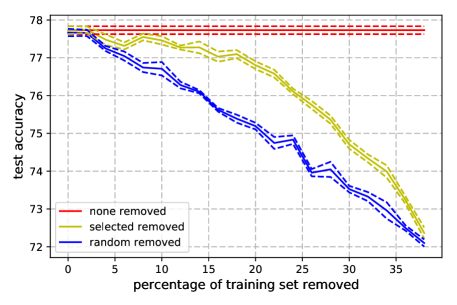
Our experimental findings suggest that: a) there exist a large number of unforgettable examples, i.e., examples that are never forgotten once learnt, those examples are stable across seeds and strongly correlated from one neural architecture to another; b) examples with noisy labels are among the most forgotten examples, along with images with “uncommon” features, visually complicated to classify; c) training a neural network on a dataset where a very large fraction of the least forgotten examples have been removed still results in extremely competitive performance on the test set.
2 Related Work
Curriculum Learning and Sample Weighting
Curriculum learning is a paradigm that favors learning along a curriculum of examples of increasing difficulty (Bengio et al., 2009). This general idea has found success in a variety of areas since its introduction (Kumar et al., 2010; Lee & Grauman, 2011; Schaul et al., 2015). Kumar et al. (2010) implemented their curriculum by considering easy the examples with a small loss. Arpit et al. (2017) also pose that easy examples exist, and define them as those that are correctly classified after only epoch of training, though they do not examine whether these examples are later forgotten. In our experiments, we empirically validate that unforgettable examples can be safely removed without compromising generalization. Zhao & Zhang (2015); Katharopoulos & Fleuret (2018) relate sample importance to the norm of its loss gradient with respect to the parameters of the network. Fan et al. (2017); Kim & Choi (2018); Jiang et al. (2018) learn a curriculum directly from data in order to minimize the task loss. Jiang et al. (2018) also study the robustness of their method in the context of noisy examples. This relates to a rich literature on outlier detection and removal of examples with noisy labels (John, 1995; Brodley & Friedl, 1999; Sukhbaatar et al., 2014; Jiang et al., 2018). We will provide evidence that noisy examples rank higher in terms of number of forgetting events. Koh & Liang (2017) borrow influence functions from robust statistics to evaluate the impact of the training examples on a model’s predictions.
Deep Generalization
The study of the generalization properties of deep neural networks when trained by stochastic gradient descent has been the focus of several recent publications (Zhang et al., 2016; Keskar et al., 2016; Chaudhari et al., 2016; Advani & Saxe, 2017). These studies suggest that the generalization error does not depend solely on the complexity of the hypothesis space. For instance, it has been demonstrated that over-parameterized models with many more parameters than training points can still achieve low test error (Huang et al., 2017; Wang et al., 2018) while being complex enough to fit a dataset with completely random labels (Zhang et al., 2016). A possible explanation for this phenomenon is a form of implicit regularization performed by stochastic gradient descent: deep neural networks trained with SGD have been recently shown to converge to the maximum margin solution in the linearly separable case (Soudry et al., 2017; Xu et al., 2018). In our work, we provide empirical evidence that generalization can be maintained when removing a substantial portion of the training examples and without restricting the complexity of the hypothesis class. This goes along the support vector interpretation provided by Soudry et al. (2017).
3 Defining and Computing Example Forgetting
Our general case study for example forgetting is a standard classification setting. Given a dataset of observation/label pairs, we wish to learn the conditional probability distribution using a deep neural network with parameters . The network is trained to minimize the empirical risk , where denotes the cross-entropy loss and . The minimization is performed using variations of stochastic gradient descent, starting from initial random parameters , and by sampling examples at random from the dataset .
Forgetting and learning events We denote by the predicted label for example obtained after steps of SGD. We also let be a binary variable indicating whether the example is correctly classified at time step . Example undergoes a forgetting event when decreases between two consecutive updates: . In other words, example is misclassified at step after having been correctly classified at step . Conversely, a learning event has occurred if . Statistics that will be of interest in the next sections include the distribution of forgetting events across examples and the first time a learning event occurs.
Classification margin We will also be interested in analyzing the classification margin. Our predictors have the form , where is a sigmoid (softmax) activation function in the case of binary (categorical) classification. The classification margin is defined as the difference between the logit of the correct class and the largest logit among the other classes, i.e. , where is the index corresponding to the correct class.
Unforgettable examples We qualify examples as unforgettable if they are learnt at some point and experience no forgetting events during the whole course of training: example is unforgettable if the first time it is learnt verifies and for all , . Note that, according to this definition, examples that are never learnt during training do not qualify as unforgettable. We refer to examples that have been forgotten at least once as forgettable.
3.1 Procedural Description and Experimental Setting
Following the previous definitions, monitoring forgetting events entails computing the prediction for all examples in the dataset at each model update, which would be prohibitively expensive.
In practice, for each example, we subsample the full sequence of forgetting events by computing forgetting statistics only when the example is included in the current mini-batch; that is, we compute forgetting across presentations of the same example in subsequent mini-batches. This gives a lower bound on the number of forgetting events an example undergoes during training.
We train a classifier on a given dataset and record the forgetting events for each example when they are sampled in the current mini-batch. For the purposes of further analysis, we then sort the dataset’s examples based on the number of forgetting events they undergo. Ties are broken at random when sampling from the ordered data. Samples that are never learnt are considered forgotten an infinite number of times for sorting purposes. Note that this estimate of example forgetting is computationally expensive; see Sec. 6 for a discussion of a cheaper method.
We perform our experimental evaluation on three datasets of increasing complexity: MNIST (LeCun et al., 1999), permuted MNIST – a version of MNIST that has the same fixed permutation applied to the pixels of all examples, and CIFAR-10 (Krizhevsky, 2009). We use various model architectures and training schemes that yield test errors comparable with the current state-of-the-art on the respective datasets. In particular, the MNIST-based experiments use a network comprised of two convolutional layers followed by a fully connected one, trained using SGD with momentum and dropout. This network achieves 0.8% test error. For CIFAR-10, we use a ResNet with cutout (DeVries & Taylor, 2017) trained using SGD and momentum with a particular learning rate schedule. This network achieves a competitive 3.99% test error. For full experimentation details, see the Supplementary.
4 Characterizing Example Forgetting
Number of forgetting events
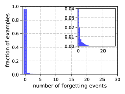
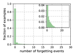
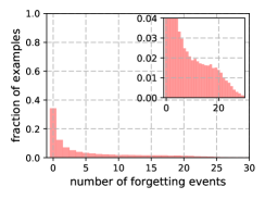
We estimate the number of forgetting events of all the training examples for the three different datasets (MNIST, permutedMNIST and CIFAR-10) across 5 random seeds. The histograms of forgetting events computed from one seed are shown in Figure 1. There are , and unforgettable examples common across seeds, they represent respectively , , and of the corresponding training sets. Note that datasets with less complexity and diversity of examples, such as MNIST, seem to contain significantly more unforgettable examples. permutedMNIST exhibits a complexity balanced between MNIST (easiest) and CIFAR-10 (hardest). This finding seems to suggest a correlation between forgetting statistics and the intrinsic dimension of the learning problem, as recently formalized by Li et al. (2018).
Stability across seeds To test the stability of our metric with respect to the variance generated by stochastic gradient descent, we compute the number of forgetting events per example for different random seeds and measure their correlation. From one seed to another, the average Pearson correlation is . When randomly splitting the different seeds into two sets of , the cumulated number of forgetting events within those two sets shows a high correlation of . We also ran the original experiment on 100 seeds to devise 95% confidence bounds on the average (over 5 seeds) number of forgetting events per example (see Appendix 13). The confidence interval of the least forgotten examples is tight, confirming that examples with a small number of forgetting events can be ranked confidently.
Forgetting by chance In order to quantify the possibility of forgetting occurring by chance, we additionally analyze the distribution of forgetting events obtained under the regime of random update steps instead of the true SGD steps. In order to maintain the statistics of the random updates similar to those encountered during SGD, random updates are obtained by shuffling the gradients produced by standard SGD on a main network (more details are provided in Appendix 12). We report the histogram of chance forgetting events in Supplementary Figure 13: examples are being forgotten “by chance” a small number of time, at most twice and most of the time less than once. The observed stability across seeds, low number of chance forgetting events and the tight confidence bounds suggest that it is unlikely for the ordering produced by the metric to be the by-product of another unrelated random cause.
First learning events
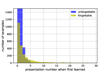
We investigate whether unforgettable and forgettable examples need to be presented different numbers of times in order to be learnt for the first time (i.e. for the first learning event to occur, as defined in Section 3). The distributions of the presentation numbers at which first learning events occur across all datasets can be seen in Supplemental Figure 8. We observe that, while both unforgettable and forgettable sets contain many examples that are learnt during the first - presentations, the forgettable examples contain a larger number of examples that are first learnt later in training. The Spearman rank correlation between the first learning event presentations and the number of forgetting events across all training examples is , indicating a moderate relationship.
Misclassification margin
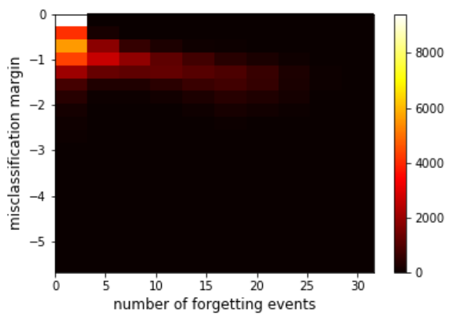
The definition of forgetting events is binary and as such fairly crude compared to more sophisticated estimators of example relevance (Zhao & Zhang, 2015; Chang et al., 2017). In order to qualify its validity, we compute the misclassification margin of forgetting events. The misclassification margin of an example is defined as the mean classification margin (defined in Section 3) over all its forgetting events, a negative quantity by definition. The Spearman rank correlation between an example’s number of forgetting events and its mean misclassification margin is -0.74 (computed over 5 seeds, see corresponding 2D-histogram in Supplemental Figure 9). These results suggest that examples which are frequently forgotten have a large misclassification margin.

Visual inspection
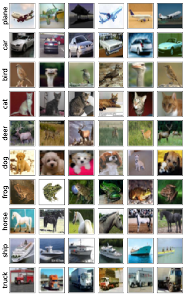
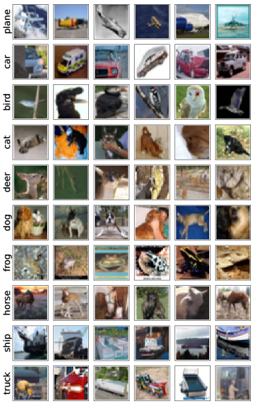
We visualize some of the unforgettable examples in Figure 2 along with some examples that have been most forgotten in the CIFAR-10 dataset. Unforgettable samples are easily recognizable and contain the most obvious class attributes or centered objects, e.g., a plane on a clear sky. On the other hand, the most forgotten examples exhibit more ambiguous characteristics (as in the center image, a truck on a brown background) that may not align with the learning signal common to other examples from the same class.
Detection of noisy examples
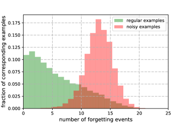
We further investigate the observation that the most forgettable examples seem to exhibit atypical characteristics. We would expect that if highly forgettable examples have atypical class characteristics, then noisily-labeled examples will undergo more forgetting events. We randomly change the labels of of CIFAR-10 and record the number of forgetting events of both the noisy and regular examples through training. The distributions of forgetting events across noisy and regular examples are shown in Figure 3. We observe that the most forgotten examples are those with noisy labels and that no noisy examples are unforgettable. We also compare the forgetting events of the noisy examples to that of the same set of examples with original labels and observe a much higher degree of forgetting in the noisy case. The results of these synthetic experiments support the hypothesis that highly forgettable examples exhibit atypical class characteristics.
4.1 Continual Learning Setup
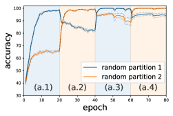
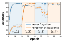
We observed that in harder tasks such as CIFAR-10, a significant portion of examples are forgotten at least once during learning. This leads us to believe that catastrophic forgetting may be observed, to some extent, even when considering examples coming from the same task distribution. To test this hypothesis, we perform an experiment inspired by the standard continual learning setup (McCloskey & Cohen, 1989; Kirkpatrick et al., 2017). We create two tasks by randomly sampling 10k examples from the CIFAR-10 training set and dividing them in two equally-sized partitions (5k examples each). We treat each partition as a separate ”task” even though they should follow the same distribution. We then train a classifier for 20 epochs on each partition in an alternating fashion, while tracking performance on both partitions. The results are reported in Figure 4 (a). The background color represents which of the two partitions is currently used for training. We observe some forgetting of the second task when we only train on the first task (panel (a.2)). This is somewhat surprising as the two tasks contain examples from the same underlying distribution.
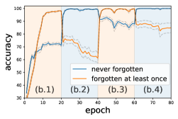
We contrast the results from training on random partitions of examples with ones obtained by partitioning the examples based on forgetting statistics (Figure 4 (b)). That is, we first compute the forgetting events for all examples based on Algorithm 1 and we create our tasks by sampling 5k examples that have zero forgetting events (named f0) and 5k examples that have non-zero forgetting events (named fN). We observe that examples that have been forgotten at least once suffer a more drastic form of forgetting than those included in a random split (compare (a.2) with (b.2)). In panel (b.3) and (c.2) we can observe that examples from task f0 suffer very mild forgetting when training on task fN. This suggests that examples that have been forgotten at least once may be able to “support” those that have never been forgotten. We observe the same pattern when we investigate the opposite alternating sequence of tasks in Figure 4 (b, right).
5 Removing Unforgettable Examples
As shown in the previous section, learning on examples that have been forgotten at least once minimally impacts performance on those that are unforgettable. This appears to indicate that unforgettable examples are less informative than others, and, more generally, that the more an example is forgotten during training, the more useful it may be to the classification task. This seems to align with the observations in Chang et al. (2017), where the authors re-weight training examples by accounting for the variance of their predictive distribution. Here, we test whether it is possible to completely remove a given subset of examples during training.
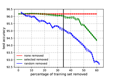
In Fig. 5 (Left), we show the evolution of the generalization performance in CIFAR-10 when we artificially remove examples from the training dataset. We choose the examples to remove by increasing number of forgetting events. Each point in the figure corresponds to retraining the model from scratch on an increasingly smaller subset of the training data (with the same hyper-parameters as the base model). We observe that when removing a random subset of the dataset, performance rapidly decreases. Comparatively, by removing examples ordered by number of forgetting events, of the dataset can be removed while maintaining comparable generalization performance as the base model trained on the full dataset, and up to can be removed with marginal degradation (less than ). The results on the other datasets are similar: a large fraction of training examples can be ignored without hurting the final generalization performance of the classifiers (Figure 6).
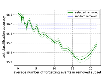
In Figure 5 (Right), we show the evolution of the generalization error when we remove from the dataset examples with increasing forgetting statistics. Each point in the figure corresponds to the generalization error of a model trained on the full dataset minus examples as a function of the average number of forgetting events in those examples. As can be seen, removing the same number of examples with increasingly more forgetting events results in worse generalization for most of the curve. It is interesting to notice the rightmost part of the curve moving up, suggesting that some of the most forgotten examples actually hurt performance. Those could correspond to outliers or mislabeled examples (see Sec. 4). Finding a way to separate those points from very informative ones is an ancient but still active area of research (John, 1995; Jiang et al., 2018).
Support vectors Various explanations of the implicit generalization of deep neural networks (Zhang et al., 2016) have been offered: flat minima generalize better and stochastic gradient descent converges towards them (Hochreiter & Schmidhuber, 1997; Kleinberg et al., 2018), gradient descent protects against overfitting (Advani & Saxe, 2017; Tachet et al., 2018), deep networks’ structure biases learning towards simple functions (Neyshabur et al., 2014; Perez et al., 2018). But it remains a poorly understood phenomenon. An interesting direction of research is to study the convergence properties of gradient descent in terms of maximum margin classifiers. It has been shown recently (Soudry et al., 2017) that on separable data, a linear network will learn such a maximum margin classifier. This supports the idea that stochastic gradient descent implicitly converges to solutions that maximally separate the dataset, and additionally, that some data points are more relevant than others to the decision boundary learnt by the classifier. Those points play a part equivalent to support vectors in the support vector machine paradigm. Our results confirm that a significant portion of training data points have little to no influence on the generalization performance when the decision function is learnt with SGD. Forgettable training points may be considered as analogs to support vectors, important for the generalization performance of the model. The number of forgetting events of an example is a relevant metric to detect such support vectors. It also correlates well with the misclassification margin (see Sec.4) which is a proxy for the distance to the decision boundary.
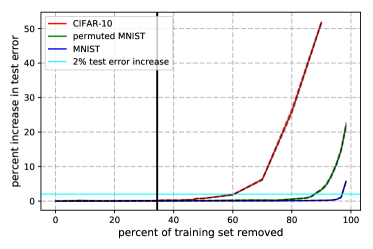
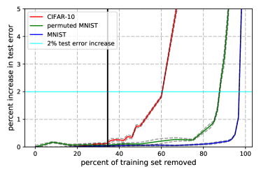
Intrinsic dataset dimension As mentioned above, the datasets we study have various fractions of unforgettable events ( for MNIST, for permutedMNIST and for CIFAR-10). We also see in Figure 6 that performance on those datasets starts to degrade at different fractions of removed examples: the number of support vectors varies from one dataset to the other, based on the complexity of the underlying data distribution. If we assume that we are in fact detecting analogs of support vectors, we can put these results in perspective with the intrinsic dataset dimension defined by Li et al. (2018) as the codimension in the parameter space of the solution set: for a given architecture, the higher the intrinsic dataset dimension, the larger the number of support vectors, and the fewer the number of unforgettable examples.
6 Transferable Forgetting Events
Forgetting events rely on training a given architecture, with a given optimizer, for a given number of epochs. We investigate to what extent the forgetting statistics of examples depend on those factors.
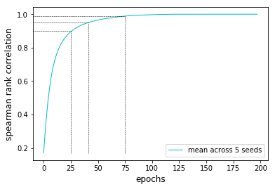
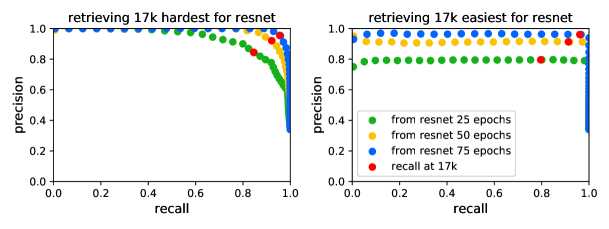
Throughout training We compute the Spearman rank correlation between the ordering obtained at the end of training ( epochs) and the ordering after various number of epochs. As seen in Fig. 7 (Left), the ordering is very stable after epochs, and we found a reasonable number of epochs to get a good correlation to be 25 (see the Supplementary Materials for precision-recall plots).
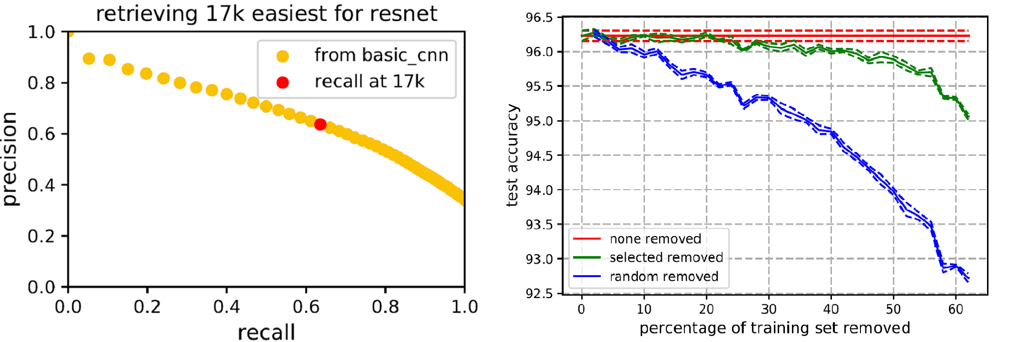
Between architectures A limitation of our method is that it requires computing the ordering from a previous run. An interesting question is whether that ordering could be obtained from a simpler architecture than residual networks. We train a network with two convolutional layers followed by two fully connected ones (see the Supplementary for the full architecture) and compare the resulting ordering with the one obtained with ResNet18. Figure 7 (Middle) shows a precision-recall plot of the unforgettable examples computed with the residual network. We see a reasonably strong agreement between the unforgettable examples of the convolutional neural network and the ones of the ResNet18. Finally, we train a WideResNet (Zagoruyko & Komodakis, 2016) on truncated data sets using the example ordering from ResNet18. Using the same computing power (one Titan X GPU), Resnet18 requires hours to train whereas WideResNet requires – estimating the forgetting statistics of WideResNet via ResNet18 can save up to hours of training time if the estimate is accurate. We plot WideResNet’s generalization performance using the ordering obtained by ResNet18 in Figure 7 (Right): the network still performs near optimally with of the dataset removed. This opens up promising avenues of computing forgetting statistics with smaller architectures.
7 Conclusion and Future Work
In this paper, inspired by the phenomenon of catastrophic forgetting, we investigate the learning dynamics of neural networks when training on single classification tasks. We show that catastrophic forgetting can occur in the context of what is usually considered to be a single task. Inspired by this result, we find that some examples within a task are more prone to being forgotten, while others are consistently unforgettable. We also find that forgetting statistics seem to be fairly stable with respect to the various characteristics of training, suggesting that they actually uncover intrinsic properties of the data rather than idiosyncrasies of the training schemes. Furthermore, the unforgettable examples seem to play little part in the final performance of the classifier as they can be removed from the training set without hurting generalization. This supports recent research interpreting deep neural networks as max margin classifiers in the linear case. Future work involves understanding forgetting events better from a theoretical perspective, exploring potential applications to other areas of supervised learning, such as speech or text and to reinforcement learning where forgetting is prevalent due to the continual shift of the underlying distribution.
8 Acknowledgments
We acknowledge the anonymous reviewers for their insightful suggestions.
References
- Advani & Saxe (2017) Madhu S. Advani and Andrew M. Saxe. High-dimensional dynamics of generalization error in neural networks. CoRR, abs/1710.03667, 2017.
- Arpit et al. (2017) Devansh Arpit, Stanislaw Jastrzebski, Nicolas Ballas, David Krueger, Emmanuel Bengio, Maxinder S Kanwal, Tegan Maharaj, Asja Fischer, Aaron Courville, Yoshua Bengio, et al. A closer look at memorization in deep networks. In Proceedings of the 34th International Conference on Machine Learning-Volume 70, pp. 233–242. JMLR.org, 2017.
- Bengio & LeCun (2007) Yoshua Bengio and Yann LeCun. Scaling learning algorithms towards AI. In Large Scale Kernel Machines. MIT Press, 2007.
- Bengio et al. (2009) Yoshua Bengio, Jérôme Louradour, Ronan Collobert, and Jason Weston. Curriculum learning. In Proceedings of the 26th annual international conference on machine learning, pp. 41–48. ACM, 2009.
- Brodley & Friedl (1999) Carla E Brodley and Mark A Friedl. Identifying mislabeled training data. Journal of artificial intelligence research, 11:131–167, 1999.
- Chang et al. (2017) Haw-Shiuan Chang, Erik Learned-Miller, and Andrew McCallum. Active Bias: Training More Accurate Neural Networks by Emphasizing High Variance Samples. In Advances in Neural Information Processing Systems, pp. 1002–1012, 2017.
- Chaudhari et al. (2016) Pratik Chaudhari, Anna Choromanska, Stefano Soatto, Yann LeCun, Carlo Baldassi, Christian Borgs, Jennifer Chayes, Levent Sagun, and Riccardo Zecchina. Entropy-SGD: Biasing Gradient Descent Into Wide Valleys. ICLR ’17, 2016.
- DeVries & Taylor (2017) Terrance DeVries and Graham W Taylor. Improved regularization of convolutional neural networks with cutout. arXiv preprint arXiv:1708.04552, 2017.
- Fan et al. (2017) Yang Fan, Fei Tian, Tao Qin, and Jiang Bian. Learning What Data to Learn. arXiv preprint arXiv:1702.08635, 2017.
- Finn et al. (2017) Chelsea Finn, Pieter Abbeel, and Sergey Levine. Model-agnostic meta-learning for fast adaptation of deep networks. In Proc. of ICML, 2017.
- Hochreiter & Schmidhuber (1997) S. Hochreiter and J. Schmidhuber. Flat minima. Neural Computation, 9(1):1–42, 1997.
- Huang et al. (2017) Gao Huang, Zhuang Liu, Laurens van der Maaten, and Kilian Q Weinberger. Densely Connected Convolutional Networks. In Proceedings of the IEEE Conference on Computer Vision and Pattern Recognition, pp. 4700–4708, 2017.
- Jiang et al. (2018) Lu Jiang, Zhengyuan Zhou, Thomas Leung, Li-Jia Li, and Li Fei-Fei. MentorNet: Learning data-driven curriculum for very deep neural networks on corrupted labels. In Proceedings of the 35th International Conference on Machine Learning. PMLR, 2018.
- John (1995) George H John. Robust decision trees: removing outliers from databases. In Proceedings of the First International Conference on Knowledge Discovery and Data Mining, pp. 174–179. AAAI Press, 1995.
- Katharopoulos & Fleuret (2018) Angelos Katharopoulos and François Fleuret. Not all samples are created equal: Deep learning with importance sampling. In Jennifer G. Dy and Andreas Krause (eds.), ICML, volume 80 of JMLR Workshop and Conference Proceedings, pp. 2530–2539. JMLR.org, 2018. URL http://dblp.uni-trier.de/db/conf/icml/icml2018.html#KatharopoulosF18.
- Keskar et al. (2016) Nitish Shirish Keskar, Dheevatsa Mudigere, Jorge Nocedal, Mikhail Smelyanskiy, and Ping Tak Peter Tang. On large-batch training for deep learning: Generalization gap and sharp minima. arXiv preprint arXiv:1609.04836, 2016.
- Kim & Choi (2018) Tae-Hoon Kim and Jonghyun Choi. Screenernet: Learning curriculum for neural networks. CoRR, abs/1801.00904, 2018. URL http://dblp.uni-trier.de/db/journals/corr/corr1801.html#abs-1801-00904.
- Kingma & Ba (2014) Diederik Kingma and Jimmy Ba. Adam: A method for stochastic optimization, 2014. URL http://arxiv.org/abs/1412.6980. cite arxiv:1412.6980Comment: Published as a conference paper at the 3rd International Conference for Learning Representations, San Diego, 2015.
- Kirkpatrick et al. (2017) James Kirkpatrick, Razvan Pascanu, Neil Rabinowitz, Joel Veness, Guillaume Desjardins, Andrei A Rusu, Kieran Milan, John Quan, Tiago Ramalho, Agnieszka Grabska-Barwinska, and Others. Overcoming catastrophic forgetting in neural networks. Proceedings of the national academy of sciences, pp. 201611835, 2017.
- Kleinberg et al. (2018) Robert Kleinberg, Yuanzhi Li, and Yang Yuan. An alternative view: When does sgd escape local minima? CoRR, abs/1802.06175, 2018. URL http://dblp.uni-trier.de/db/journals/corr/corr1802.html#abs-1802-06175.
- Koh & Liang (2017) Pang Wei Koh and Percy Liang. Understanding black-box predictions via influence functions. In Doina Precup and Yee Whye Teh (eds.), ICML, volume 70 of JMLR Workshop and Conference Proceedings, pp. 1885–1894. JMLR.org, 2017. URL http://dblp.uni-trier.de/db/conf/icml/icml2017.html#KohL17.
- Krizhevsky (2009) Alex Krizhevsky. Learning multiple layers of features from tiny images. Technical report, 2009. URL https://www.cs.toronto.edu/~kriz/learning-features-2009-TR.pdf.
- Kumar et al. (2010) M Pawan Kumar, Benjamin Packer, and Daphne Koller. Self-Paced Learning for Latent Variable Models. In Proc. of NIPS, pp. 1–9, 2010.
- LeCun et al. (1999) Y. LeCun, C. Cortes C., and C. Burges. The mnist database of handwritten digits. http://yann.lecun.com/exdb/mnist/, 1999.
- Lee & Grauman (2011) Yong Jae Lee and Kristen Grauman. Learning the easy things first: Self-paced visual category discovery. In Computer Vision and Pattern Recognition (CVPR), 2011 IEEE Conference on, pp. 1721–1728. IEEE, 2011.
- Li et al. (2018) Chunyuan Li, Heerad Farkhoor, Rosanne Liu, and Jason Yosinski. Measuring the intrinsic dimension of objective landscapes. CoRR, abs/1804.08838, 2018. URL http://dblp.uni-trier.de/db/journals/corr/corr1804.html#abs-1804-08838.
- McCloskey & Cohen (1989) Michael McCloskey and Neal J Cohen. Catastrophic interference in connectionist networks: The sequential learning problem. In Psychology of learning and motivation, volume 24, pp. 109–165. Elsevier, 1989.
- Neyshabur et al. (2014) Behnam Neyshabur, Ryota Tomioka, and Nathan Srebro. In search of the real inductive bias: On the role of implicit regularization in deep learning. CoRR, abs/1412.6614, 2014. URL http://dblp.uni-trier.de/db/journals/corr/corr1412.html#NeyshaburTS14.
- Perez et al. (2018) Guillermo Valle Perez, Chico Q. Camargo, and Ard A. Louis. Deep learning generalizes because the parameter-function map is biased towards simple functions. CoRR, abs/1805.08522, 2018. URL http://dblp.uni-trier.de/db/journals/corr/corr1805.html#abs-1805-08522.
- Ravi & Larochelle (2017) Sachin Ravi and Hugo Larochelle. Optimization as a model for few-shot learning. In Proc. of ICLR, 2017.
- Ritter et al. (2018) Hippolyt Ritter, Aleksandar Botev, and David Barber. Online Structured Laplace Approximations For Overcoming Catastrophic Forgetting. arxiv preprint arxiv: 1805.07810, 2018. URL http://arxiv.org/abs/1805.07810.
- Schaul et al. (2015) Tom Schaul, John Quan, Ioannis Antonoglou, and David Silver. Prioritized experience replay. arXiv preprint arXiv:1511.05952, 2015.
- Soudry et al. (2017) Daniel Soudry, Elad Hoffer, Mor Shpigel Nacson, Suriya Gunasekar, and Nathan Srebro. The Implicit Bias of Gradient Descent on Separable Data. arXiv preprint arxiv:1710.10345, 2017. URL http://arxiv.org/abs/1710.10345.
- Sukhbaatar et al. (2014) Sainbayar Sukhbaatar, Joan Bruna, Manohar Paluri, Lubomir Bourdev, and Rob Fergus. Training convolutional networks with noisy labels. arXiv preprint arXiv:1406.2080, 2014.
- Tachet et al. (2018) R. Tachet, M. Pezeshki, S. Shabanian, A. Courville, and Y. Bengio. On the learning dynamics of deep neural networks. arxiv preprint arxiv:1809.06848, 2018. doi: arXiv:1809.06848v1. URL https://arxiv.org/abs/1809.06848.
- Wang et al. (2018) Huan Wang, Nitish Shirish Keskar, Caiming Xiong, and Richard Socher. Identifying Generalization Properties in Neural Networks. arXiv preprint arXiv:1809.07402, pp. 1–23, 2018. doi: arXiv:1809.07402v1. URL http://arxiv.org/abs/1809.07402.
- Xu et al. (2018) Tengyu Xu, Yi Zhou, Kaiyi Ji, and Yingbin Liang. Convergence of sgd in learning relu models with separable data. CoRR, abs/1806.04339, 2018. URL http://dblp.uni-trier.de/db/journals/corr/corr1806.html#abs-1806-04339.
- Zagoruyko & Komodakis (2016) Sergey Zagoruyko and Nikos Komodakis. Wide residual networks, 2016. URL http://arxiv.org/abs/1605.07146. cite arxiv:1605.07146.
- Zhang et al. (2016) Chiyuan Zhang, Samy Bengio, Moritz Hardt, Benjamin Recht, and Oriol Vinyals. Understanding deep learning requires rethinking generalization. arXiv preprint arXiv:1611.03530, 2016.
- Zhao & Zhang (2015) Peilin Zhao and Tong Zhang. Stochastic Optimization with Importance Sampling for Regularized Loss Minimization. In Proc. of ICML, 2015.
9 Experimentation Details
Detailed distributions
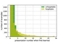
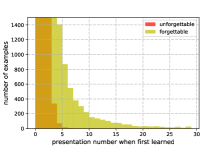
Misclassification margin
permutedMNIST The permutedMNIST data set is obtained by applying a fixed random permutation of the pixels to all the images of the standard MNIST data set. This typically makes the data set harder to learn for convolutional neural networks as local patterns, e.g. the horizontal bar of the , get shuffled. This statement is supported by the two following facts:
-
•
The number of unforgettable examples for permutedMNIST is 45181 versus 55012 for MNIST.
-
•
The intrinsic data set dimension (Li et al., 2018) of permutedMNIST is 1400 compared to 290 for the untouched data set.
Network Architectures We use a variety of different architectures in the main text. Below are their specifications.
The architecture for the MNIST and permutedMNIST experiments is the following:
-
1.
a first convolutional layer with 5 by 5 filters and 10 feature maps,
-
2.
a second convolutional layer with 5 by 5 filters and 20 feature maps,
-
3.
a fully connected layer with 50 hidden units
-
4.
the output layer, with 10 logits, one for each class.
We apply ReLU nonlinearities to the feature maps and to the hidden layer. The last layer is passed through a softmax to output probabilities for each class of the data set.
The ResNet18 architecture used for CIFAR-10 is described thoroughly in DeVries & Taylor (2017), its implementation can be found at https://github.com/uoguelph-mlrg/Cutout.
The second one is a WideResNet (Zagoruyko & Komodakis, 2016), with a depth of 28 and a widen factor of 10. We used the implementation found at https://github.com/meliketoy/wide-resnet.pytorch.
The convolutional architecture used in Section 6 is the following:
-
1.
a first convolutional layer with 5 by 5 filters and 6 feature maps,
-
2.
a 2 by 2 max pooling layer
-
3.
a second convolutional layer with 5 by 5 filters and 16 feature maps,
-
4.
a first fully connected layer with 120 hidden units
-
5.
a second fully connected layer with 84 hidden units
-
6.
the output layer, with 10 logits, one for each class.
Optimization
The MNIST networks are trained to minimize the cross-entropy loss using stochastic gradient descent with a learning rate of and a momentum of .
The ResNet18 is trained using cutout, data augmentation and stochastic gradient descent with a Nesterov momentum and a learning rate starting at 0.1 and divided by 5 at epochs , and .
The WideResNet is trained using Adam (Kingma & Ba, 2014) and a learning rate of .
10 Stability of the forgetting events
In Fig 10, we plot precision-recall diagrams for the unforgettable and most forgotten examples of CIFAR-10 obtained on ResNet18 after 200 epochs and various prior time steps. We see in particular that at 75 epochs, the examples on both side of the spectrum can be retrieved with very high precision and recall.
11 Noising the data sets
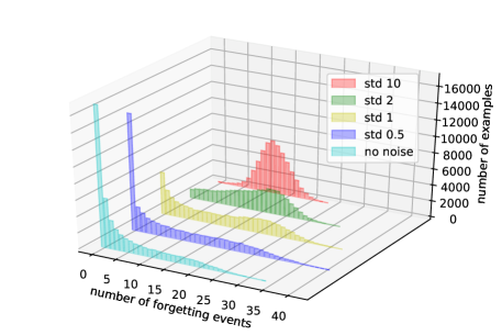
In Section 4, we analyzed the effect of adding label noise on the distribution of forgetting events. Here, we examine the effect of adding pixel noise, i.e. noising the input distribution. We choose to corrupt the inputs with additive Gaussian noise with zero mean and we choose for its standard deviation to be a multiple of channel-wise data standard deviation (i.e., ). Note that we add the noise after applying a channel-wise standard normalization step of the training images, therefore (each channel has zero mean, unit variance, this is a standard pre-processing step and has been applied throughout all the experiments in this paper).
The forgetting distributions obtained by noising all the dataset examples with increasing noise standard deviation are presented in Figure 11. We observe that adding increasing amount of noise decreases the amount of unforgettable examples and increases the amount of examples in the second mode of the forgetting distribution.
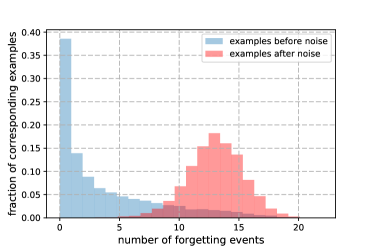
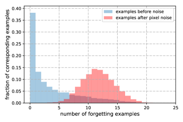
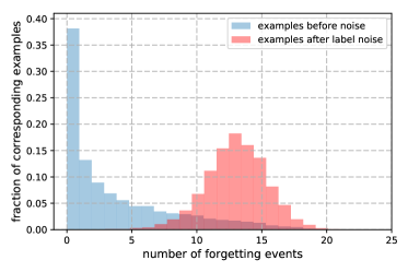
We follow the noisy-labels experiments of Section 4 and we apply the aforementioned pixel noise to of the training data (). We present the results of comparing the forgetting distribution of the of examples before and after noise was added to the pixels in Figure 12 (Left). For ease of comparison, we report the same results in the case of label noise in Figure 12 (Right). We observe that the forgetting distribution under pixel noise resembles the one under label noise.
12 ”Chance” forgetting events on CIFAR-10
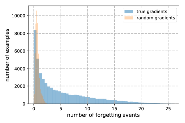
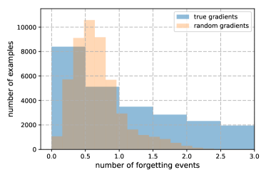
Forgetting events may happen by “chance”, i.e. some learning/forgetting events may occur even with random gradients. In order to estimate how large the effect of “chance” is, we compute the forgetting events of a classifier obtained by randomizing the update steps. To keep the statistics of the gradients similar to those encountered during SGD, we proceed as follows:
-
1.
Before the beginning of training, clone the “base” classifier into a new “clone” classifier with the same random weights.
-
2.
At each training step, shuffle the gradients computed on the base classifier and apply those to the clone (the base classifier is still optimized the same way): this ensures that the statistics of the random updates match the statistics of the true gradients during learning.
-
3.
Compute the forgetting events of the clone classifier on the training set exactly as is done with the base classifier.
The results can be found in Fig 13, showing the histogram of forgetting events produced by the “clone” network, averaged over 5 seeds. This gives an idea of the chance forgetting rate across examples. In this setting, examples are being forgotten “by chance” at most twice.
13 Confidence on forgetting events for CIFAR-10
In order to establish confidence intervals on the number of forgetting events, we computed them on 100 seeds and formed 20 averages over 5 seeds. In Fig 14, we show the average (in green), the bottom 2.5 percentile (in blue) and top 2.5 percentile (in orange) of those 20 curves.
![[Uncaptioned image]](/html/1812.05159/assets/forg_event_confidence_5_seeds.png)
14 Visualization of forgettable and unforgettable images
See Fig 15 for additional pictures of the most unforgettable and forgettable examples of every CIFAR-10 class, when examples are sorted by number of forgetting events (ties are broken randomly).
15 Forgetting in CIFAR-100
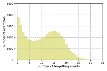
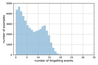
The distribution of forgetting events in CIFAR-100 is shown in Figure 16. There are unforgettable examples ( of the training set). CIFAR-100 is the hardest to classify out all of the presented datasets and exhibits the highest percentage of forgetting events. This finding further supports the idea that there may be a correlation between the forgetting statistics and the intrinsic dimension of the learning problem. Additionally, each CIFAR-100 class contains 10 times fewer examples than in CIFAR-10 or the MNIST datasets, making each image all the more useful for the learning problem.
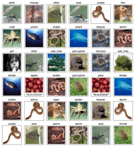
We also observe that the distribution of forgetting in CIFAR-100 is much closer to that of forgetting in the noisy CIFAR-10 than it is to forgetting in the original datasets presented in Figure 1. Visualizing the most forgotten examples in CIFAR-100 revealed that CIFAR-100 contains several images that appear multiple times in the training set under different labels. In Figure 17, we present the most forgotten examples in CIFAR-100. Note that they are all images that appear under multiple labels (not shown: the ”girl” image also appears under the label ”baby”, the ”mouse” image also appears under ”shrew”, one of the images of ‘oak_tree’ appears under ‘willow_tree’ and the other under ’maple_tree’).
We perform the same removal experiments we presented in Figure 5 for CIFAR-100. The results are shown in Figure 18. Just like with CIFAR-10, we are able to remove all unforgettable examples ( of the training set) while maintaining test performance.
