The Disk Substructures at High Angular Resolution Project (DSHARP)
VI: Dust trapping in thin-ringed protoplanetary disks

Abstract

A large fraction of the protoplanetary disks observed with ALMA display multiple well-defined and nearly perfectly circular rings in the continuum, in many cases with substantial peak-to-valley contrast. The DSHARP campaign shows that several of these rings are very narrow in radial extent. In this paper we test the hypothesis that these dust rings are caused by dust trapping in radial pressure bumps, and if confirmed, put constraints on the physics of the dust trapping mechanism. We model this process analytically in 1D, assuming axisymmetry. By comparing this model to the data, we find that all rings are consistent with dust trapping. Based on a plausible model of the dust temperature we find that several rings are narrower than the pressure scale height, providing strong evidence for dust trapping. The rings have peak absorption optical depth in the range between 0.2 and 0.5. The dust masses stored in each of these rings is of the order of tens of Earth masses, though much ambiguity remains due to the uncertainty of the dust opacities. The dust rings are dense enough to potentially trigger the streaming instability, but our analysis cannot give proof of this mechanism actually operating. Our results show, however, that the combination of very low $\alpha_{\mathrm{turb}}\ll 5\times 10^{-4}$ and very large grains $a_{\mathrm{grain}}\gg 0.1\,\mathrm{cm}$ can be excluded by the data for all the rings studied in this paper.

1 Introduction

The concept of dust trapping in local pressure maxima has become a central theme in studies of planet formation and protoplanetary disk evolution, because it might provide an elegant solution to several problems in these fields of study. Theories of planet formation are plagued by the “radial drift barrier”: the problem that, as dust aggregates grow by coagulation, they tend to radially drift toward the star before they reach planetesimal size (e.g. Birnstiel et al., 2010). A natural solution to this problem could be the trapping of dust particles in local pressure maxima (Whipple, 1972; Kretke & Lin, 2007; Barge & Sommeria, 1995; Klahr & Henning, 1997). Not only does this process prevent excessive radial drift of dust particles, it also tends to concentrate the dust into small volumes and high dust-to-gas ratios, which is beneficial to planet formation. From an observational perspective, the radial drift problem manifests itself by the presence of large grains in the outer regions of protoplanetary disks (Testi et al., 2003; Andrews et al., 2009; Ricci et al., 2010), which appears to be in conflict with theoretical predictions (Brauer et al., 2007). One possible solution to this observational conundrum could be that the disks are much more massive in the gas than previously suspected, leading to a higher gas friction for millimeter grains and thus longer drift time scales (Powell et al., 2017).

Another explanation is to invoke dust traps. The most striking observational evidence for dust trapping seems to come from large transitional disks, which feature giant dust rings, sometimes lopsided, in which large quantities of dust appears to be concentrated (Casassus et al., 2013; van der Marel et al., 2013). These observations appear to be well explained by the dust trapping scenario (Pinilla et al., 2012a). But these transitional disks seem to be rather violent environments, possibly with strong warps (Marino et al., 2015; Benisty et al., 2017) and companion-induced spirals (Dong et al., 2016).

For more “normal” protoplanetary disk the dust traps would have to be more subtle. Pinilla et al. (2012b) explored the possibility that the disk contains many axisymmetric local pressure maxima, and calculated how the dust drift and growth would behave under such conditions. It was found that, if the pressure bumps are strong enough, the dust trapping can keep a sufficient fraction of the dust mass at large distances from the star to explain the observed dust millimeter flux. It would leave, however, a detectable pattern of rings that should be discernable with ALMA observations. Since the multi-ringed disk observation of HL Tau (ALMA Partnership et al., 2015) a number of such multi-ringed disks have been detected (Andrews et al., 2016; Isella et al., 2016; Cieza et al., 2017; Fedele et al., 2017, 2018; Dipierro et al., 2018; van Terwisga et al., 2018; Clarke et al., 2018; Long et al., 2018). It is therefore very tempting to see also these multi-ringed disks as evidence for dust trapping, and as an explanation for the retention of dust in the outer regions of protoplanetary disks.

The data from the ALMA Large Programme DSHARP (Andrews, 2018) offers an exciting new opportunity to put this concept to the test, and to put constraints on the physics of dust trapping in axisymmetric pressure maxima. This is an opportunity which we explore in this paper.

As is shown by Huang (2018a), most of the disks in the DSHARP sample display multi-ringed substructure. We investigate whether these rings are caused by dust trapping, and if so, what we can learn about dust trapping from these data. We will focus on a subsample of rings, for which the contrast is particularly strong, so that amplitude and width can be clearly defined. We study the rings individually, assuming that the dust does not escape from the ring. This makes it possible to look for a steady-state dust trapping solution in which the radial drift forces (that push the dust to the pressure peak) are balanced by turbulent mixing (that tends to smear out the dust away from the pressure peak). In Appendix F we will construct a very simplified analytic dust trapping model, and confront this with the most well-isolated rings from our sample.

The structure of the paper is as follows. We first review, in Section 2, our subsample of rings, and how the radial profile of the intensity was obtained. Next we fit these rings to Gaussians (Section 3), because this will make the quantitative analysis of the subsequent sections easier. In Section 4.1 we will first analyze these Gaussian fits under the assumption that these rings are optically thin. It turns out, however, that the optical depths are on the border between thin and thick, requiring us to explore, in Section 4.2 how moderate optical depths affect our results, and correct for this. We are then ready to compare this to a model of dust trapping. In Section 5 we take the simplest possible model of dust trapping: that of a Gaussian pressure bump. This allows us to derive most results analytically. In Section 6 we go one step further by numerically exploring dust trapping by a very simple planetary gap model, and see to which extent the results are different and may fit better or worse to the data. We close with a discussion and conclusion section.

2 The high-contrast rings of AS 209, Elias 24, HD 163296, GW Lup and HD 143006

In this paper we focus on a subsample of sources of the DSHARP Programme that show high-contrast and radially thin rings that are separated by deep valleys, and that are sufficiently face-on to not have to worry much about 3-D line-of-sight issues. These are AS 209, Elias 24, HD 163296, GW Lup and HD 143006. Their stellar parameters are given in Table 1.

Table 1: The stellar parameters assumed for the stars studied in this paper, and the ALMA beam size and position angle of the DSHARP observations.

Source	$d$	$M_{*}$	$L_{*}$	$i$	Beam, PA
	[pc]	$[M_{\odot}]$	$[L_{\odot}]$	[deg]	[mas], [deg]
AS 209	121	0.83	1.41	35	38$\times$36, 68
Elias 24	136	0.78	6.0	29	37$\times$24, 82
HD 163296	101	2.04	17.0	47	48$\times$38, 82
GW Lup	155	0.46	0.33	39	45$\times$43, 1
HD 143006	165	1.78	3.80	19	46$\times$45, 51

Note. — Distance is in parsec and mass and luminosity are in units of the solar values. The beam is in milliarcsecond. Inclination and position angle are in degrees (PA east from north for the major axis). More details, as well as references and uncertainty estimates, can be found in Andrews (2018).

A gallery of these sources is shown in Fig. 1. For an overview of the ALMA Large Programme we refer to Andrews (2018), and for an in-depth discussion on the data of the individual sources we refer to Huang (2018a), Isella (2018), Guzmán (2018) and Perez (2018).

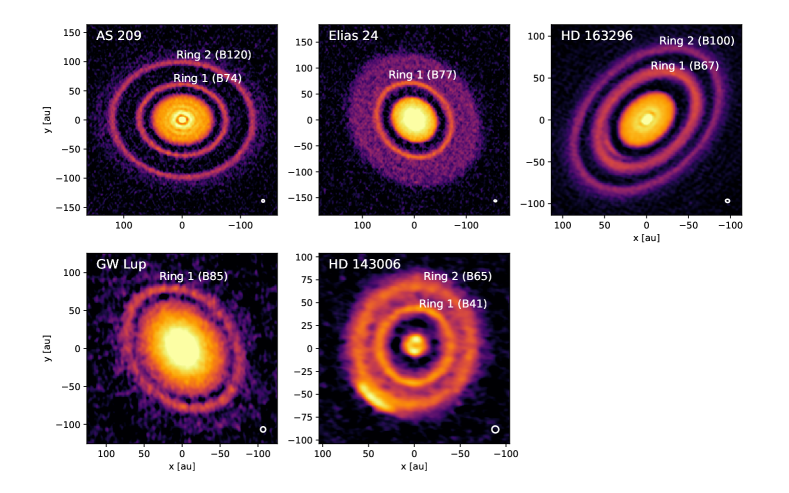
Figure 1: The continuum maps in band 6 of the five disks in our sample which have the most pronounced rings. The eight highest contrast rings, which are the topic of this paper, are marked in the images. The color scale is the same as from Huang (2018a). For a detailed description of these data, see Guzmán (2018) for AS 209, Isella (2018) for HD 163296, Perez (2018) for HD 143006, and Huang (2018a) for the rest.

The high-contrast rings of these sources provide “clean laboratories” for testing the theory of dust trapping in a ring-by-ring manner. Fig. 2 shows the radial profile (deprojected for inclination) of the thermal emission of the dust of the five disks. These brightness profiles are expressed as intensity $I_{\nu}$ in units of $\mathrm{Jy}/\mathrm{arcsec}^{2}$. The procedure used to extract these radial profiles from the continuum maps is described by Huang (2018a). In creating these profiles, the “arcs” seen in HD 163296 and HD 143006 were excised, so these radial profiles represent the axially symmetric structures only.

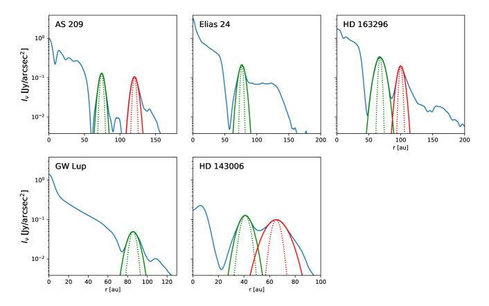
Figure 2: The intensity profiles in band 6 of the five disks in our sample which have the most pronounced rings. The vertical axis is logarithmic to better show the contrast. The eight highest contrast rings are fitted by a Gaussian profile, shown as the solid inverse parabolas. The dotted inverse parabolas are Gaussians with the width of the ALMA beam. For a detailed description of these data, see Huang (2018a). The unit of intensity is always $\mathrm{Jy/arcsec}^{2}$ at $\lambda=0.125\,\mathrm{cm}$. For Elias 24 the observations had a central wavelength of $\lambda=0.129\,\mathrm{cm}$, but we rescaled to $\lambda=0.125\,\mathrm{cm}$ assuming a spectral slope of $I_{\nu}\propto\nu^{2}$, meaning a 6.5% increase.

The DSHARP sample has many more sources with rings, and several of the sources we study in this paper display more than just the one or two rings we focus on (Huang, 2018a). Particularly striking in this regard is AS 209, which features three more ringlike structures in the inner disk. The contrast and radial separation of these rings is, however, much less than for the subset of rings we choose for this paper. While dust trapping can certainly also play a role in those rings, it is much harder to quantify this. For that reason we do not consider those rings further in this paper.

3 Fitting a Gaussian profile to the ring emission

As we will discuss later (Section 5), for a radially Gaussian pressure bump the solution to the radial dust mixing and drift problem is, to first approximation, also a Gaussian surface density profile. It has a width smaller than, or equal to, that of the gas pressure bump. Our analysis of the eight rings of this paper therefore naturally starts with the fitting of the observed radial intensity profiles with a Gaussian function. We choose here to do so in the image plane, because that allows us to select an individual ring, and study it independently of the emission elsewhere. But note that other papers in the DSHARP series have done, for individual sources, fits in the uv plane (Guzmán, 2018; Isella, 2018; Perez, 2018).

3.1 Procedure

The aim is to find, for each ring, a Gaussian intensity profile

$$I_{\nu}^{\mathrm{gauss}}(r)=A\,\exp\left(-\frac{(r-r_{0})^{2}}{2\sigma^{2}}\right)$$ (1)

that best describes the ring. To be more precise: We determine the values of $A$, $r_{0}$ and $\sigma$ for which Eq. (1) best fits the observed intensity profile $I_{\nu}^{\mathrm{obs}}(r)$ shown in Fig. 2 within a prescribed radial domain as given in Table 2. Details of the fitting procedure are described in Appendix B and C. The Gaussian fits appear as inverse parabolas in Fig. 2. In the close-up views of Fig. 3 they are overplotted in orange. The parameters of the best fits are listed in Tables 2 and 5.

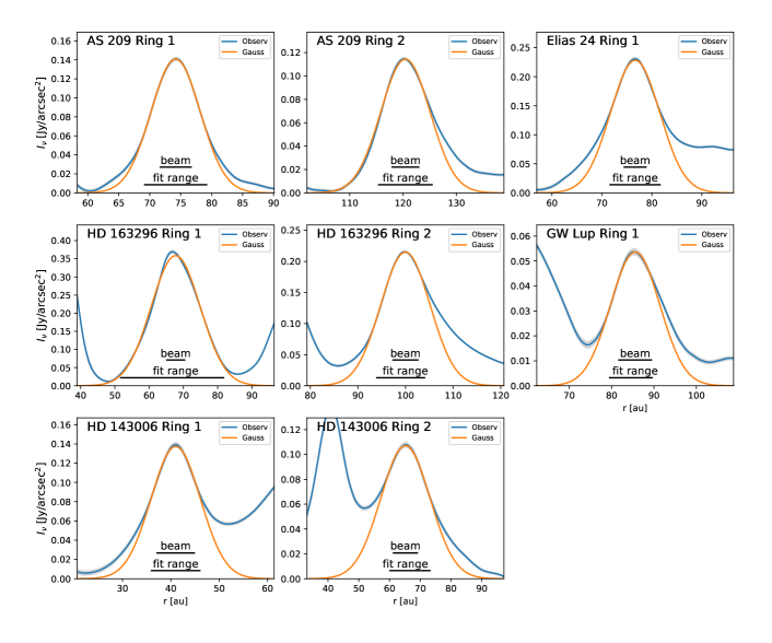
Figure 3: Gaussian fits to the eight rings of this paper. The blue curves are the observations, the orange curves are the best fit Gaussian profiles. The “fit range” bar shows the radial range within which the Gauss curve was fitted to the data. The fit range was chosen to fit the part of the curve that, by eye, most resembles a Gaussian. The “beam” bar shows the FWHM beam size of the observations. The grey band around the blue curve shows the estimated uncertainty of the data.

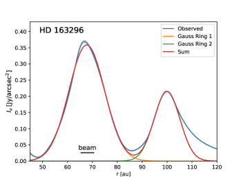
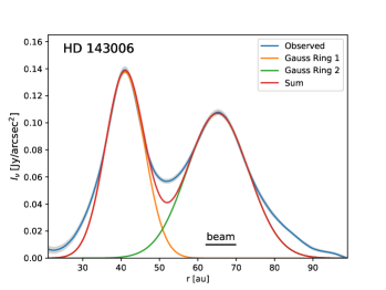
Figure 4: The sum of the two Gaussian fits for the two sources with two partly overlapping rings: HD 163296 and HD 143006.

Table 2: The model parameters for the Gaussian ring fits in Figs. 2 and 3

Source	Ring	Name	Beam	Domain	$A$	$A_{\mathrm{dec}}$	$r_{0}$	$\sigma$	$w_{d}$	$T_{\mathrm{d}}$	$B_{\nu}(T_{\mathrm{d}})$	$w_{d}/h_{p}$	$\sigma/\sigma_{b}$	$\tau_{\nu}^{\mathrm{peak}}$	$M_{\mathrm{d}}^{\mathrm{thin}}$	$M_{\mathrm{d}}^{\mathrm{true}}$
			$[\mathrm{mas}]$	$[\mathrm{au}]$	$[\mathrm{Jy/as}^{2}]$	$[\mathrm{Jy/as}^{2}]$	$[\mathrm{au}]$	$[\mathrm{au}]$	$[\mathrm{au}]$	$\mathrm{[K]}$	$[\mathrm{Jy/as}^{2}]$				$[M_{\oplus}]$	$[M_{\oplus}]$
(1)	(2)	(3)	(4)	(5)	(6)	(7)	(8)	(9)	(10)	(11)	(12)	(13)	(14)	(15)	(16)	(17)
AS 209	1	B74	40	69 – 79	0.14	0.17	74.2	3.98	3.38	15.8	0.45	0.6	1.9	0.46	27.0	31.5
AS 209	2	B120	40	115 – 125	0.11	0.13	120.4	4.62	4.11	12.4	0.32	0.4	2.2	0.52	58.7	69.8
Elias 24	1	B77	31	72 – 82	0.23	0.25	76.7	4.93	4.57	22.3	0.72	0.6	2.7	0.42	35.4	40.8
HD 163296	1	B67	51	52 – 82	0.36	0.38	67.7	7.18	6.84	30.8	1.06	1.6	3.2	0.44	48.3	56.0
HD 163296	2	B100	51	94 – 104	0.21	0.24	100.0	5.17	4.67	25.3	0.84	0.7	2.3	0.33	39.0	43.6
GW Lup	1	B85	49	79 – 89	0.05	0.06	85.6	5.81	4.80	10.2	0.24	0.6	1.8	0.32	33.2	37.0
HD 143006	1	B41	46	35 – 45	0.14	0.18	41.0	5.09	3.90	27.2	0.92	1.9	1.6	0.22	9.2	9.9
HD 143006	2	B65	46	59 – 72	0.11	0.12	65.2	8.01	7.31	21.6	0.69	2.0	2.4	0.19	24.0	25.6

Note. — (2) Internal numbering of the rings in this paper. (3) Ring name from Huang (2018a). (4) Effective full-width-at-half-max beam size (see Appendix H). (5) Radial fitting range. (6) Peak intensity $A$ of the best-fit Gaussian ring model. (7) Deconvolved peak intensity $A_{\mathrm{dec}}$. (8) Ring radius $r_{0}$ in $\mathrm{au}$. (9) Standard deviation width $\sigma$ in units of $\mathrm{au}$. (10) Width $w_{d}$ of the underlying (deconvolved) dust emission profile, also expressed as standard deviation in units of $\mathrm{au}$. (11) Midplane temperature $T_{\mathrm{d}}$ of the disk (we assume gas and dust temperature to be equal) computed from Eq. (5), assuming a flaring angle of $\varphi=0.02$. (12) Planck function at $T_{\mathrm{d}}$ in band 6. (13) Deconvolved dust ring width $w_{d}$ in units of the disk pressure scale height $h_{p}$ computed from $T_{\mathrm{d}}$. (14) Ratio of observed ring width $\sigma$ to standard deviation beam width $\sigma_{b}$. (15) estimated optical depth $\tau_{\nu}^{\mathrm{peak}}$ at the peak of the ring, calculated from Eq. (9). (16) Dust mass estimate $M_{\mathrm{d}}^{\mathrm{thin}}$ using optically thin approximation. (17) Dust mass estimate $M_{\mathrm{d}}^{\mathrm{true}}$ including optical depth correction. In making these mass estimates we use the DSHARP dust opacity model (Birnstiel, 2018) for a grain radius of $a=0.1\,\mathrm{cm}$, which yields an absorption opacity $\kappa_{\nu}^{\mathrm{abs}}(\lambda=0.125\,\mathrm{cm})=2.0{}\,\mathrm{cm}^{2}/\mathrm{g}$.

The observed rings are the result of the thermal emission of a dust ring convolved with the ALMA beam. To obtain the width of the underlying dust ring we have to deconvolve. Assuming a Gaussian beam and a Gaussian dust ring, we can use the rule of the convolution of two Gaussians, and obtain the width $w_{d}$ of the dust ring

$$w_{d}=\sqrt{\sigma^{2}-\sigma_{b}^{2}}$$ (2)

where $\sigma_{b}$ is the beam width expressed as standard deviation in units of $\mathrm{au}$. The effects of the elliptical shape of the beam and the inclination of the disk are accounted for in the way described in Appendix H. The resulting values of $b_{\mathrm{fwhm,as}}$ are listed in Table 2, and the corresponding $\sigma_{b}$ can be computed through $\sigma_{b}=d_{\mathrm{pc}}b_{\mathrm{fwhm,as}}/2.355$, where $d_{\mathrm{pc}}$ is the distance to the source in units of parsec.

The slightly narrower deconvolved ring should also have a correspondingly higher amplitude $A_{\mathrm{dec}}$ given by

$$A_{\mathrm{dec}}=\frac{\sigma}{w_{d}}\,A$$ (3)

to conserve luminosity, where we ignore the geometric effects due to the circular coordinates. The values of $A_{\mathrm{dec}}$ are listed in Table 2 as well.

For completeness, let us note that the deconvolved Gaussian model then becomes

$$I_{\nu}^{\mathrm{gauss,dec}}(r)=A_{\mathrm{dec}}\,\exp\left(-\frac{(r-r_{0})^{2}}{2w_{d}^{2}}\right)$$ (4)

3.2 Results

The immediate first result is that we see that all the rings are radially resolved by our observations. If the dust rings were much narrower than the beam ($w_{d}\ll\sigma_{b}$), then this would have been apparent by having $\sigma\simeq\sigma_{b}$. Although the ratio $\sigma/\sigma_{b}$ (column 14 in Table 2) is in some cases less than 2, it is in all cases clearly larger than 1. For this reason Eq. (2) produces reasonably reliable values for the widths $w_{d}$ of the underlying dust rings.

One of the most important pieces of information we can now derive from these Gaussian fits is the ratio of the ring width $w_{d}$ to the local pressure scale height $h_{p}$. If this ratio is substantially less than 1, dust trapping must be at work, as we will argue below. Unfortunately, $h_{p}$ can only be estimated, because we do not know the disk midplane temperature very well. From the continuum images we have no information about $T_{d}(r)$. From the ¹²CO line emission one can estimate the temperature in the disk surface layers, but it is much more difficult to do that for the midplane (see e.g. Weaver et al., 2018). We will instead estimate the midplane disk temperature using the following simple irradiated flaring disk recipe:

$$T_{\mathrm{d}}(r)=\left(\frac{\tfrac{1}{2}\varphi L_{*}}{4\pi r^{2}\sigma_{\mathrm{SB}}}\right)^{1/4}$$ (5)

where $\sigma_{\mathrm{SB}}$ is the Stefan-Boltzmann constant and $\varphi$ is the so-called flaring angle (e.g. Chiang & Goldreich, 1997; D’Alessio et al., 1998; Dullemond et al., 2001). We take the flaring angle to be $\varphi=0.02$ which is an estimate based on typical values from models. The resulting values of $T_{d}$ at the peak of the rings are given in Table 2. Assuming that the gas temperature is equal to the dust temperature, the pressure scale height of the disk now follows from

$$h_{p}=\sqrt{\frac{k_{B}T_{\mathrm{d}}r^{3}}{\mu m_{p}GM_{*}}}$$ (6)

with $k_{B}$ the Boltzmann constant, $m_{p}$ the proton mass, $G$ the gravitational constant and $\mu=2.3$ the mean molecular weight in atomic units.

We see from Table 2 that some rings are narrower than the (estimated) pressure scale height $h_{p}$, while others are broader. This comparison is important, because a long-lived pressure bump in the gas cannot be radially narrower than about one pressure scale height. If it were, its structure would be horizontally narrower than its vertical extent, which makes a stable vertical hydrostatic equilibrium difficult to establish. Moreover, linear stability analysis (see Ono et al., 2016, and Appendix G) shows that a Rossby wave instability would be triggered, and the axial symmetry of the ring would be lost.

One can thus argue that, if a thermal emission ring produced by the dust is substantially narrower than $h_{p}$, then some kind of dust trapping must have taken place. We can therefore conclude that we have strong evidence of dust trapping operating in the rings in the disks around AS 209, Elias 24 and GW Lup. A similar conclusion can be reached for the outer of the two high-contrast rings in the disk around HD 163296, although the strong wing on the outer part makes it harder to define the width unambiguously. For the other rings dust trapping is certainly not ruled out either, but would require further evidence.

As can be seen in Fig. 3, for most rings the Gaussian model fits the radial profile reasonably well, at least near the peak. The largest relative deviation from a Gaussian shape can be seen in ring 1 of HD 163296. The peak of the profile is ‘pointier’ than the best-fitting Gauss, and the left flank steeper. On the other hand, the fitting window is much wider than for the other ring profiles, and it remains close to the Gaussian fit well into the wings.

In most rings the observed profiles rise above the Gaussian fit at some point in the wings. This is particularly clear for the inner flanks of ring 1 of Elias 24 and ring 1 of HD 143006, as well as for the outer flanks of ring 2 of AS 209, ring 2 of HD 163296, the ring of GW Lup and ring 2 of HD 143006. The excess above the Gaussian gradually increases away from the peak of the Gaussian. The profiles tend to Lorentzian shape in the flanks, but often asymmetrically.

For the double-ring objects HD 163296 and HD 143006, Fig. 4 shows that the emission between the rings can largely be explained by the overlapping Gaussians. In HD 143006 one could argue that there is some excess (about twice as large as the the scatter along the ring).

4 Radial dust distribution

The next step of our analysis is to investigate the spatial dust distribution responsible for the ring emission. As a first guess, we will assume that we can ignore optical depth effects, and afterward we will consider optical depth corrections.

4.1 Optically thin approximation

Let us first assume that the thermal emission of the dust is optically thin. The intensity profiles shown in Section 2, after deconvolution with the beam, are then linear maps of the spatial distribution of dust, if we ignore any temperature gradients or opacity gradients across these rings. The conversion between the deconvolved observed intensity profile $I_{\nu}^{\mathrm{dec}}(r)$ and the dust surface density profile $\Sigma_{d}(r)$ is then

$$\Sigma_{d}^{\mathrm{thin}{}}(r)=\frac{I_{\nu}^{\mathrm{dec}}(r)}{\kappa_{\nu}^{\mathrm{abs}}\,B_{\nu}(T_{d})}$$ (7)

where $T_{d}$ is the temperature of the dust, $\kappa_{\nu}^{\mathrm{abs}}$ is the absorption opacity, and $B_{\nu}(T_{d})$ is the Planck function.

By replacing $I_{\nu}^{\mathrm{dec}}(r)$ with the Gaussian fit $I_{\nu}^{\mathrm{gauss,dec}}(r)$ given by Eq. (4) we obtain the corresponding $\Sigma_{d}^{\mathrm{gauss}}(r)$ from Eq. (7). From this Gaussian model we can derive the total dust mass trapped in the ring, ignoring optical depth effects:

$$M_{d}^{\mathrm{thin}{}}=\int_{0}^{\infty}2\pi r\Sigma_{d}^{\mathrm{thin}{}}(r)dr\simeq\frac{(2\pi)^{3/2}r_{0}\,A\,\sigma}{\kappa_{\nu}^{\mathrm{abs}}\,B_{\nu}(T_{d})}$$ (8)

where we used the identity $A\,\sigma=A_{\mathrm{dec}}\,w_{d}$.

We use the DSHARP opacity model (Birnstiel, 2018) which, for a grain radius of $a=0.1\,\mathrm{cm}$ yields a dust opacity of $\kappa_{\nu}^{\mathrm{abs}}(\lambda=0.125\,\mathrm{cm})=2.0{}\,\mathrm{cm}^{2}/\mathrm{g}$. The resulting dust mass estimates are listed in Table 2.

The main uncertainty lies in the opacity value $\kappa_{\nu}^{\mathrm{abs}}$. This value depends on the grain size (or grain size distribution) as well as many other factors including composition, grain shape and uncertainties in the method of computation of the opacity. As shown in Birnstiel (2018) the value of $\kappa_{\nu}^{\mathrm{abs}}=2.0{}\,\mathrm{cm}^{2}/\mathrm{g}$ that we use here can easily be wrong by a factor of $10$ upward or downward, with correspondingly large changes in the derived dust mass.

The other uncertainty is the dust temperature $T_{d}$, as we discussed before, but this uncertainty is much less severe. For Eq. (7) we need the corresponding value of the Planck function $B_{\nu}(T_{d})$, which is listed in column 12 in Table 2.

Given the amplitude of the deconvolved Gauss fit $A_{\mathrm{dec}}$ (see Eq. 4), we can estimate the optical depth $\tau_{\nu}^{\mathrm{peak}}$ of the ring at its peak at $r=r_{0}$:

$$\tau_{\nu}^{\mathrm{peak}}=-\ln\left(1-\frac{A_{\mathrm{dec}}}{B_{\nu}(T_{d})}\right)$$ (9)

This estimate does not depend on the uncertain absorption opacity of the dust, but it does depend on the dust temperature $T_{d}$, which depends on our assumption of the flaring angle $\varphi$ through Eq. (5). Fortunately, since $T_{d}\propto\varphi^{0.25}$, we do not expect the temperature to be uncertain by more than a factor of two, resulting in similar uncertainty in the optical depth estimate. The results are listed in column 15 of Table 2.

We find optical depths of the order of $\tau_{\nu}^{\mathrm{peak}}\sim 0.2\cdots 0.5$, a surprisingly narrow range just below unity. For the case of HD 163296 there is independent evidence from the absorption of CO line emission from the back side of the disk that the optical depth in the two prominent rings is around 0.7, as shown by Isella (2018). Evidently, the optically thin assumption is not entirely wrong, but not quite right either.

4.2 Optical depth corrections

We have to verify how much the quantities we derive using the optically thin assumption are affected by these optical depth effects. Let us assume that the dust has zero albedo. We replace Eq. (7) with the formal transfer equation:

$$I_{\nu}^{\mathrm{dec}}(r)=\left(1-e^{-\tau_{\nu}(r)}\right)B_{\nu}(T_{d})$$ (10)

where $\tau_{\nu}(r)$ is the optical depth profile across the ring, and we ignored any background intensity, either from background clouds or from the cosmic microwave background.

To obtain the dust distribution we first compute $\tau_{\nu}(r)$

$$\tau_{\nu}(r)=-\ln\left(1-\frac{I_{\nu}^{\mathrm{dec}}(r)}{B_{\nu}(T_{d})}\right)$$ (11)

The profile for $\Sigma_{d}(r)$ now follows from

$$\Sigma_{d}(r)=\frac{\tau_{\nu}(r)}{\kappa_{\nu}^{\mathrm{abs}}}$$ (12)

The problem is, of course, that it is not straightforward to deconvolve the observed $I_{\nu}(r)$ profile if the underlying $I_{\nu}^{\mathrm{dec}}(r)$ is not a Gaussian.

Strong optical depth effects should lead to flat-topped radial ring profiles. The radial ring profiles of this paper do not appear to show such flat-topped shapes, which means that the rings in our sample cannot be highly optically thick. This is in agreement with our estimates of $\tau_{\nu}^{\mathrm{peak}}$ being of the order 0.2$\cdots$0.5.

At the moderate optical depths of our rings, the optical depth correction mainly leads to an upward correction of the derived dust surface density $\Sigma_{d}(r)$ and the corresponding dust masses $M_{d}$. As one can see in Table 2, this effect is relatively minor, in particular compared to the uncertainties of the opacity model.

The most important results we obtained so far are summarized in Fig. 5. The uncertainties of $\tau_{\nu}^{\mathrm{peak}}$ and $h_{p}$ are both estimated from an estimated uncertainty of the dust temperature $T_{\mathrm{d}}$ through Eqs. (11, 6), because this is by far the largest source of uncertainty. We assume a factor of (0.25,4) uncertainty of the irradiating flux, yielding roughly an uncertainty of $(\sqrt{0.5},\sqrt{2})$ in $T_{\mathrm{d}}$. The uncertainty in the dust mass is estimated from the uncertainty in the opacity through Eq. (12).

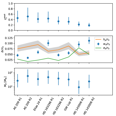
Figure 5: Summary of the numbers resulting from the Gaussian fitting of the radial profiles of the rings, as listed in Table 2. Top: The optical depth of the ring at the peak of the intensity ($\tau_{\nu}^{\mathrm{peak}}$). Middle: The relative size, in units of the ring radius $r_{0}$, of the dust ring width $w_{d}$, the pressure scale height $h_{p}$ and the standard deviation beam size $\sigma_{b}$.

5 The rings as dust traps

The hypothesis we are now going to test is that the rings are caused by dust trapping in axisymmetric pressure bumps. For simplicity we will assume that the radial gas pressure profile is fixed in time, and there is no back-reaction of the dust onto the gas. The pressure bump is assumed to be so strong that the dust trapping in these rings is perfect: no dust escapes. We then expect that the dust distribution finds an equilibrium between dust drift and turbulent spreading.

5.1 Model

Consider the following radial Gaussian profile for the pressure at the disk midplane:

$$p(r)=p_{0}\exp\left(-\frac{(r-r_{0})^{2}}{2w^{2}}\right)$$ (13)

where $w$ is the width, and $p_{0}$ is the pressure at the peak of the pressure bump, located at $r=r_{0}$. The width has to obey $w\geq h_{p}$ to ensure stability (see Appendix G).

The equilibrium between radial drift and radial mixing leads to the following radial distribution of the dust (see Appendix F for the derivation):

$$\Sigma_{\mathrm{d}}(r)=\Sigma_{\mathrm{d0}}\exp\left(-\frac{(r-r_{0})^{2}}{2w_{\mathrm{d}}^{2}}\right)$$ (14)

where

$$w_{\mathrm{d}}=w\,\left(1+\psi^{-2}\right)^{-1/2}$$ (15)

with $\psi$ given by

$$\psi=\sqrt{\frac{\alpha_{\mathrm{turb}}}{\mathrm{Sc}\,\mathrm{St}}}$$ (16)

Here $\mathrm{St}$ is the Stokes number of the dust particles (Eq. F3), $\mathrm{Sc}$ is the Schmidt number of the turbulence in the gas (the ratio between turbulent viscosity and turbulent diffussivity), and $\alpha_{\mathrm{turb}}$ is the usual turbulence parameter. Note that this solution is for a single grain size.

For large grains and/or weak turbulence one finds $\psi\ll 1$, which leads to $w_{\mathrm{d}}\ll w$. In this case the dust is strongly trapped near the peak of the pressure bump. The opposite is the case for small grains and/or strong turbulence, for which one gets $\psi\gg 1$, which leads to $w_{\mathrm{d}}\rightarrow w$. In this case the trapping is very weak and the dust-to-gas ratio within the pressure bump stays nearly constant.

It is interesting to note that this parameter $\psi$ also determines the degree of vertical settling of the same dust:

$$h_{\mathrm{d}}=h_{p}\,\left(1+\psi^{-2}\right)^{-1/2}$$ (17)

In other words: dust particles that are radially trapped in a narrow ring are also vertically settled. This does not mean, however, that dust that is not settled can always radially drift through any dust trap. In fact: even for $\psi\gg 1$ our model still assumes that all the dust remains trapped, albeit in the far wings of the Gaussian pressure trap. This has relevance for dust trapping in the edges of planetary gaps, which we will discuss in Section 6.

Eq. (14) has only three parameters: $\Sigma_{\mathrm{d0}}$, $w_{\mathrm{d}}$ and $r_{0}$. As we have shown in Sections 3, 4.1 and 4.2, all three parameters can be extracted from the observations. The main uncertainty lies in $\Sigma_{\mathrm{d0}}$, due to the uncertainty in the dust opacity. The values of $w_{\mathrm{d}}$ for the rings in our sample can be directly taken from Table 2.

The width of the dust ring $w_{\mathrm{d}}$ is physically set by $\alpha_{\mathrm{turb}}$, $\mathrm{Sc}$, $\mathrm{St}$ and $w$ through the above equations. We therefore have one observational value for four unknown parameters. This is heavily degenerate. All we can do is to test if the measured value of $w_{\mathrm{d}}$ is consistent with expected values of $\alpha_{\mathrm{turb}}$, $\mathrm{Sc}$, $\mathrm{St}$ and $w$.

5.2 Limits to $\alpha_{\mathrm{turb}}$, $\mathrm{Sc}$, $\mathrm{St}$ and $w$

Reasonable values of $\alpha_{\mathrm{turb}}$, $\mathrm{Sc}$, $\mathrm{St}$ and $w$ obey certain restrictions. First of all, the Schmidt number $\mathrm{Sc}$ is merely a way to relate the turbulent viscosity with the turbulent mixing. If we do not strive to learn about the turbulent viscosity, and instead are satisfied with learning only about the turbulent mixing, then we are only interested in the combination $\alpha_{\mathrm{turb}}/\mathrm{Sc}$. For simplicity we set $\mathrm{Sc}=1$, which is a reasonable value (Johansen & Klahr, 2005).

The value of the turbulence parameter $\alpha_{\mathrm{turb}}$ is usually considered to be between $10^{-6}\lesssim\alpha_{\mathrm{turb}}\lesssim 10^{-2}$.

The width of the pressure bump cannot be smaller than about a pressure scale height, but also not smaller than the width of the dust ring. Therefore $w_{\mathrm{min}}=\mathrm{max}(h_{p},w_{\mathrm{d}})$. In the case of the double rings (AS 209, HD 163296 and HD 143006), the full-width-at-half-maximum $2.355\,w$ should not exceed the radial separation of the rings. For the two single ring sources we take the distance from the peak to the deepest point of the gap to the inside of the ring as the upper limit on the half-width-at-half-maximum $1.178\,w$. These lower and upper limits on $w$ are listed in Table 3.

The Stokes number $\mathrm{St}$ can be any value. But it is directly related to the grain size $a$ and the gas density $\rho_{\mathrm{g}}$, where the gas density is directly related to the gas surface density $\Sigma_{\mathrm{g}}$ via $\Sigma_{\mathrm{g}}=\sqrt{2\pi}h_{p}\rho_{\mathrm{g}}$. If we have observational constraints on the grain size $a_{\mathrm{grain}}$ and a good estimate of the gas surface density $\Sigma_{\mathrm{g}}$, then we can eliminate this uncertainty, and we are left with two unknown parameters ($\alpha_{\mathrm{turb}}$ and $w$) for one measurement ($w_{\mathrm{d}}$). Unfortunately, while estimating $a_{\mathrm{grain}}$ from observations may be doable, it is far more difficult to estimate $\Sigma_{\mathrm{g}}$. Standard disk gas mass estimates are of limited use, as they are based on measuring the dust mass and multiplying it by the estimated gas-to-dust ratio. Since we are testing the hypothesis of dust trapping, we cannot assume a standard gas-to-dust ratio.

One can, however, set an upper bound on $\Sigma_{\mathrm{g}}$ by demanding that the disk is gravitationally stable, i.e. that the Toomre parameter obeys

$$Q_{\mathrm{Toomre}}\equiv\frac{c_{s}\Omega_{K}}{\pi G\Sigma_{\mathrm{g}}}>2$$ (18)

Otherwise non-axisymmetric features, such as spiral arms, would develop (see e.g. Kratter & Lodato, 2016), which would also be seen in the continuum emission. Here $c_{s}=\sqrt{k_{B}T_{\mathrm{g}}/\mu m_{p}}$ is the isothermal sound speed (with $T_{\mathrm{g}}$ being the gas temperature), $\Omega_{K}=\sqrt{GM_{*}/r^{3}}$ is the Kepler frequency, $G$ is the gravitational constant, and $\Sigma_{\mathrm{g}}$ the gas surface density. Taking the disk midplane temperature from Table 2, which was calculated using Eq. (5), we can compute the upper limits on $\Sigma_{\mathrm{g}}$ for all of the rings. The results are listed in Table 3 as $\Sigma_{\mathrm{g,max}}$.

Table 3: Limits on the free parameters of the dust trapping model.

Source	Ring	Name	$w_{\mathrm{min}}$	$w_{\mathrm{max}}$	$\Sigma_{\mathrm{g,min}}$	$\Sigma_{\mathrm{g,max}}$	$a_{\mathrm{max}}$	$\mathrm{St}_{(a=0.02\,\mathrm{cm})}$	$w_{d}/w$	$\alpha/\mathrm{St}$	$\alpha/\mathrm{St}$	$\alpha_{\mathrm{exmp}}$
			$[\mathrm{au}]$	$[\mathrm{au}]$	$[\mathrm{g}/\mathrm{cm}^{2}]$	$[\mathrm{g}/\mathrm{cm}^{2}]$	$[\mathrm{cm}]$	(for $\Sigma_{\mathrm{g,max}}$)	(for $w_{\mathrm{max}}$)	(for $w_{\mathrm{max}}$)	(for $w_{\mathrm{min}}$)
(1)	(2)	(3)	(4)	(5)	(6)	(7)	(8)	(9)	(10)	(11)	(12)	(13)
AS 209	1	B74	5.6	19.6	2.3e-01	1.6e+01	4.7	3.2e-03	0.17	3.1e-02	5.7e-01	9.9e-05
AS 209	2	B120	10.3	19.6	2.6e-01	6.9e+00	1.2	7.6e-03	0.21	4.6e-02	1.9e-01	3.5e-04
Elias 24	1	B77	7.2	17.1	2.1e-01	1.8e+01	5.8	3.0e-03	0.27	7.7e-02	6.6e-01	2.3e-04
HD 163296	1	B67	6.8∗	13.8	2.2e-01	4.0e+01	15.4	1.3e-03	0.50	3.3e-01	–	4.2e-04
HD 163296	2	B100	7.1	13.8	1.7e-01	2.0e+01	9.5	2.6e-03	0.34	1.3e-01	7.7e-01	3.3e-04
GW Lup	1	B85	7.5	9.9	1.6e-01	7.8e+00	2.7	6.7e-03	0.48	3.1e-01	6.8e-01	2.1e-03
HD 143006	1	B41	3.9∗	10.1	1.1e-01	7.5e+01	60.6	7.0e-04	0.39	1.8e-01	–	1.2e-04
HD 143006	2	B65	7.3∗	10.1	9.4e-02	3.4e+01	30.8	1.6e-03	0.72	1.1e+00	–	1.7e-03

Note. — Columns 1 to 3 are the same as in Table 2. (4) Lower limit to the pressure bump width $w_{\mathrm{min}}$ (for $w_{d}\leq h_{p}$ this is $h_{p}$; for $w_{d}>h_{p}$, marked with the symbol ^∗, this is $w_{d}$). (5) Upper limit to the pressure bump width $w_{\mathrm{max}}$, derived from the separation between the rings (for AS 209, HD 163296 and HD 143006) or from the separation of the ring to the nearest minimum (for Elias 24 and GW Lup). (6) Lower limit on the gas surface density $\Sigma_{\mathrm{g}}$ derived by demanding $\Sigma_{\mathrm{g}}\gtrsim\Sigma_{\mathrm{d}}$. Note that this involves the uncertainty in $\Sigma_{\mathrm{d}}$ due to the uncertainty of the dust opacity model. (7) Upper limit on the gas surface density derived from demanding that the gas disk is gravitationally stable. (8) Maximum grain size $a_{\mathrm{max}}$ for which the derived dust surface density (based on the DSHARP opacity model) together with the gas surface density remain gravitationally stable. (9) Example value of the Stokes number $\mathrm{St}$ for grains with a radius of $0.02\,\mathrm{cm}$. (10) Estimate of the degree of dust trapping given by the ratio $w_{d}/w$ (assuming that $w=w_{\mathrm{max}}$). The smaller this number is, the stronger the dust trapping. (11) Value of $\alpha/\mathrm{St}$ derived for the widest gas bump. (12) Value of $\alpha/\mathrm{St}$ derived for the narrowest gas bump. (13) Example value of $\alpha_{\mathrm{turb}}$, computed for $w=w_{\mathrm{max}}$, $\Sigma_{\mathrm{g}}=\Sigma_{\mathrm{g,max}}$ and $a=0.02\,\mathrm{cm}$.

One can estimate a lower limit to the gas density by demanding that the gas surface density must be at least as large as the dust surface density, since dust trapping is unlikely to achieve a larger concentration of dust than that. For the dust surface density we use Eq. (12) at $r=r_{0}$, with $\tau_{\nu}(r_{0})=\tau_{\nu}^{\mathrm{peak}}$ from Table 2. By demanding that

$$\Sigma_{\mathrm{g}}\gtrsim\Sigma_{\mathrm{d}}(r_{0})=\frac{\tau_{\nu}^{\mathrm{peak}}}{\kappa_{\nu}^{\mathrm{abs}}}$$ (19)

and using our standard opacity of $\kappa_{\nu}^{\mathrm{abs}}=2.0{}\,\mathrm{cm}^{2}/\mathrm{g}$ we arrive at values for $\Sigma_{\mathrm{g,min}}(r=r_{0})$ listed in Table 3 as $\Sigma_{\mathrm{g,min}}$.

It is likely that even for larger values of the gas surface density the dust-gas mixture becomes unstable to the streaming instability and other types of instabilities, because the dust will likely settle to the midplane, increasing the ratio $\rho_{\mathrm{d}}/\rho_{\mathrm{g}}$. We can quantify this. For a given ratio $\alpha_{\mathrm{turb}}/\mathrm{St}$, we can compute the ratio $h_{d}/h_{p}$ from Eqs. (16, 17), which tells us how strongly the dust is settled. The new (and more stringent) lower limit to the gas density is then $\Sigma_{\mathrm{g,min}}^{\mathrm{sett}}=(h_{p}/h_{d})\,\Sigma_{\mathrm{g,min}}$.

If the grains are much larger than $\lambda/(2\pi)\simeq 0.02\,\mathrm{cm}$, the opacity drops and the resulting dust surface density estimate increases, also yielding larger values of $\Sigma_{\mathrm{g,min}}$. Along this line of thinking one can compute the largest grain radius for which $\Sigma_{\mathrm{g,min}}<\Sigma_{\mathrm{g,max}}$, i.e. for which the $\Sigma_{\mathrm{g,min}}$ is consistent with $Q_{\mathrm{Toomre}}>2$. This gives a lower limit to the dust opacity $\kappa_{\nu}^{\mathrm{abs}}$ and, as a result, an upper limit to the grain size. Given that the total surface density is then twice the gas surface density (the dust contributing the other half), we have to introduce a factor of 2. The condition on the opacity is then:

$$\kappa_{\nu}^{\mathrm{abs}}\gtrsim\frac{2\tau_{\nu}^{\mathrm{peak}}}{\Sigma_{\mathrm{g,max}}}$$ (20)

We now use the DSHARP opacity model (Birnstiel, 2018) to translate this $\kappa_{\nu}^{\mathrm{abs}}$ into a grain radius. We arrive at values of centimeters to half a meter (Table 3). These are conservative limits, with real values likely to be substantially smaller. Indeed, in the next Subsection we will derive, from the values of $\alpha_{\mathrm{turb}}/\mathrm{St}$ in Table 3, much more stringent upper limits on the grain size.

5.3 Application to the observed rings

We now apply the model of Subsection 5.1 with the limits on the parameter ranges derived in Subsection 5.2 to the observed ring widths $w_{d}$ listed in Table 2. The goal is to see which constraints the observations can put on the physics of the observed rings of this paper.

From an assumed value of $w$ and the measured value $w_{\mathrm{d}}$ we can directly compute the ratio $\alpha_{\mathrm{turb}}/\mathrm{St}$

$$\frac{\alpha_{\mathrm{turb}}}{\mathrm{St}}\equiv\psi^{2}=\left[\left(\frac{w}{w_{\mathrm{d}}}\right)^{2}-1\right]^{-1}$$ (21)

where we used Eqs. (15, 16), and set $\mathrm{Sc}=1$. We will consider two choices of $w$: the $w_{\mathrm{min}}$ and $w_{\mathrm{max}}$ from Table 3.

For the choice $w=w_{\mathrm{max}}$ (the widest possible pressure bump) the dust rings are all narrower than the gas rings: $w_{\mathrm{d}}<w$, as can be seen from the $w_{d}/w$ column in Table 3. This implies that, under the assumption that $w=w_{\mathrm{max}}$, the dust trapping is operational. The ratio $w_{d}/w$ gives an indication of the degree of dust trapping: the smaller this value is, the closer the dust has drifted to the peak of the pressure bump before turbulent mixing halts further narrowing of the dust ring. The strength of the turbulence for this case is given by the $\alpha_{\mathrm{turb}}/\mathrm{St}$ column for $w=w_{\mathrm{max}}$ in Table 3.

One important result from this analysis is that, although these rings are the narrowest that have been observed so far, the ratio $w_{d}/w$ is never smaller than 17%, usually subtantially larger. This means that in all these rings turbulence prevents the dust from forming even narrower dust rings. Perhaps this is self-induced turbulence due to the large $\Sigma_{d}/\Sigma_{g}$ ratio in this dust trap. Or it could mean that the dust is still not yet in drift-mixing equilibrium, which would require the grains to be very small (i.e. have a very low value of $\mathrm{St}$). In Section 6 we will discuss an example of the latter scenario.

For the choice $w=w_{\mathrm{min}}$ (the narrowest possible pressure bump) we can only use Eq. (21) for the rings for which $w_{\mathrm{d}}<h_{p}$. The reason is that for those rings with $w_{\mathrm{d}}>h_{p}$ (marked with a ^∗ in Table 3) the minimal pressure bump width is $w_{\mathrm{min}}=w_{\mathrm{d}}$, and the dust ring is as wide as the pressure bump, implying that dust trapping is weak or non-operational. Any increase of $\alpha_{\mathrm{turb}}/\mathrm{St}$ will keep $w_{\mathrm{d}}=w_{\mathrm{min}}$, so one cannot derive any value for $\alpha_{\mathrm{turb}}/\mathrm{St}$. But for other rings (those not marked with *) we can compute $\alpha_{\mathrm{turb}}/\mathrm{St}$. The resulting values for both choices of pressure bump width are given in Table 3, columns 11 and 12. They can be understood as the lower and upper limit on $\alpha_{\mathrm{turb}}/\mathrm{St}$.

We conclude that for those rings not marked with the ${*}$-symbol in Table 3, our data is clear proof of dust trapping occurring. For the rings marked with $*$ the narrowness of the dust ring can also be explained simply by the narrowness of the underlying gas ring without the need for dust trapping, although it does not exclude dust trapping either.

The next task is to convert from Stokes number $\mathrm{St}$ to grain radius $a_{\mathrm{grain}}$. The Epstein regime is valid for grain sizes of the order of millimeters or centimeters, in which case $a_{\mathrm{grain}}$ and $\mathrm{St}$ are related by

$$\mathrm{St}=\frac{\pi}{2}\frac{\xi_{\mathrm{dust}}a_{\mathrm{grain}}}{\Sigma_{\mathrm{g}}}$$ (22)

where $\Sigma_{\mathrm{g}}$ is the gas surface density and $\xi_{\mathrm{dust}}$ is the material density of the dust grains. For the DSHARP opacity model (Birnstiel, 2018) the average material density of the dust aggregates is $\xi_{\mathrm{dust}}\simeq 1.67{}\,\mathrm{g}/\mathrm{cm}^{3}$.

To get a feeling for the results, let us choose the grain size to be $a_{\mathrm{grain}}=0.02\,\mathrm{cm}$, which corresponds to $\lambda/2\pi$ for $\lambda=0.125\,\mathrm{cm}$ (the wavelength of ALMA band 6). The corresponding Stokes numbers, for the most massive possible gas disk ($\Sigma_{\mathrm{g}}=\Sigma_{\mathrm{g,max}}$), are listed in Table 3, column 9. This then allows us to convert the value of $\alpha_{\mathrm{turb}}/\mathrm{St}$ into a value of $\alpha_{\mathrm{turb}}$, which we shall call $\alpha_{\mathrm{exmp}}$, indicating that it is an example value for a particular choice of $a_{\mathrm{grain}}$. For the case $w=w_{\mathrm{max}}$ this leads to values $\alpha_{\mathrm{exmp}}=10^{-4}\ldots\mathrm{few}\,\times 10^{-3}$, listed in Table 3, column 13.

These low values of $\alpha_{\mathrm{turb}}$ are consistent with the low values or upper limits reported recently (Pinte et al., 2016; Flaherty et al., 2018). However, it has to be kept in mind that the values of $\alpha_{\mathrm{turb}}=\alpha_{\mathrm{exmp}}$ were derived for an extremal choice of parameters: $w=w_{\mathrm{max}}$, $\Sigma_{\mathrm{g}}=\Sigma_{\mathrm{g,max}}$, and only for grain radius $a=0.02\,\mathrm{cm}$. For a smaller value of $w$, a lower value of $\Sigma_{\mathrm{g}}$, or larger grains, the computed value of $\alpha_{\mathrm{turb}}$ will increase. If we take ring 1 of AS 209 as an example, and take $w=w_{\mathrm{min}}$, we see from Table 3 that $\alpha/\mathrm{St}=0.57$. Using $\Sigma_{\mathrm{g}}=\Sigma_{\mathrm{g,min}}$ (but keep $a_{\mathrm{grain}}=0.02\,\mathrm{cm}$) we get $\mathrm{St}=0.23$ from Eq. (22), yielding $\alpha_{\mathrm{turb}}=0.13$. This is much higher than the value of $\alpha_{\mathrm{exmp}}$, and it demonstrates that it is hard to set a true upper limit on $\alpha_{\mathrm{turb}}$ from these observations.

Can we derive a lower limit to $\alpha_{\mathrm{turb}}$? This depends on whether we have information about the grain size. The value of $\alpha_{\mathrm{exmp}}$ is the smallest possible value of $\alpha_{\mathrm{turb}}$ consistent with the data, for an assumed grain size of $a=0.02\,\mathrm{cm}$. Since Eq. (22) shows that $a_{\mathrm{grain}}$ and $\mathrm{St}$ are linearly related, we can generalize this to the smallest possible value of $\alpha_{\mathrm{turb}}$ consistent with the data, for any given grain size $a_{\mathrm{grain}}$:

$$\alpha_{\mathrm{turb}}\geq\left(\frac{a_{\mathrm{grain}}}{0.02\,\mathrm{cm}}\right)\;\alpha_{\mathrm{exmp}}$$ (23)

With the values of $\alpha_{\mathrm{exmp}}$ listed in Table 3 this shows that, even for disks so massive that they are nearly gravitationally unstable, we can exclude the combination of very low $\alpha_{\mathrm{turb}}\ll 5\times 10^{-4}$ and very large grains $a_{\mathrm{grain}}\gg 0.1\,\mathrm{cm}$ for all the rings of our sample. In many of the rings this constraint is much more strict (i.e. toward smaller grains and/or stronger turbulence).

To obtain estimates of the grain size we need spectral information. At present we have only the high resolution data for band 6, so we do not yet have information about the radial profile of the spectral slope. But in several recent observations of the spectral index across ringed disks (ALMA Partnership et al., 2015; Tsukagoshi et al., 2016; Huang et al., 2018) one clearly sees that $\alpha_{\mathrm{spec}}$ varies across these rings, being closer to $2$ at the ring center and substantially larger between the rings. This makes sense in terms of the dust trapping scenario in which we expect larger grains to be trapped more efficiently (and thus dominate the peak of the ring) than smaller grains, because the smaller grains will be more subject to turbulent mixing. It is clear that we need such data to be able to constrain $a_{\mathrm{grain}}$, and then, via Eq. (23), set limits on the turbulence.

5.4 Including a grain size distribution

So far we have only looked at a single grain size, for which the solution is a Gaussian radial grain distribution centered around the point of zero gas pressure gradient. The model fits fairly well the near-Gaussian profiles that we observe. However, in several rings we find a deviation from Gauss in the form of an excess emission in the wings of the profile. Could this be a result of a grain size distribution? To find out, let us apply our model to the following powerlaw size distribution:

$$m(a)\frac{dN}{d\ln a}=\frac{dM}{d\ln a}\propto a^{p}$$ (24)

where $a$ is the grain size, $m(a)$ the corresponding grain mass, $N$ the cumulative particle number and $M$ the cumulative dust mass. The parameter $p$ is the size distribution powerlaw coefficient, and it is $p=1/2$ for the usual MRN distribution (this corresponds to $dN/da\propto a^{p-4}=a^{-3.5}$). We also need to define limits $a_{\mathrm{min}}$ and $a_{\mathrm{max}}$. The radial surface density solution, Eq. (F9), then becomes:

$$\frac{d\Sigma_{\mathrm{d}}(r)}{d\ln a}=\frac{1}{(2\pi)^{3/2}r_{0}w_{\mathrm{d}}(a)}\frac{dM}{d\ln a}\exp\left(-\frac{(r-r_{0})^{2}}{2w_{\mathrm{d}}(a)^{2}}\right)$$ (25)

At each radius $r$ the local size distribution is different from other radii, with larger grains dominating near $r=r_{0}$ and smaller grains dominating in the wings.

To demonstrate the effect we will try to apply this multi-size dust trapping model to ring 1 of AS 209. We set the gas ring width to $w=19.6\,\mathrm{au}$, and gas surface density to $\Sigma_{g}=16\,\mathrm{g}\,\mathrm{cm}^{-2}$, i.e. the maximum $w$ and $\Sigma_{g}$ as listed in Table 3. We set $\alpha_{\mathrm{turb}}=1.1\times 10^{-3}$, $p=1/2$ (MRN slope), $a_{\mathrm{min}}=10^{-2}\,\mathrm{cm}$ and $a_{\mathrm{max}}=1\,\mathrm{cm}$. We take 10 grain size bins logarithmically spaced in $a$. For the rest we take the same parameters as listed in Table 2. Since the relation between the observed emission and the underlying dust mass is different if we take a size distribution, we adjust the dust mass such that the model yields a peak optical depth equal to the $\tau_{\nu}^{\mathrm{peak}}$ value from Table 2. We use the DSHARP opacities, which vary strongly over the grain size range $[a_{\mathrm{min}},a_{\mathrm{max}}]$ we take.

The total optical depth profile of this model is shown in Fig. 6. To see if this profile displays excess emission in the wings, we fitted a Gaussian to the core of the profile, in the same manner as we did in Section 3. We find indeed that the core behaves nicely as a Gaussian, while the wings have excess, as expected. The total required dust mass increases to 110 $M_{\oplus}$.

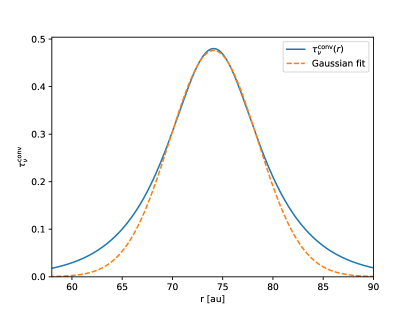
Figure 6: Total optical depth profile of the dust trapping model with a size distribution (solid line). The dashed line shows the Gauss curve that best fits the core of the profile.

However, the model is symmetric, so it cannot explain the asymmetric excess of most rings. Some rings even show excess only on one side. In Section 6 we will address another scenario for the excess emission, which can explain also the asymmetry.

The most important results we obtained in this section are summarized in Fig. 7.

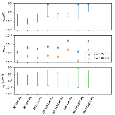
Figure 7: Summary of the numbers resulting from the Gaussian dust trapping model analysis, as listed in Table 3. Top: The values of $\alpha_{\mathrm{turb}}/\mathrm{St}$ found for the rings. Middle: The values of $\alpha_{\mathrm{turb}}/a_{\mathrm{grain}}$ for two choices of grain size, for the choice of $w=w_{\mathrm{max}}$ (leading to lowest possible values of $\alpha_{\mathrm{turb}}/a_{\mathrm{grain}}$). Bottom: Inferred range of gas surface density (bottom limit: $\Sigma_{g}\geq\Sigma_{d}$, top limit: gravitational instability).

6 Planet gaps as dust traps and deviations from Gaussian shape

So far our models of dust trapping were quite idealized, in particular the assumption of a gaussian pressure bump. In reality the radial pressure profile is presumably better described by a smooth background profile with perturbations imposed on it. The background profile could be, for instance, a powerlaw like $p(r)\propto r^{-k}$ with index $k$ being $k=-2.5$. The perturbation could then be a pressure bump or a pressure dip, the latter being the case for a planetary gap. Given that the overall background pressure declines with increasing $r$, such a dip/gap, if strong enough, could lead to a local pressure maximum at the outer edge of the gap. That would then be where the dust gets trapped (e.g. Rice et al., 2006; Zhu et al., 2012; Pinilla et al., 2012a). This pressure maximum would then not be symmetric like the Gaussian pressure bump model of Section 5, but instead is likely to be shallower on the outside and steeper on the inside.

As we know from the analysis of Section 5, the widths of the dust rings of our sample are, in most cases, not very much narrower than the widths of the gas pressure bumps (see $w_{d}/w$ column in Table 3). That means that the deviation of the gas pressure bump from a Gaussian profile may affect the shape of the dust ring profile too. If $w_{d}/w$ were to be very small, the dust is only sensitive to the very peak of the pressure bump profile. The larger $w_{d}/w$ is, the more the dust “feels” any non-Gaussian deviations in the wings of the bump. For AS 209, with $w_{d}/w$ of the order of 0.2 for both rings (for the choice $w=w_{\mathrm{max}}$, see Table 3, column 10), we thus expect the dust ring profiles to be closer to Gaussian shape (modulo grain size distribution effects) than for HD 163296, for example.

The question is: what do the wing-excesses in our ring sample tell us about the shape of the underlying pressure bump? And can we learn about its origin?

Rather than addressing this question in a very general manner, we will start straight from the scenario of a gap-opening planet. In another paper of this series (Zhang, 2018), this hypothesis is investigated with detailed hydrodynamic simulations of planet-disk interaction. Here, instead, we will reduce this hypothesis to a very rudimentary model: a Gaussian dip in an otherwise smoothly declining pressure profile. This produces an asymmetric pressure bump at the outer edge of the gap.

The problem is now no longer a local one, but a global one: all the dust beyond the gap may, in time, drift into the dust trap and add to its mass. We are forced to leave analytical modeling behind and employ numerical techniques.

Our model is a 1-D viscous disk evolution model with a single dust component added, which can radially drift and will be prone to radial turbulent mixing. The equations of this model are standard, and have been repeated numerous times in the literature (e.g. Adachi et al., 1976; Brauer et al., 2007; Garaud, 2007; Birnstiel et al., 2010; Zhu et al., 2012; Sato et al., 2016). Here we repeat the basic ones. The gas surface density obeys

$$\frac{\partial\Sigma_{g}}{\partial t}+\frac{1}{r}\frac{\partial\left(r\,\Sigma_{g}\,v_{gr}\right)}{\partial r}=0$$ (26)

with the radial gas velocity $v_{gr}$ given by

$$v_{gr}=-\frac{3}{\Sigma_{g}\sqrt{r}}\frac{\partial(\sqrt{r}\,\Sigma_{g}\nu_{\mathrm{turb}})}{\partial r}$$ (27)

with $\nu_{\mathrm{turb}}=\alpha_{\mathrm{turb}}c_{s}^{2}/\Omega_{K}$ the turbulent viscosity of the disk. The dust surface density obeys

$$\frac{\partial\Sigma_{d}}{\partial t}+\frac{1}{r}\frac{\partial\left(r\,\Sigma_{d}\,v_{dr}\right)}{\partial r}=\frac{1}{r}\frac{\partial}{\partial r}\left[rD\Sigma_{g}\frac{\partial}{\partial r}\left(\frac{\Sigma_{d}}{\Sigma_{g}}\right)\right]$$ (28)

with the radial dust velocity $v_{dr}$ given by

$$v_{dr}=\frac{1}{1+\mathrm{St}^{2}}\,v_{gr}+\frac{1}{\mathrm{St}^{-1}+\mathrm{St}}\frac{c_{s}^{2}}{\Omega_{K}r}\frac{d\ln p}{d\ln r}$$ (29)

and the turbulent diffusion constant $D=\nu_{\mathrm{turb}}/(1+\mathrm{St}^{2})$.

We will show here only a single example model, applied to ring 2 of HD 163296. An extensive study, applied to all the rings of this sample, will be presented in a forthcoming paper. For our example model we set up a disk according to the classic Lynden-Bell & Pringle model (Lynden-Bell & Pringle, 1974; Hartmann et al., 1998) with an initial radius of 100 au, an initial disk mass of $10^{-1}\,M_{\odot}$. The temperature profile follows the flaring angle recipe (Eq. 5) with $\varphi=0.02$ at all times, and the turbulence parameter is set to $\alpha_{\mathrm{turb}}=10^{-2}$. We make a Gaussian dent into the disk model at $r_{p}=85\,\mathrm{au}$ by defining a factor $F(r)$

$$F(r)=\exp\left[-f\exp\left(-\frac{(r-r_{p})^{2}}{2w_{\mathrm{gap}}^{2}}\right)\right]$$ (30)

such that

$$\Sigma_{g}(r)=\Sigma_{g0}(r)\,F(r)$$ (31)

where $\Sigma_{g0}(r)$ is the unperturbed disk. We take the width of the gap to be $w_{\mathrm{gap}}=6\;\mathrm{au}$ and the depth to be $f=2$. If we would viscously evolve the disk without accounting for the continuous gap-opening force by the planet, this initial gap would quickly be closed. To keep the gap open, without having to include the complexities of planet-disk interaction (which anyway would require at least a 2-D analysis), we apply the trick to replace the disk viscosity (but not the turbulent mixing parameter) with

$$\nu_{\mathrm{turb}}(r)=\nu_{\mathrm{turb},0}(r)/F(r)$$ (32)

Now we add the dust with an initial dust-to-gas ratio of $1:100$. As a grain size we take $a_{\mathrm{grain}}=4\times 10^{-3}\,\mathrm{cm}$. We do not include grain growth in this model.

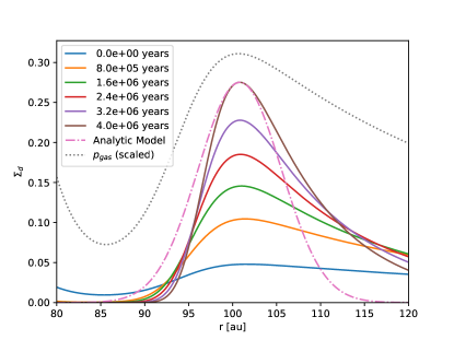
Figure 8: Result of the numerical dust drift model described in Section 6. Shown is the dust surface density of the dust near ring 2 of HD 163296 as it piles up in the pressure bump induced by the gap centered at 85 au. The dotted line shows, in a rescaled manner, the midplane gas pressure profile. The dot-dashed line shows the analytic solution of Section 5, normalized to the final curve of the numerical model.

The results of this model are shown in Fig. 8. One can see that, as expected, the dust drifts into the local pressure peak located at $r_{0}=101\,\mathrm{au}$. As time goes by, more and more dust piles up there. The dust trap essentially collects all the dust from the outer disk regions. At 4 Myr the dust pile-up is still on-going and no steady state is reached yet. This is due to our choice of relatively small dust grains. Had we chosen larger ones, the shape would have more quickly found its equilibrium shape, but it would have been significantly narrower, which is inconsistent with the observed dust ring width of ring 2 of HD 163296.

Overplotted is the analytic solution of Section 5. This solution needs a value of $w$, which we numerically compute from the second derivative of the midplane pressure profile: $w=\sqrt{-p(r_{0})/(d^{2}p(r)/dr^{2})_{r=r_{0}}}$. We see that the width of the numerical profile of the dust surface density is more or less consistent with the analytic result, but its shape is much steeper inside of $r_{0}$, and much shallower outside. This has two causes. One cause is the fact that the pressure profile is not a Gaussian, but is asymmetric. The other is that even at 4 Myr there is still dust flowing into the dust trap, in particular from the outside. The continuing steepening on both sides shows that the influx of dust declines with time, as the dust inside and outside of the bump gets depleted.

This section shows the limitations of the analytic solutions of Section 5. While the overall derived quantities such as the width of the dust ring are fairly well described by the analytic model, the deviations from Gaussian shape may not only be a result of the grain size distribution, but, as we see in this Section, also due to the non-Gaussian shape of the pressure bump and to the fact that the dust has not yet reached an equilibrium state.

Given that the complexity of the numeric model is much higher than our analytic models, we defer a more detailed parameter study and application of this model to the DSHARP sample to a follow-up paper.

7 Discussion

7.1 Why are most rings so “fine-tuned”?

It is rather striking that in the analysis of the rings up to this point we have found several rather “fine-tuned” properties. For instance, the rings in the disks around AS 209, Elias 24, GW Lup and the inner ring in the disk around HD 143006 have a width that is only roughly twice the beam size (between $1.6$ and $2.7$ times, to be precise), but none are unresolved. Given the small sample, and the fact that we selected isolated rings, it is very well possible that this is just coincidence. The fact that some rings (in particular the inner ring of HD 163296) are clearly much wider, lends some support to this.

The derived peak optical depths for most sources (except HD 143006), assuming our model of the dust temperature is correct, hover around 0.4, i.e. just in between the optically thin and optically thick regime. This also appears rather fine-tuned. Part of the explanation could be the fact that we selected the strongest-contrast rings in the DSHARP sample for our analysis. That may explain why none of our rings have very low optical depth. But it does not explain why none of them are very optically thick (flat-topped).

Finally, many of the ring profiles are remarkably similar to a Gaussian shape. This may be due to the fact that the rings are only a few beams wide, which may make non-Gaussian profiles appear more Gaussian after convolution. But it is unclear whether this explanation is sufficient.

We therefore conclude that we do not know for sure whether the “fine-tunedness” of the rings in our sample is a real signal with a physical meaning, or an artifact of some kind. The question is, to which extent this uncertainty could affect our conclusions.

One of the main conclusions of our study is the fact that all the rings in our subsample are spatially resolved, which shows that the dust trapping is not effective enough to produce very thin dust rings with $w_{d}\ll h_{p}$. This is an important conclusion, which is also reflected in the typical values of $\alpha_{\mathrm{turb}}/\mathrm{St}$ we derived (Table 3). Fortunately, this conclusion does not rely only on the measurement of $w_{d}$. It is also supported by a flux argument: The intensity before convolution cannot exceed the Planck function. So assuming that our temperature estimate is correct, the minimal full width $\Delta r$ of the dust ring would then be $\Delta r=\sqrt{2\pi}\sigma A/B_{\nu}(T_{d})$, where the factor $\sqrt{2\pi}$ originates from the integral over the Gauss curve. For ring 1 of AS 209, for instance, this gives a width $\Delta r\simeq 3.36\,\mathrm{au}$. This is about half the FWHM of the current Gauss estimate. In other words: even if, hypothetically, our measurement of the width of the rings is entirely wrong, the fact that the rings are so bright (only about a factor of 2 below the Planck function) shows that the rings cannot be much narrower than the beam.

7.2 Can a resolved ring be in fact a blend of several unresolved rings?

Are the rings we see truly single rings, or could they also be made up of a concentric series of radially unresolved rings that are blended into a single ring due to the beam convolution? It is, of course, hard to answer in general, since we have no observational means to resolve structures of sub-beam size.

But from the perspective of particle trapping by a pressure bump this question can be rigorously answered. A long-lived radial pressure perturbation in a protoplanetary disk cannot be much narrower than about a pressure scale height $h_{p}(r)$ (Ono et al., 2016). A dust ring produced by dust trapping in this pressure bump may become rather narrow, dependent on a variety of parameters, as discussed in Section F. But there can not be more than a single such dust ring in each pressure bump.

For the wide rings of HD 163296, even under the most optimistically low disk temperature (e.g. 10 K) the pressure scale height at rings 1 and 2 are 2.4 au and 4.3 au, respectively, which correspond to FWHM widths of 55 and 101 milliarcseconds, respectively. Clearly the ALMA observations in band 6, with FWHM beam size of 51 mas, spatially resolve the pressure scale height. This means that the ring separation will be spatially resolved by ALMA, ruling out the possibility that the wide rings are made up of a multitude of narrow rings, at least in the dust trapping scenario.

However, the rings may be made up of many unresolved clumps, such as those produced by the streaming instability. Whether the presence of such clumpy structure has observable consequences, in spite of the clumps being spatially unresolved, is an issue that requires deeper study. But one may speculate that the self-regulation mechanism of the streaming instability, as discussed above, may also lead to a self-regulation of the optical depth or, equivalently, the covering fraction of unresolved optically thick clumps.

7.3 Condition for the streaming instability

The “streaming instability” and related processes (Youdin & Goodman, 2005; Johansen & Youdin, 2007; Bai & Stone, 2010; Kowalik et al., 2013; Schäfer et al., 2017; Schreiber & Klahr, 2018) play a fundamental role in the theory of planet formation. Dust traps may be ideal places for this process to operate, because in those regions one can expect the local dust-to-gas ratio to be strongly enhanced over the background. There is the concern that at the precise location of the pressure maximum the streaming instability is killed because the gas orbits exactly with Kepler velocity there. But slightly adjacent to the pressure peak the deviation from Keplerian motion is strong, and may drive such an instability. To keep dust in those adjacent regions, turbulence is required to counteract the trapping. If this turbulence is caused by the streaming instability itself, this is a bit of a “chicken-or-egg” issue. Auffinger & Laibe (2018) report a linear stability analysis that indicates that the streaming instability can occur in pressure bumps. Raettig et al. (2015) present simulations of particle trapping and streaming instability in a vortex, which is in many ways similar to the dust traps we study in this paper. But the final word on this matter has not yet been said. Let us, for the purpose of the argument, assume that the streaming instability, and the related process of gravoturbulent planetesimal formation (Johansen et al., 2007), can indeed occur in a pressure bump.

In the literature it is often mentioned that the streaming instability requires a dust-to-gas surface density ratio of $\Sigma_{\mathrm{d}}/\Sigma_{\mathrm{g}}\gtrsim 0.02$ or higher to operate (Bai & Stone, 2010). This can, however, not be directly compared to our models, because this value of $0.02$ was found for models without any pre-determined turbulence. The turbulence in those models was induced by the streaming instability itself. In our analytic model, on the other hand, we set the turbulence strength by hand, by setting $\alpha_{\mathrm{turb}}$ to some value. In essence, we assume that there is another source of turbulence, such as the magnetorotational instability or the vertical shear instability, that determines the mixing of the dust in the disk (see e.g. Lyra & Umurhan, 2018).

According to Youdin & Goodman (2005) the true criterion for the onset of the streaming instability is the ratio of dust and gas volume densities $\rho_{\mathrm{d}}/\rho_{\mathrm{g}}\gtrsim 1$. The midplane volume density ratio for a single grain species with midplane Stokes number $\mathrm{St}\ll 1$, and given surface density ratio $\Sigma_{\mathrm{d}}/\Sigma_{\mathrm{g}}$, depends on the turbulent strength as

$$\frac{\rho_{\mathrm{d}}}{\rho_{\mathrm{g}}}\simeq\left(1+\frac{\mathrm{St}}{\alpha_{\mathrm{turb}}}\right)^{1/2}\frac{\Sigma_{\mathrm{d}}}{\Sigma_{\mathrm{g}}}$$ (33)

(see Eq. 17, and setting $\mathrm{Sc}=1$). The criterion of $\Sigma_{\mathrm{d}}/\Sigma_{\mathrm{g}}\gtrsim 0.02$ mentioned in the literature thus relates to the criterion $\rho_{\mathrm{d}}/\rho_{\mathrm{g}}\gtrsim 1$ via the turbulent strength and the Stokes number. Given that we do not compute the turbulent strength, but prescribe it, we should rely on the more fundamental volume density criterion of Youdin & Goodman (2005) to assess whether the dust in our model triggers the streaming instability or not.

To get some numbers, let us take ring 1 of AS 209. Let us assume the widest possible pressure bump, i.e. $w=w_{\mathrm{max}}$, for which the ratios $\alpha_{\mathrm{turb}}/\mathrm{St}=3.1\times 10^{-2}$, as listed in Table 3. This leads, with Eq. (33), to a dust-to-gas volume density ratio that is 5.8 times larger than the dust-to-gas surface density ratio. This means that the criterion by Youdin & Goodman (2005) is triggered if $\Sigma_{\mathrm{d}}/\Sigma_{\mathrm{g}}\gtrsim 0.17$. Given that $\Sigma_{\mathrm{d}}=\Sigma_{\mathrm{g,min}}$ (by definition of the latter), we can look up its value in Table 3 and find that for $\Sigma_{\mathrm{g}}\lesssim 1.4\,\mathrm{g}\,\mathrm{cm}^{-2}$ the streaming instability will be triggered. Given that the disk becomes gravitationally unstable for $\Sigma_{\mathrm{g}}\gtrsim 16\,\mathrm{g}\,\mathrm{cm}^{-2}$, this leaves only little more than a factor of 10 room for $\Sigma_{\mathrm{g}}$ to avoid either the streaming instability or the gravitational instability. Note that if we take a narrower pressure bump (e.g. $w=w_{\mathrm{min}}$), the ratio $\alpha_{\mathrm{turb}}/\mathrm{St}$ increases, making it harder for the streaming instability to set in.

In the end we cannot, therefore, say with any certainty whether the streaming instability is operating in these rings or not. But we do find that the likelihood that the conditions are triggered are realistic. The rings we see may therefore consist of unresolved clumps, in which planetesimals may form (Johansen et al., 2007).

However, one may then wonder why this does not immediately convert all dust into planetesimals. This may be due to a self-regulation effect: once a certain fraction of the dust is converted into planetesimals, the remaining dust is no longer dense enough to trigger strong enough clumping (Drążkowska & Dullemond, 2014).

7.4 Caveats of the models

This paper is meant as the initial step of a bottom-up investigation of the ringlike structures found in the DSHARP campaign: starting with the simplest analytic estimates, and building up the complexity and realism of the models, so that is becomes clearer what the data tell us – and what not.

Among the important aspects we have not treated in this paper are: the dust back-reaction onto the gas (e.g. Johansen & Youdin, 2007; Gonzalez et al., 2017; Kanagawa et al., 2017b), the origin of the pressure bumps and/or gaps (e.g. Pinilla et al., 2012a; Béthune et al., 2016; Takahashi & Inutsuka, 2016; Dullemond & Penzlin, 2018), the detailed shape of planetary gaps (e.g. Kanagawa et al., 2017a; Zhang, 2018), 2-D and 3-D effects, full radiative transfer (e.g. Bitsch et al., 2013; Flock et al., 2013), dust growth and fragmentation (e.g. Birnstiel et al., 2010; Okuzumi et al., 2012), and many other things.

Also, if we would include, for the analytic models of the dust traps, a temperature gradient and a background density gradient, the results may be affected. In particular the exact location of the pressure peak may shift.

This paper is therefore not meant to give definitive numbers or conclusions. Rather, it is meant as a starting point of more complex modeling campaigns. One such more complex modeling campaign is the hydrodynamic planet-disk interaction paper by Zhang (2018).

8 Conclusions

We studied the radial structure of the eight most prominent dust rings from the DSHARP sample, and investigated to which extent they are consistent with, and/or indications of, being dust traps.

We can summarize our conclusions as follows:

1. For the rings in AS 209, Elias 24, the outer ring of HD 163296, and the ring of GW Lup the width is narrower than the estimated pressure scale height. This is strong evidence for dust trapping being at work.

2. For none of the 8 rings studied in this paper we found evidence against dust trapping.

3. The dust trapping may explain their longevity, given the fact that dust grains tend to drift into the star on a short time scale in the absense of dust traps (Pinilla et al., 2012b).

4. All rings are radially resolved, by factors $\sigma/\sigma_{b}$ ranging from 1.6 (ring B41 of HD 143006) to 3.2 (ring B67 of HD 163296). When comparing the implied width of the dust ring $w_{d}$ to the largest plausible width of the gas pressure bump $w$, we find that the strongest dust trapping occurs in AS 209, with $w_{d}/w$ ratios of 0.17 and 0.21 for rings 1 and 2, respectively. For the other rings we find larger $w_{d}/w$ values. This indicates that turbulent mixing is at play, preventing the dust from being compressed into an even narrower ring. Or it could mean that the dust grains are so small, that they have not yet reached drift-mixing equilibrium.

5. All rings have absorption optical depths in the range 0.2 to 0.5. When scattering is included, the total optical depth may even be higher. But we can exclude complete saturation: none of the rings are completely optically thick. But until we have spectral information we cannot exclude the rings to consist of unresolved optically thick clumps with a beam filling factor in the range 0.2 to 0.5.

6. The narrow range in optical depth suggests that some sort of self-regulation mechanism is operating, perhaps related to planet formation processes.

7. The radial shape of the dust emission rings can mostly be described by a Gaussian profile, consistent with dust trapping of a single grain size in a Gaussian pressure bump, in which the trapping force is in equilibrium with turbulent spreading. In the wings some profiles have excess emission, which may be an indication of a grain size distribution, with small grains being spread out wider than the big ones. However, the excess is more often seen on the outside than on the inside in the rings in our sample. This may be an indication of ongoing influx of dust from larger radii into the dust trap. Our simple numerical model of dust trapping in the outer edge pressure bump of a planetary gap also indicates that the asymmetry of the gas pressure bump, being steeper on the inside than the outside, may be reflected in the dust as well.

8. The dust masses stored in the rings are of the order of tens of Earth masses. The gas surface density is limited from below by the demand that it should be at least larger than the dust surface density. From above it is limited by the gravitational stability criterion. This leaves a range of two orders of magnitude for the gas surface density.

9. The high dust mass trapped in these rings makes it plausible that the conditions for the streaming instability are met (if the streaming instability indeed works in a pressure trap). This could perhaps be the source of turbulence that prevents the dust ring from becoming ultra-narrow.

10. We estimate a lower limit of $\alpha_{\mathrm{turb}}\simeq 10^{-4}$, but much larger values of $\alpha_{\mathrm{turb}}$ are also consistent with our data. We need spectral information to constrain the grain size and dynamic information to constrain the width of the gas pressure bump.

11. Given the not so small values of $w_{d}/w$ inferred for most rings, the combination of very low $\alpha_{\mathrm{turb}}\ll 5\times 10^{-4}$ and very large grains $a_{\mathrm{grain}}\gg 0.1\,\mathrm{cm}$ can be excluded by the data. To be more precise, we can exclude $\alpha_{\mathrm{turb}}\lesssim(a_{\mathrm{grain}}/0.02\,\mathrm{cm})\,\alpha_{\mathrm{exmp}}$, with $\alpha_{\mathrm{exmp}}$ given in Table 3.

12. In addition to the dynamical arguments from conclusion 11, from opacity arguments we can put strong upper limits on the grain size of 1 cm to half a meter, depending on the ring.

13. Our analysis does not generate conclusions as to the origin of the gas pressure maxima which trap the dust. However, our scenario is completely consistent with their origin being the formation of a planetary gap. If the unperturbed disk has $dp/dr<0$, then a planetary gap would produce a pressure bump at the outer edge of the gap. See Zhang (2018) for a detailed discussion of this scenario in the context of the DSHARP survey.

Appendix A Symbols

Since this paper contains many equations and symbols, here we present a summary table of the symbols used.

Table 4: Symbols and their meaning.

Symbol	Meaning	Eq. of definition
$\nu$, $\lambda$	Frequency and wavelength of the observation	$\lambda=c/\nu\simeq 0.125\,\mathrm{cm}$
$I_{\nu}^{\mathrm{gauss}}$, $I_{\nu}^{\mathrm{gauss,dec}}$	Gaussian fit to intensity profile, and its deconvolved version	Eq. (1, 4)
$A$, $A_{\mathrm{dec}}$	Amplitude $A$ of Gaussian fit and its deconvolved version $A_{\mathrm{dec}}$	Eqs. (1, 3)
$r_{0}$	Radius of ring at pressure peak	Eq. (1)
$\sigma$	Width (standard deviation) of radial intensity profile of ring in au	Eq. (1)
$b_{\mathrm{fwhm,as}}$, $\sigma_{b}$	Beam FWHM in arcsec, and its standard deviation in au	$\sigma_{b}=d_{\mathrm{pc}}b_{\mathrm{fwhm,as}}/2.355$
$d_{\mathrm{pc}}$	Distance in parsec
$w_{d}$	Width of the dust ring in au	Eqs. (2, 15)
$w$, $w_{\mathrm{min}}$, $w_{\mathrm{min}}$	Width of the gas ring, and its lower and upper limits	Section 5.2
$T_{\mathrm{g}}$, $T_{\mathrm{d}}$	Midplane temperature in gas and dust	Eq. (5)
$c_{s}$	Isothermal sound speed	$c_{s}=\sqrt{k_{B}T_{\mathrm{g}}/\mu m_{p}}$
$\Omega_{K}$	Kepler frequency	$\Omega_{K}=\sqrt{GM_{*}/r^{3}}$
$h_{p}$, $h_{d}$	Pressure scale height of the gas, and vertical height of the dust layer	Eq. (6, 17)
$k_{B}$, $m_{p}$, $G$	Natural constants: Boltzmann constant, proton mass, gravitational constant
$\Sigma_{\mathrm{d}}$, $\Sigma_{\mathrm{d}}^{\mathrm{thin}{}}$, $\Sigma_{\mathrm{d}}^{\mathrm{gauss}}$	Dust surface density, its optically thin estimate, and its Gaussian fit	Eq. (7)
$\Sigma_{\mathrm{g}}$, $\Sigma_{\mathrm{g,min}}$, $\Sigma_{\mathrm{g,max}}$	Gas surface density, and its lower and upper limits	Eqs. (19, 18)
$\rho_{d}$, $\rho_{g}$	Dust and gas volume density at the midplane
$M_{d}$, $M_{d}^{\mathrm{thin}{}}$	Dust mass in the ring, and its optically thin estimate	Eqs. (8, D2)
$B_{\nu}$	Planck function
$\kappa_{\nu}^{\mathrm{abs}}$	Dust absorption opacity
$a$, $a_{\mathrm{min}}$, $a_{\mathrm{max}}$	Dust grain radius, and its limits (for size distribution)
$\tau_{\nu}^{\mathrm{peak}}$	Optical depth at the peak of the ring	Eq. (9)
$\tau_{\nu}(r)$	Optical depth profile of the ring	Eq. (11)
$Q_{\mathrm{Toomre}}$	Toomre parameter	Eq. (18)
$\alpha_{\mathrm{turb}}$, $\alpha_{\mathrm{exmp}}$	The turbulence $\alpha$-parameter, and its value for $a=0.02\,\mathrm{cm}$	Eq. (F5)
$\mathrm{St}$	Stokes number of the dust particles
$\mathrm{Sc}$	Schmidt number of the turbulence (usually set to 1)
$\psi$	If $\psi>>1$: constant dust/gas ratio; if $\psi<<1$: strong dust trapping	Eq. (16)
$\xi_{\mathrm{dust}}$	Material density of the dust grains
$v_{\mathrm{gr}}$, $v_{\mathrm{dr}}$	Radial velocity of gas and dust, respectively	Eqs. (27, 29)
$p$	Gas pressure at the midplane
$\nu_{\mathrm{turb}}$	Turbulent viscosity coefficient	$\nu_{\mathrm{turb}}=\alpha_{\mathrm{turb}}c_{s}^{2}/\Omega_{K}$
$D$	Turbulent diffusion coefficient	$D=\nu_{\mathrm{turb}}/(1+\mathrm{St}^{2})$
$w_{\mathrm{gap}}$	Width of the gap carved out by a planet

Appendix B Gauss fitting procedure

The radial intensity profiles were extracted from the images using a procedure similar to that described by Huang (2018a). This procedure involves the fitting of an ellipse to describe the inclined ring shape, the deprojection into a circular ring, and the averaging of the intensity along the ring. This averaging procedure enhances the signal-to-noise ratio considerably, by a factor $\sqrt{N}$, where $N$ is the number of beams that fit along the ring. We estimate the intrinsic noise simply by computing the standard deviation along the ring. The resulting averaged radial intensity profile $I_{\nu}(r)$ thus obtains also an error estimate $\varepsilon(r)$, which is typically of the order of $\sim$1% of the peak intensity.

The rings display themselves as bumps in $I_{\nu}(r)$. We choose by eye a radial domain around the bump where we believe a Gaussian description is justified. The inner and outer radii of this domain are listed in Table 2. By choosing this domain we can select a specific ring to fit, which is not possible when doing the fitting procedure in the uv-plane.

We now fit a Gaussian profile to this bump

$$I_{\nu}^{\mathrm{gauss}}(r)=A\exp\left(-\frac{(r-r_{0})^{2}}{2\sigma^{2}}\right)$$ (B1)

We use the code emcee (Foreman-Mackey et al., 2013) to perform a Markov Chain Monte Carlo (MCMC) procedure to find the set of parameters $(A,r_{0},\sigma)$ which have the highest likelihood. The sampling of $I_{\nu}^{\mathrm{gauss}}(r)$ is about $N\simeq 70$ points per beam in radial direction. But of course these data points are not independent: there is only one independent measurement per beam (the multiple beams along each ring are already accounted for by the accordingly reduced error). We therefore have to multiply the error estimate of the datapoints by $\sqrt{70}$ before feeding it into emcee.

We use 100 walkers with 500 steps, and use the last 250 steps for our statistics. The most likely parameter values and their error estimates are given in Table 5.

Table 5: The Gaussian fit values with their error estimates.

Source	Ring	$A$	$r_{0}$	$\sigma$
AS 209	1	$0.141_{-0.002}^{+0.002}$	$74.180_{-0.074}^{+0.072}$	$3.976_{-0.108}^{+0.119}$
AS 209	2	$0.114_{-0.001}^{+0.001}$	$120.429_{-0.076}^{+0.078}$	$4.616_{-0.120}^{+0.131}$
Elias 24	1	$0.228_{-0.002}^{+0.002}$	$76.654_{-0.072}^{+0.068}$	$4.927_{-0.134}^{+0.133}$
HD 163296	1	$0.358_{-0.003}^{+0.003}$	$67.741_{-0.055}^{+0.056}$	$7.185_{-0.057}^{+0.061}$
HD 163296	2	$0.215_{-0.002}^{+0.002}$	$99.962_{-0.065}^{+0.068}$	$5.169_{-0.117}^{+0.126}$
GW Lup	1	$0.054_{-0.001}^{+0.002}$	$85.552_{-0.315}^{+0.443}$	$5.810_{-0.484}^{+0.672}$
HD 143006	1	$0.138_{-0.003}^{+0.003}$	$40.993_{-0.191}^{+0.238}$	$5.092_{-0.318}^{+0.403}$
HD 143006	2	$0.107_{-0.002}^{+0.002}$	$65.161_{-0.261}^{+0.247}$	$8.006_{-0.539}^{+0.676}$

Note. — Error estimates are obtained from the MCMC procedure described in Appendix B.

Appendix C Comments on the Gaussian fitting in the image plane vs. the uv-plane

For the interpretation of these rings in terms of dust trapping it is critical to know the true width of the rings: whether they are radially resolved or not. The ratio of the ring width in units of the effective beam size is listed as $\sigma/\sigma_{b}$ listed in Table 2. This shows that all rings are radially resolved, most of them by about 2$\ldots$3 beam widths. Some rings are, however, only marginally resolved, such as ring 1 of HD 143006, which is only 1.6 beams wide. The closer $\sigma/\sigma_{b}$ is to 1, the harder it is to derive the true width, because it requires an increasingly precise understanding of the convolution kernel.

By comparing our inferred ring widths to those inferred in the uv plane, we can get an estimate of the reliability of our numbers. In the DSHARP series, three papers analyze rings from our subsample using model fitting in the uv-plane: Guzmán (2018) for AS 209, Isella (2018) for HD 163296, and Perez (2018) for HD 143006.

For AS 209 Guzmán (2018) derive a ring width that is 10% narrower for ring 1 and 20% narrower for ring 2 than in this paper. For HD 163296 Isella (2018) find roughly the same width for ring 1, but a 18% wider ring 2. Finally, for HD 143006 Perez (2018) find a 8% wider ring 1, and a 30% wider ring 2.

For HD 143006, however, the rings are not very well separated, meaning that the different fitting criteria between the method of this paper and that of Perez (2018) is likely responsible for the differences.

It is clear that the Gaussian fitting in this paper has its limitations. First of all, it lies in the nature of fitting a Gaussian profile to something non-Gaussian that there will be a region close to the peak where the curve fits the Gaussian reasonably well, while the deviation will increase the farther away from the peak one looks. This is particularly so in the present case, since the fitting range was chosen to maximize the similarity to the Gaussian shape near the peak. Secondly, we fit the Gaussians in the image plane, not in the uv-plane. This means that we do not fit to the actual data, but to a reconstruction of the data, which may add additional sources of errors that are hard to identify.

In Appendix I we show the results of a simple mock ring test, showing that in principle the results derived from the data in the image plane should be accurate enough for our purposes.

Appendix D Computing dust mass including mild optical depth effects

Given that the shapes of the radial profiles are nearly Gaussian, we have been tempted to assume that the dust emission is optically thin, in which case Eq. (8) gives the mass of dust in the ring $M_{d}^{\mathrm{thin}{}}$. In reality the ring contains more mass, hidden by the optical depth effects. If we assume that the real dust radial profile is truly Gaussian (i.e. $\tau_{\nu}^{\mathrm{Gauss}}(r)$), this means that the putative Gaussian shape we observe is apparently not real. We see the function $(1-\exp(-\tau_{\nu}^{\mathrm{Gauss}}(r)))$ instead of $\tau_{\nu}^{\mathrm{Gauss}}(r)$. However, using numerical experimentation one can show that for mild optical depths, such a profile can be fitted reasonably well by an alternative Gaussian shape, with only minor deviations. This alternative Gaussian curve is slightly broader than $\tau_{\nu}^{\mathrm{Gauss}}(r)$ and has a substantially lower peak. For peak optical depths below unity the fit is remarkably good. We call this “Gaussian mimicry”, because a non-Gaussian radial profile poses as a Gaussian.

This means that we may think we are dealing with a Gaussian shape, but the Gaussian parameters (width and amplitude) are, in a manner of speaking, “fake”. The peak of the real optical depth profile is, by definition, $\tau_{\nu}^{\mathrm{peak}}$. The peak of the mimicked Gaussian is approximately $(1-\exp(-\tau_{\nu}^{\mathrm{peak}}))$. If the width of the real Gaussian is $w_{d}^{\mathrm{true}}$, then the widths of the mimicked Gaussian has to be obtained through numerical calculation. We use the scipy.optimize.minimize() function of the SciPy library of Python to fit a Gaussian to the $(1-\exp(-\tau_{\nu}^{\mathrm{peak}}))$ profile, which is the mimicked Gaussian. The numerically obtained widths $w_{d}^{\mathrm{mimick}}$ can be approximated by the following formula:

$$\frac{w^{\mathrm{mimick}}_{d}}{w^{\mathrm{true}}_{d}}\simeq{\cal W}\equiv\sqrt{2.15\,\ln\left(1+0.148\,\tau_{\nu}^{\mathrm{peak}}\right)+1}$$ (D1)

This ratio is typically between 1 and about 1.15. The Gaussian fitting of Section 3 evidently yields $w_{d}^{\mathrm{mimick}}$. So using Eq. (D1) we can then compute from that $w_{d}^{\mathrm{true}}$. The optical-depth-corrected dust mass is then

$$M_{d}^{\mathrm{true}}=M_{d}^{\mathrm{thin}{}}\;\frac{1}{{\cal W}}\;\frac{\tau_{\nu}^{\mathrm{peak}}}{1-e^{-\tau_{\nu}^{\mathrm{peak}}}}$$ (D2)

where $M_{d}^{\mathrm{thin}{}}$ is the optically thin mass estimate of Eq. (8). This optical-depth-corrected mass is also listed in Table 2. It is only up to 20% higher than the optically thin mass.

These optical depth corrections are of course only valid if we assume a smooth distribution of dust. If the dust is distributed into a multitude of spatially unresolved optically thick clumps, then much more mass could conceivably be hidden in these clumps.

Note also that in dealing with the optical depth issues, we have so far only concentrated ourselves on the absorption opacity. Dust grains of sizes larger than a few 100 micron will, however, have a substantial scattering albedo (see discussion on the DSHARP opacity model in Birnstiel, 2018). How this affects the results is discussed in Appendix E.

Appendix E Effect of scattering albedo

If the dust grains have a radius $a$ comparable to the wavelength of our observations, the scattering albedo can be quite high. This means that the absorption optical depth can be substantially lower than unity, even if the full extinction optical depth (absorption plus scattering) is unity or larger. The extinction of $\tau\simeq 0.65$ for ring 1 and $\tau\simeq 0.75$ for ring 2 found in HD 163296 by Isella (2018) from the CO maps could thus be compatible with the absorption optical depth of $\tau\simeq 0.44$ for ring 1 and $\tau\simeq 0.33$ for ring 2 we derived in our Gaussian fitting procedure of the thermal dust emission (see Table 2).

In fact, staying with the case of HD 163296, if we would assume that the albedo is zero, i.e. that the measured extinction optical depth from the CO maps equals the absorption optical depth, then we would find rather low dust temperatures at the location of the rings, which may be hard to explain theoretically. If, however, part of the extinction is due to scattering, then it is easier to remain consistent with the dust temperature estimated from the flaring angle recipe.

However, when scattering is included, the radiative transfer becomes more complex than a simple use of a factor $1-e^{-\tau_{\nu}}$. In Birnstiel (2018) we describe an approximate solution to this problem for a thin slab model. In principle one would have to replace, in the above sections all instances of $1-e^{-\tau_{\nu}}$ with the more detailed radiative transfer model of Birnstiel (2018).

Appendix F Steady-state dust distribution in a ringlike trap

F.1 Analytic approximate solution of dust trapping

Let us consider a narrow gas ring around the star at radius $r_{0}$ with a midplane pressure given by

$$p(r)=p_{0}\exp\left(-\frac{(r-r_{0})^{2}}{2w^{2}}\right)$$ (F1)

where $w\ll r_{0}$ is the parameter setting the width of this gaussian gas ring. We assume that the gas is turbulent with turbulent diffusion coefficient $D$. Dust grains get trapped in this ring, and the dust will acquire a radial density profile that is in equilibrium between the radial dust drift pointing toward the peak of the gas pressure and radial turbulent diffusion pointing away from that position. The radial dust drift velocity is (see e.g. Birnstiel et al., 2010):

$$v_{\mathrm{dr}}=\frac{\mathrm{1}}{1+\mathrm{St}^{2}}v_{\mathrm{gr}}+\frac{\mathrm{St}}{1+\mathrm{St}^{2}}\left(\frac{d\ln p}{d\ln r}\right)\frac{c_{s}^{2}}{\Omega_{K}r}$$ (F2)

where $c_{s}$ is the isothermal sound speed and the Stokes number $\mathrm{St}$ is defined as

$$\mathrm{St}=\Omega_{K}t_{\mathrm{stop}}$$ (F3)

where $t_{\mathrm{stop}}$ is the stopping time of the grains. We assume that the gas radial velocity is zero: $v_{\mathrm{gr}}=0$, but we will briefly discuss below how the solution shifts slightly away from the peak of the pressure bump for $v_{\mathrm{gr}}\neq 0$.

The diffusion coefficient for the dust is (Youdin & Lithwick, 2007):

$$D_{\mathrm{d}}=\frac{D}{1+\mathrm{St}^{2}}$$ (F4)

We take $D$ to be equal to the turbulent viscosity $\nu$ divided by the Schmidt number $\mathrm{Sc}$, which we usually set to $\mathrm{Sc}=1$. We use the usual $\alpha$-prescription for the turbulence:

$$D=\frac{\nu}{\mathrm{Sc}}=\alpha_{\mathrm{turb}}\frac{c_{s}^{2}}{\mathrm{Sc}\,\Omega_{K}}$$ (F5)

If $D$ is sufficiently small, the dust will get concentrated into a ring with width $w_{d}$ that is substantially smaller than the width of the gas ring $w$. In the following, we will ignore any terms arising from the curvature of the coordinates. The steady-state radial dift-mixing equation for the dust then becomes, in its approximate form:

$$\frac{d}{dr}\left(\Sigma_{\mathrm{d}}v_{\mathrm{dr}}-D_{\mathrm{d}}\frac{d\Sigma_{\mathrm{d}}}{dr}\right)=0$$ (F6)

Integrating this equation once, with integration constant zero (which amounts to a zero net radial flux), yields

$$\Sigma_{\mathrm{d}}v_{\mathrm{dr}}=D_{\mathrm{d}}\frac{d\Sigma_{\mathrm{d}}}{dr}$$ (F7)

From Eqs.(F2,F1) we can express $v_{\mathrm{dr}}$ as

$$v_{\mathrm{dr}}=-\left(\frac{c_{s}^{2}}{w^{2}\Omega_{K}(\mathrm{St}+\mathrm{St}^{-1})}\right)(r-r_{0})$$ (F8)

With this expression we can solve Eq. (F7) for $\Sigma_{\mathrm{d}}$, leading to the following simple analytic solution to the dust trapping problem:

$$\Sigma_{\mathrm{d}}(r)=\Sigma_{\mathrm{d0}}\exp\left(-\frac{(r-r_{0})^{2}}{2w_{\mathrm{d}}^{2}}\right)$$ (F9)

with

$$w_{\mathrm{d}}=w\,\sqrt{\frac{\Omega_{K}D_{\mathrm{d}}(\mathrm{St}+\mathrm{St}^{-1})}{c_{s}^{2}}}=w\,\sqrt{\frac{\alpha_{\mathrm{turb}}}{\mathrm{Sc}\,\mathrm{St}}}$$ (F10)

As a side remark, we note that if $v_{\mathrm{gr}}$ is non-zero and inward-pointing, this solution shifts inward. We then replace $(r-r_{0})$ in Eq. (F9) by $(r-r_{0}-\delta r)$, with

$$\delta r=\frac{w_{d}^{2}v_{\mathrm{gr}}}{D_{\mathrm{d}}(1+\mathrm{St}^{2})}\simeq\left(\frac{w}{h_{p}}\right)^{2}\left(\frac{v_{\mathrm{gr}}}{v_{K}}\right)\frac{1}{\mathrm{St}}\,r_{0}$$ (F11)

One can see that this shift is independent of the width of the dust ring set by the turbulence. Note that in the above shift it is assumed that $v_{\mathrm{gr}}$ is constant across the pressure bump, which breaks mass conservation for the gas. The above treatment of $v_{\mathrm{gr}}\neq 0$ is therefore only a rough approximation. We will from here onward return to our assumption that $v_{\mathrm{gr}}=0$.

The normalization constant $\Sigma_{\mathrm{d0}}$ in Eq. (F9) can be approximately expressed in terms of the total dust mass trapped in the pressure bump:

$$M_{d}=2\pi\int_{0}^{\infty}\Sigma_{\mathrm{d}}(r)rdr\simeq 2\pi r_{0}\int_{0}^{\infty}\Sigma_{\mathrm{d}}(r)dr$$ (F12)

which leads to

$$\Sigma_{d0}\simeq\frac{M_{d}}{(2\pi)^{3/2}\,r_{0}\,w_{\mathrm{d}}}$$ (F13)

The approximation is best for narrow dust rings.

Note that this analytic solution is only valid as long as $\alpha_{\mathrm{turb}}\ll\mathrm{Sc}\,\mathrm{St}$, or in other words as long as $w_{\mathrm{d}}$ is substantially smaller than $w$. This solution is, in fact, the radial version of the vertical settling-mixing equilibrium solutions of Dubrulle et al. (1995).

Unfortunately, the condition that $\alpha_{\mathrm{turb}}\ll\mathrm{Sc}\,\mathrm{St}$ (and equivalently $w_{d}\ll w$) is easily broken for small grains and/or non-weak turbulence. In that case our assumption of a constant $\mathrm{St}$ becomes invalid. Dust will be turbulently mixed to distances $|r-r_{0}|\gtrsim w$, where the Stokes number of the grains increases due to the decreasing gas density. This invalidates the simple Gaussian solution, at least in principle.

Given the similarity between the radial dust trapping problem and the vertical settling problem, one can show that the radial version of the solution of Fromang & Nelson (2009) reads:

$$\Sigma_{\mathrm{d}}(r)=\Sigma_{\mathrm{d0}}\exp\Bigg{[}-\frac{\mathrm{Sc}\,\mathrm{St}_{0}}{\alpha_{\mathrm{turb}}}\left(\exp\left(\frac{\Delta r^{2}}{2w^{2}}\right)-1\right)-\frac{\Delta r^{2}}{2w^{2}}\Bigg{]}$$ (F14)

where we defined $\Delta r$ as

$$\Delta r\equiv(r-r_{0})$$ (F15)

and $\mathrm{St}_{0}$ is the value of the Stokes number at the peak of the pressure bump. The solution Eq. (F14) is valid for any value of $\alpha_{\mathrm{turb}}/\mathrm{Sc}\,\mathrm{St}_{0}$, as long as $\alpha_{\mathrm{turb}}$ and $\mathrm{Sc}$ remain constant along the radial width of the dust trap, the grains remain in the Epstein regime, and $w\ll r_{0}$, to prevent geometric terms from the cilindrical coordinates from dominating. One can easily verify that Eq. (F14) reproduces the simpler Gaussian solution Eq. (F9) for $\Delta r\ll w$. One can also verify that for $\alpha_{\mathrm{turb}}\gg\mathrm{Sc}\,\mathrm{St}_{0}$ the shape of $\Sigma_{\mathrm{d}}(r)$ follows the shape of the gas pressure profile $p(r)$ (Eq. F1).

Although this solution is more complete than the simple Gaussian solution, it turns out that the differences are only in the very wings of the profile. It will be very hard, if not impossible, for ALMA to distinguish.

For that reason we will in this paper stay with the simpler solution. To allow the simpler solution to also remain reasonably valid for high turbulent strength, we will replace Eq. (F10) with $w_{\mathrm{d}}=w\,\left(1+\psi^{-2}\right)^{-1/2}$, where $\psi$ given by $\psi=\sqrt{\alpha_{\mathrm{turb}}/\mathrm{Sc}\,\mathrm{St}}$, which turns out to be a very good approximation.

Appendix G Stability of gas ring

We have assumed a simple model of a pressure bump: a Gaussian radial pressure profile given by Eq. (13). However, it is known that if the radial pressure gradient is too steep, a Rossby wave instability can occur (Li et al., 2000), which will destroy the axial symmetry of the ring. The stability of Gaussian gas rings in a potential well has been studied extensively by Ono et al. (2016). From their Figure 6 it can be inferred that for the ring to remain stable, it cannot be much narrower than its vertical extent.

Let us quantify this using the Solberg-Hoiland stability criterion. Define SH as

$$\mathrm{SH}=\kappa^{2}+N^{2}$$ (G1)

If $\mathrm{SH}>0$ then the disk is stable. If $\mathrm{SH}<0$ then the disk is unstable. We follow Li et al. (2000), their Eq.(22), though with midplane density and pressure. The $\kappa$ is given by the derivative of the specific angular momentum in the following way:

$$\kappa^{2}=\frac{1}{r^{3}}\frac{dl^{2}}{dr}$$ (G2)

where $l=v_{\phi}r$ is the angular momentum of the gas. Due to the pressure gradient, this is not exactly the Keplerian angular momentum, but:

$$l^{2}=l_{K}^{2}+c_{s}^{2}r^{2}\left(\frac{d\ln p}{d\ln r}\right)$$ (G3)

where $l_{K}=\Omega_{K}r^{2}$. The Brunt-Vaisala frequency is given by:

$$N^{2}=\frac{1}{\rho}\frac{dp}{dr}\left(\frac{1}{\rho}\frac{d\rho}{dr}-\frac{1}{\gamma p}\frac{dp}{dr}\right)$$ (G4)

where $\gamma$ is the adiabatic index. Let us, for the sake of simplicity, assume that the dimensionless scale height of the disk, $h_{p}/r$, is constant with $r$, which implies that $c_{s}^{2}\propto T\propto 1/r$. The pressure profile is given by Eq. (13). With some algebra we find:

$$\kappa^{2} = \Omega_{k}^{2}\left[1-\left(\frac{h_{p}}{w}\right)^{2}\left(3-2\frac{r_{0}}{r}\right)\right]$$ (G5)

$$N^{2} = \frac{c_{s}^{2}}{r^{2}}\frac{r(r-r_{0})}{w^{2}}\left[\frac{r(r-r_{0})}{w^{2}}\left(1-\frac{1}{\gamma}\right)-1\right]$$ (G6)

This leads us to

$$\frac{\mathrm{SH}}{\Omega_{K}^{2}}=1-\left(\frac{h_{p}}{w}\right)^{2}\left\{4-3\frac{r_{0}}{r}-\frac{(r-r_{0})^{2}}{w^{2}}\left(1-\frac{1}{\gamma}\right)\right\}$$ (G7)

Close to $r_{0}$ the first two terms between the $\{\}$ brackets are roughly 1. For $\gamma=7/5$ we get $1-1/\gamma=2/7$.

We see that if $h_{p}\lesssim w$, then the Gaussian pressure bump is stable ($\mathrm{SH}>0$). However, for $h_{p}\gtrsim w$ we find $\mathrm{SH}<0$, and the ring becomes unstable.

Appendix H An effective 1-D kernel consistent with 2-D beam convolution

The convolution of the emission from a 1-D axisymmetric disk model is a 2-D process due to the inclination of the disk and the ellipticity of the interferometrically synthesized beam. That means that, in order to compare such a 1-D model to the data, we need to convert it into a 2-D model (or even a 3-D model if the disk’s vertical thickness is non-negligible), and then put it at an inclination, project it onto the sky, and perform a 2-D convolution with the elliptic beam. This image can then be compared to the measured image. While straightforward, this is a computationally costly procedure.

For the limiting case of a geometrically extremely thin layer of thermally emitting dust it is, however, possible to describe this 2-D convolution procedure analytically, as long as we focus on radii $r$ much larger than the beam size. This leads to an “effective 1-D convolution kernel” that can be applied directly to the 1-D model emission and compared directly to the 1-D radial intensity profiles extracted from the observations.

The procedure involves a linear average of convolutions along radial rays in the image plane. Due to the inclination of the disk and the ellipticity of the beam, each of these convolutions smears out ringlike structures in the disk to a different degree. Typically the smearing, relative to the radial coordinate $r$ in the disk plane, is more severe along the minor axis of an inclined disk by a factor $1/\cos i$ compared to the major axis. Likewise it is more severe along the major axis of the beam by a factor $\sigma_{\mathrm{maj}}/\sigma_{\mathrm{min}}$ compared to the minor axis, where $\sigma_{\mathrm{maj}}$ and $\sigma_{\mathrm{min}}$ are the standard deviation beam widths along the major and minor axis of the beam, respectively.

We first deproject the annulus, thereby stretching the beam in the direction of the minor axis of the disk. Then we perform a linear coordinate transformation to make the beam circular again. The annulus has, by then, become elliptic once more. The task is to calculate the width of the segment of the annulus in this skewed coordinate system along a given ray. The relative width of the circularized beam to the width this segment is a measure of how strongly the beam affects the annulus along this ray.

The averaging will be done in the coordinate $\phi$, which is the azimuthal coordinate in the plane of the disk. We denote the inclination as $i$, the position angle of the disk’s major axis as $\alpha$, measured east-of-north. The position angle of the beam is denoted as $\xi$, and is defined in the same manner as $\alpha$. The azimuthal coordinate $\phi$ is clockwise when viewed at inclination $i=0$, and $\phi=0$ lies along the minor axis, east of the center when $\alpha=0$. These definitions are the same as used by Huang (2018b).

We start with an annulus width of $\delta r$ in the plane of the disk, the annulus being the radial range $[r,r+\delta r]$. After deprojection this width has changed to

$$\delta r^{\prime}=\delta r\,\frac{|\cos i|}{\sqrt{\cos^{2}\phi+\cos^{2}i\,\sin^{2}\phi}}$$ (H1)

This projection also changes the angle of the annulus segment on the sky. If $\beta=\phi$ is the original angle between the segment and the major axis of the projected disk, then the new angle $\beta^{\prime}$ obeys $\tan\beta^{\prime}=\cos i\,\tan\beta$. Next we rotate the coordinate system such that the elliptic beam lies horizontal. The new angle of the annulus segment $\beta^{\prime\prime}$ is now $\beta^{\prime\prime}=\beta^{\prime}+\xi-\alpha-\pi/2$, measured clockwise from positive x-axis. The final projection leads to a width:

$$\delta r^{\prime\prime}=\delta r^{\prime}\,\frac{\sigma_{\mathrm{min}}/\sigma_{\mathrm{maj}}}{\sqrt{\cos^{2}\beta^{\prime\prime}+(\sigma_{\mathrm{min}}/\sigma_{\mathrm{maj}})^{2}\,\sin^{2}\beta^{\prime\prime}}}$$ (H2)

From this we can say that the smearing-out of the annulus segment by the beam (the ratio by which the beam segments gets wider by the convolution) is $(\delta r/\delta r^{\prime\prime})$ times stronger than if a circular beam with $\sigma_{\mathrm{min}}\times\sigma_{\mathrm{min}}$ would be applied in the deprojected disk plane. In the coordinate $r$ the radial beam standard deviation width along this ray is then

$$\sigma_{\mathrm{ray}}(\phi)=\frac{\delta r}{\delta r^{\prime\prime}}\,\sigma_{\mathrm{min}}$$ (H3)

The effective 1-D convolution kernel, to be used in conjunction with the $r$-coordinate in the disk plane, is then:

$$K_{\mathrm{eff}}(r^{\prime}-r,i)=\frac{1}{2\pi}\int_{0}^{2\pi}K\big{(}r^{\prime}-r,i,\sigma_{\mathrm{min}}\delta r/\delta r^{\prime\prime}(\phi)\big{)}\,d\phi$$ (H4)

where $K(r^{\prime}-r,i,\sigma_{b})$ is the Gaussian kernel with standard deviation $\sigma_{b}$. The 2-D convolution then becomes again a 1-D convolution, but with the effective kernel:

$$I_{\nu}^{\mathrm{conv}}(r,i)=\int_{0}^{\infty}I_{\nu}(r^{\prime},i)K_{\mathrm{eff}}(r^{\prime}-r,i)\,dr^{\prime}$$ (H5)

In most cases this complex effective kernel can be approximated fairly well with a Gaussian kernel with average width given by:

$$\sigma_{\mathrm{av}}=\sqrt{\frac{\sigma_{\mathrm{min}}\sigma_{\mathrm{maj}}}{|\cos i|}}$$ (H6)

Only when the disk has a large inclination and the beam is strongly elliptic will this approximation fail.

Appendix I Mock ring test

Strictly speaking, comparing a model to interferometric data is best done in the uv-plane. But the high quality of the ALMA data allows also a model comparison in the image plane. The advantage is that one can select individual features while ignoring the rest. In this paper we analyze our data close to the spatial resolution limit. To check the reliability of this, we perform here a simple test: We set up a single mock ring inspired by ring 1 (B74) of AS 209, with the width $w_{d}=3.07\,\mathrm{au}$ from Guzmán (2018), add some reasonable noise, simulate the ALMA visibilities, put these data through the DSHARP imaging pipeline, and extract the radial profile. We compare this result to a simple 2-D convolution of the mock ring, as well as to the 1-D convolution with the effective kernel discussed in Appendix H.

The mock ring, its 2-D convolved version and the end result of the imaging pipeline (after noise was added) are shown in Fig. 10. The resulting 1-D extractions are shown in Fig. 9. The optical depth effects made the unconvolved mock ring emission a bit wider than the underlying dust ring: $\sigma=3.27\,\mathrm{au}$. For the 1-D-convolved ring (using the effective kernel) we find $\sigma_{\mathrm{conv}}=3.76\,\mathrm{au}$, for the 2-D-convolved ring we find $\sigma_{\mathrm{conv}}=3.85\,\mathrm{au}$, and for the full pipeline we find $\sigma_{\mathrm{conv}}=3.86\,\mathrm{au}$.

These results show that in principle there should be no appreciable difference between the spreading of the emission by the simulated observation and the 2-D and 1-D convolutions.

The fact that the uv-plane fitting results of Guzmán (2018) for AS 209, Isella (2018) for HD 163296, and Perez (2018) for HD 143006 result in widths that are not exactly the same as in this paper may be due to the different fitting criteria used. The fitting in the present paper focuses on the shape near the peak of the radial intensity profile, while the fitting in the uv plane acts on the the full dataset. Whether this fully explains the differences remains unclear.

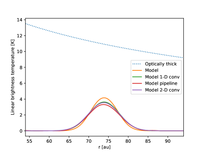
Figure 9: The 1-d radial profiles extracted from the 2-D images in Fig. 10, compared to the original mock ring.

Figure 10: The mock ring test. Left: the input mock ring, inspired by ring 2 of AS 209, assuming a width of $w_{d}=3.07\,\mathrm{au}$. Inclination and position angle are the same as for AS 209. Middle: The mock ring convolved with the Gaussian beam appropriate for AS 209. Right: The mock ring, with noise added, put through the DSHARP imaging pipeline.

References

- Adachi et al. (1976) Adachi, I., Hayashi, C., & Nakazawa, K. 1976, Prog. Theor. Phys., 56, 1756
- ALMA Partnership et al. (2015) ALMA Partnership, Brogan, C. L., Pérez, L. M., et al. 2015, ApJL, 808, L3
- Andrews (2018) Andrews, S. e. a. 2018, ApJ submitted
- Andrews et al. (2009) Andrews, S. M., Wilner, D. J., Hughes, A. M., Qi, C., & Dullemond, C. P. 2009, ApJ, 700, 1502
- Andrews et al. (2016) Andrews, S. M., Wilner, D. J., Zhu, Z., et al. 2016, ApJL, 820, L40
- Auffinger & Laibe (2018) Auffinger, J., & Laibe, G. 2018, MNRAS, 473, 796
- Bai & Stone (2010) Bai, X.-N., & Stone, J. M. 2010, ApJ, 722, 1437
- Barge & Sommeria (1995) Barge, P., & Sommeria, J. 1995, A&A, 295, L1
- Benisty et al. (2017) Benisty, M., Stolker, T., Pohl, A., et al. 2017, A&A, 597, A42
- Béthune et al. (2016) Béthune, W., Lesur, G., & Ferreira, J. 2016, A&A, 589, A87
- Birnstiel et al. (2010) Birnstiel, T., Dullemond, C. P., & Brauer, F. 2010, A&A, 513, A79
- Birnstiel (2018) Birnstiel, T. e. a. 2018, ApJ submitted
- Bitsch et al. (2013) Bitsch, B., Crida, A., Morbidelli, A., Kley, W., & Dobbs-Dixon, I. 2013, Astronomy & Astrophysics, 549, 124
- Brauer et al. (2007) Brauer, F., Dullemond, C. P., Johansen, A., et al. 2007, A&A, 469, 1169
- Casassus et al. (2013) Casassus, S., van der Plas, G., M, S. P., et al. 2013, Nature, 493, 191
- Chiang & Goldreich (1997) Chiang, E. I., & Goldreich, P. 1997, ApJ, 490, 368
- Cieza et al. (2017) Cieza, L. A., Casassus, S., Pérez, S., et al. 2017, ApJL, 851, L23
- Clarke et al. (2018) Clarke, C. J., Tazzari, M., Juhász, A., et al. 2018, The Astrophysical Journal Letters, 866, L6
- D’Alessio et al. (1998) D’Alessio, P., Cantö, J., Calvet, N., & Lizano, S. 1998, ApJ, 500, 411
- Dipierro et al. (2018) Dipierro, G., Ricci, L., Pérez, L., et al. 2018, MNRAS, 475, 5296
- Dong et al. (2016) Dong, R., Zhu, Z., Fung, J., et al. 2016, ApJL, 816, L12
- Drążkowska et al. (2016) Drążkowska, J., Alibert, Y., & Moore, B. 2016, A&A, 594, A105
- Drążkowska & Dullemond (2014) Drążkowska, J., & Dullemond, C. P. 2014, A&A, 572, A78
- Dubrulle et al. (1995) Dubrulle, B., Morfill, G., & Sterzik, M. 1995, Icarus, 114, 237
- Dullemond & Birnstiel (2018) Dullemond, C., & Birnstiel, T. 2018, A&A to be submitted
- Dullemond et al. (2001) Dullemond, C. P., Dominik, C., & Natta, A. 2001, ApJ, 560, 957
- Dullemond & Penzlin (2018) Dullemond, C. P., & Penzlin, A. B. T. 2018, A&A, 609, A50
- Fedele et al. (2017) Fedele, D., Carney, M., Hogerheijde, M. R., et al. 2017, A&A, 600, A72
- Fedele et al. (2018) Fedele, D., Tazzari, M., Booth, R., et al. 2018, A&A, 610, A24
- Flaherty et al. (2018) Flaherty, K. M., Hughes, A. M., Teague, R., et al. 2018, ApJ, 856, 117
- Flock et al. (2013) Flock, M., Fromang, S., González, M., & Commerçon, B. 2013, Astronomy & Astrophysics, 560, 43
- Flock et al. (2015) Flock, M., Ruge, J. P., Dzyurkevich, N., et al. 2015, A&A, 574, A68
- Foreman-Mackey et al. (2013) Foreman-Mackey, D., Hogg, D. W., Lang, D., & Goodman, J. 2013, Publications of the Astronomical Society of the Pacific, 125, 306
- Fromang & Nelson (2009) Fromang, S., & Nelson, R. P. 2009, A&A, 496, 597
- Garaud (2007) Garaud, P. 2007, ApJ, 671, 2091
- Gonzalez et al. (2017) Gonzalez, J.-F., Laibe, G., & Maddison, S. T. 2017, MNRAS, 467, 1984
- Guzmán (2018) Guzmán, V. e. a. 2018, ApJ submitted
- Hartmann et al. (1998) Hartmann, L., Calvet, N., Gullbring, E., & D’Alessio, P. 1998, ApJ, 495, 385
- Huang et al. (2018) Huang, J., Andrews, S. M., Cleeves, L. I., et al. 2018, ApJ, 852, 122
- Huang (2018a) Huang, J. e. a. 2018a, ApJ submitted
- Huang (2018b) —. 2018b, ApJ submitted
- Isella et al. (2016) Isella, A., Guidi, G., Testi, L., et al. 2016, Physical Review Letters, 117, 251101
- Isella (2018) Isella, A. e. a. 2018, ApJ submitted
- Johansen & Klahr (2005) Johansen, A., & Klahr, H. 2005, ApJ, 634, 1353
- Johansen et al. (2007) Johansen, A., Oishi, J. S., Mac Low, M.-M., et al. 2007, Nature, 448, 1022
- Johansen & Youdin (2007) Johansen, A., & Youdin, A. 2007, ApJ, 662, 627
- Kanagawa et al. (2017a) Kanagawa, K. D., Tanaka, H., Muto, T., & Tanigawa, T. 2017a, Publications of the Astronomical Society of Japan, 69, 97
- Kanagawa et al. (2017b) Kanagawa, K. D., Ueda, T., Muto, T., & Okuzumi, S. 2017b, ApJ, 844, 142
- Kataoka et al. (2013) Kataoka, A., Tanaka, H., Okuzumi, S., & Wada, K. 2013, Astronomy & Astrophysics, 557, L4
- Klahr & Henning (1997) Klahr, H. H., & Henning, T. 1997, Icarus, 128, 213
- Kowalik et al. (2013) Kowalik, K., Hanasz, M., Wóltański, D., & Gawryszczak, A. 2013, MNRAS, 434, 1460
- Kratter & Lodato (2016) Kratter, K., & Lodato, G. 2016, ARAA, 54, 271
- Kretke & Lin (2007) Kretke, K. A., & Lin, D. N. C. 2007, ApJL, 664, L55
- Li et al. (2000) Li, H., Finn, J. M., Lovelace, R. V. E., & Colgate, S. A. 2000, ApJ, 533, 1023
- Long et al. (2018) Long, F., Pinilla, P., Herczeg, G. J., et al. 2018, arXiv, arXiv:1810.06044
- Lynden-Bell & Pringle (1974) Lynden-Bell, D., & Pringle, J. E. 1974, MNRAS, 168, 603
- Lyra & Umurhan (2018) Lyra, W., & Umurhan, O. 2018, arXiv, arXiv:1808.08681
- Marino et al. (2015) Marino, S., Perez, S., & Casassus, S. 2015, ApJL, 798, L44
- Okuzumi et al. (2016) Okuzumi, S., Momose, M., Sirono, S.-i., Kobayashi, H., & Tanaka, H. 2016, ApJ, 821, 82
- Okuzumi et al. (2012) Okuzumi, S., Tanaka, H., Kobayashi, H., & Wada, K. 2012, ApJ, 752, 106
- Ono et al. (2016) Ono, T., Muto, T., Takeuchi, T., & Nomura, H. 2016, ApJ, 823, 84
- Perez (2018) Perez, L. e. a. 2018, ApJ submitted
- Pinilla et al. (2012a) Pinilla, P., Benisty, M., & Birnstiel, T. 2012a, A&A, 545, A81
- Pinilla et al. (2012b) Pinilla, P., Birnstiel, T., Ricci, L., et al. 2012b, A&A, 538, A114
- Pinilla et al. (2015) Pinilla, P., Birnstiel, T., & Walsh, C. 2015, A&A, 580, A105
- Pinte et al. (2016) Pinte, C., Dent, W. R. F., Ménard, F., et al. 2016, ApJ, 816, 25
- Powell et al. (2017) Powell, D., Murray-Clay, R., & Schlichting, H. E. 2017, ApJ, 840, 93
- Raettig et al. (2015) Raettig, N., Klahr, H., & Lyra, W. 2015, ApJ, 804, 35
- Ricci et al. (2010) Ricci, L., Testi, L., Natta, A., et al. 2010, A&A, 512, A15
- Rice et al. (2006) Rice, W. K. M., Armitage, P. J., Wood, K., & Lodato, G. 2006, MNRAS, 373, 1619
- Sato et al. (2016) Sato, T., Okuzumi, S., & Ida, S. 2016, Astronomy & Astrophysics, 589, A15
- Schäfer et al. (2017) Schäfer, U., Yang, C.-C., & Johansen, A. 2017, A&A, 597, A69
- Schreiber & Klahr (2018) Schreiber, A., & Klahr, H. 2018, ApJ, 861, 47
- Sheehan & Eisner (2018) Sheehan, P. D., & Eisner, J. A. 2018, ApJ, 857, 18
- Stammler et al. (2017) Stammler, S. M., Birnstiel, T., Panić, O., Dullemond, C. P., & Dominik, C. 2017, A&A, 600, A140
- Takahashi & Inutsuka (2014) Takahashi, S. Z., & Inutsuka, S.-I. 2014, ApJ, 794, 55
- Takahashi & Inutsuka (2016) —. 2016, The Astronomical Journal, 152, 184
- Testi et al. (2003) Testi, L., Natta, A., Shepherd, D. S., & Wilner, D. J. 2003, A&A, 403, 323
- Tsukagoshi et al. (2016) Tsukagoshi, T., Nomura, H., Muto, T., et al. 2016, The Astrophysical Journal Letters, 829, L35
- van der Marel et al. (2013) van der Marel, N., van Dishoeck, E. F., Bruderer, S., et al. 2013, Science, 340, 1199
- van Terwisga et al. (2018) van Terwisga, S. E., van Dishoeck, E. F., Ansdell, M., et al. 2018, A&A, 616, A88
- Weaver et al. (2018) Weaver, E., Isella, A., & Boehler, Y. 2018, ApJ, 853, 113
- Whipple (1972) Whipple, F. L. 1972, in From Plasma to Planet, ed. A. Elvius, 211
- Youdin & Goodman (2005) Youdin, A. N., & Goodman, J. 2005, ApJ, 620, 459
- Youdin & Lithwick (2007) Youdin, A. N., & Lithwick, Y. 2007, Icarus, 192, 588
- Zhang et al. (2015) Zhang, K., Blake, G. A., & Bergin, E. A. 2015, The Astrophysical Journal Letters, 806, L7
- Zhang (2018) Zhang, Z. e. a. 2018, ApJ submitted
- Zhu et al. (2012) Zhu, Z., Nelson, R. P., Dong, R., Espaillat, C., & Hartmann, L. 2012, ApJ, 755, 6