The Disk Substructures at High Angular Resolution Project (DSHARP):
V. Interpreting ALMA maps of protoplanetary disks in terms of a dust model

Abstract

The Disk Substructures at High Angular Resolution Project (DSHARP) is the largest homogeneous high-resolution ($\sim$0$\farcs$035, or $\sim$5\text{\,}\mathrm{a}\mathrm{u}$$) disk continuum imaging survey with ALMA so far. In the coming years, many more disks will be mapped with ALMA at similar resolution. Interpreting the results in terms of the properties and quantities of the emitting dusty material is, however, a very non-trivial task. This is in part due to the uncertainty in the dust opacities, an uncertainty which is not likely to be resolved any time soon. It is also partly due to the fact that, as the DSHARP survey has shown, these disk often contain regions of intermediate to high optical depth, even at millimeter wavelengths and at relatively large radius in the disk. This makes the interpretation challenging, in particular if the grains are large and have a large albedo. On the other hand, the highly structured features seen in the DSHARP survey, of which strong indications were already seen in earlier observations, provide a unique opportunity to study the dust growth and dynamics. To provide continuity within the DSHARP project, its follow-up projects, and projects by other teams interested in these data, we present here the methods and opacity choices used within the DSHARP collaboration to link the measured intensity $I_{\nu}$ to dust surface density $\Sigma_{d}$.

tablenum SIXtablenum

1 Introduction

Dust thermal (sub-)millimeter emission from the outer regions ($r\gtrsim 10\,\mathrm{au}$) of protoplanetary disks has traditionally been considered to be optically thin, because it would require implausible amounts of dust mass to make the disk optically thick at these wavelengths out to many tens of au. Even if it were optically thick, it would produce much higher disk-integrated flux values than are observed (Ricci et al., 2012). If the assumption of low optical depth were true, it would aid the interpretation of sub-millimeter continuum maps in terms of the properties and dynamics of the dust grains, because the observed intensity $I_{\nu}$ would be directly proportional to the underlying dust surface density $\Sigma_{d}$.

Observational results from the past decade have shown that protoplanetary disks do not have simple monotonically decreasing surface density profiles, but consist of multiple narrow rings (e.g., ALMA Partnership et al., 2015; Andrews et al., 2016; Isella et al., 2016; Fedele et al., 2017, 2018; Huang et al., 2018), apparently single massive rings (e.g. Brown et al., 2009; Casassus et al., 2013) but also often non-axisymmetric features such as lopsided rings (e.g. van der Marel et al., 2013), and spirals (e.g. Pérez et al., 2016). These narrow or compact features present concentrations that may be optically thick or moderately optically thick. In between these features, the material is often optically thin.

This is both a curse and a blessing. Such optical depth effects make the interpretation of the data more difficult. In particular the spectral slope variations at (sub-)millimeter wavelengths ($I_{\nu}\propto\nu^{\alpha_{\mathrm{mm}}}$) across rings and gaps are strongly affected, perhaps even dominated, by these effects. But optical depth effects also provide new opportunities to measure the properties of the dust. An example of this is the scattering of its own thermal emission, and the induced polarized millimeter emission (Kataoka et al., 2015). Another example is when dust rings extinct part of the CO line emission from the back side of a disk (Isella et al. 2018).

But there is, of course, the major uncertainty in the dust opacity law. This is a long-standing problem (Beckwith & Sargent, 1991) that still has not been resolved. This is in part because dust in protoplanetary disks, in particular the large grains seen as settled grains in a thin mid-plane layer, is very different from the dust in the interstellar medium. In part it is, however, also due to uncertainties in the numerical and conceptual challenges in computing opacities. When comparing computed opacities with laboratory measured opacities in the millimeter range, one often sees discrepancies of up to a factor of 10 or more (e.g. Demyk et al., 2017).

By inspecting the (sub-)millimeter spectral slope $\alpha_{\mathrm{mm}}$ we can learn something about the grain size distribution and the opacity law (e.g. Beckwith & Sargent, 1991; Testi et al., 2003; Wilner et al., 2005). With high angular resolution observations this can now be done as a function of radial coordinate in the disk (e.g., Guilloteau et al., 2011; Isella et al., 2010; Pérez et al., 2012), and shows that bright rings have shallower slopes than the dark annuli between them (e.g. ALMA Partnership et al., 2015; Tsukagoshi et al., 2016; Huang et al., 2018). However, changes in the spectral slope can also be caused by optical depth effects. The results of the ALMA Large Program DSHARP (Andrews et al. 2018) show that these dust rings often have an optical depth close to unity (Huang et al. 2018a, Dullemond et al. 2018, Isella et al. 2018).

With the detailed spatial information of the substructures in millimeter continuum and line maps of protoplanetary disks that ALMA is providing, it becomes increasingly important to discuss the details of the opacities used and the methods applied to translate the observations into information about the underlying dust grains.

The present paper is meant to give an overview of the methods used and choices made by the DSHARP collaboration to make this translation. We do not claim in any way that our choices and methods are better than those used by others, nor that we can resolve any of the uncertainties of the opacities. Instead, this paper describes our methods and choices, and we provide an easy-to-use python module and a set of example calculations for the reproduction of these opacities and variants of them, as well as for handling some of the optical depth effects discussed in this paper.

The structure of this paper is as follows: In Section 2 we discuss our choices for computing the dust opacities, and present our Python tools that are publicly available. In Section 3 we apply these opacities to simple size distribution models, starting with a standard power-law model, and ending in Section 4 with the analytic steady-state dust coagulation/fragmentation size distribution of Birnstiel et al. (2011, henceforth B11), again including the corresponding Python scripts. Finally, in Section 5 we present a very simple model to link the observed thermal emission to the observed extinction of back-side CO line emission (Isella et al. 2018).

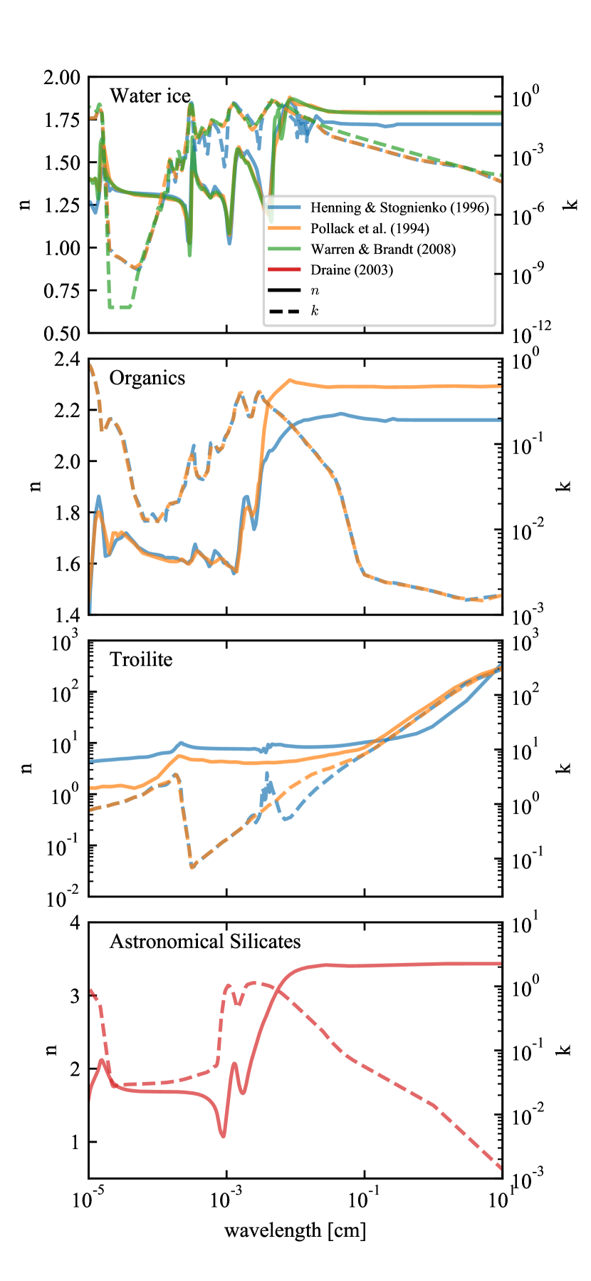
Figure 1: Optical constants used in this work (see Table 1), compared to other literature data. Solid lines denote $n$ on the left axis and dashed lines denote $k$ on the right axis.

2 DSHARP Dust Opacities

As discussed above, the goal of this paper is not to provide a “better” dust opacity model, but instead a transparent model based on open-source software that is easy to reproduce or to modify. To this end, we follow seminal works regarding protoplanetary disk composition and grain structure (Pollack et al., 1994, henceforth P94) that are widely used throughout the literature and we use updated optical constants where available. To stay comparable to previously used opacities (and thus the resulting mass or surface density estimates), we chose to assume particles without porosity. This is a pragmatic choice instead of a realistic one for protoplanetary disks since since at least the initial growth phase involves larger porosities (Kempf et al., 1999; Ormel et al., 2007; Zsom et al., 2010; Okuzumi et al., 2012; Krijt et al., 2015).

P94 and subsequent work by D’Alessio et al. (2001) chose a mixture of water ice, astronomical silicates, troilite, and refractory organic material. The water fraction that was used in those works (around 60% by volume) was, however in disagreement with typically observed disk spectral energy distributions (SEDs), as pointed out by D’Alessio et al. (2006) and Espaillat et al. (2010) who reduced the water fraction to 10% of the value used in P94. Since comets are thought to be a relatively pristine sample of the planet forming material, we chose a water fraction of 20% by mass, in agreement with measurements of comet 67P/Churyumov-Gerasimenko (Pätzold et al., 2016).

To calculate mass absorption or scattering coefficients $\kappa_{\nu}^{\mathrm{abs}}$ or $\kappa_{\nu}^{\mathrm{sca}}$, we assume vacuum as embedding medium and furthermore need the complex refractive indices $m(\lambda)=n(\lambda)+\mathrm{i}\,k(\lambda)$ which are functions of wavelength $\lambda$. These refractive index data will be called optical constants for simplicity.

The optical constants of water used in D’Alessio et al. (2001) were from Warren (1984) who gives tables for various temperatures. Henning & Stognienko (1996) used optical constants from Hudgins et al. (1993) (amorphous ice at at 100 K) between 2.5 and $200\text{\,}\mu\mathrm{m}$ and the constants from P94 for the remaining wavelengths ranges. In this work, we use the more recent data from Warren & Brandt (2008). However the differences to previous works are small (see Figure 1).

The astronomical silicates used in D’Alessio et al. (2001) took a constant $k$ value for $\lambda>$800\text{\,}\mu\mathrm{m}$$. Henning & Stognienko (1996) argued (their section 5.1) that $k\propto\lambda^{-1}$ is usually assumed, but that Campbell & Ulrichs (1969) indeed measured a high value of $k=0.05$ at $2.7\text{\,}\mathrm{m}\mathrm{m}$ (see Figure 1). Nevertheless, we use the opacities from Draine (2003) for astronomical silicates without increasing $k$.

For troilite and refractory organics, we use the optical constants from Henning & Stognienko (1996). For troilite, the constants are partly based on Begemann et al. (1994) (in the range of 10 to $500\text{\,}\mu\mathrm{m}$), with longer and shorter ranges taken from P94. Henning & Stognienko (1996) also performed Kramers-Kronig analysis on the organics optical constants of P94 which yielded little differences. The Henning & Stognienko (1996) data sets for troilite and refractory organics are available online, and are included in our opacity module with kind permission from Thomas Henning. The optical constants used in this work are shown in Figure 1.

Deriving optical constants for a mix of materials is a challenging task as it depends on the detailed structure of the composite particle. No general solution can be given. For more complex setups, computationally expensive numerical models need to be used. For some limiting cases analytical expressions can be given. These are typically called the Maxwell-Garnett rule (valid for inclusions in a background “matrix”) and the Bruggemann rule, for a homogeneous mix without a dominant matrix. Details can be found in Bohren & Huffman (1998) whose notation we will follow.

If $f_{i}$ denotes the volume fractions of the $N$ inclusions ($i=1\ldots N$) and $\epsilon_{i}=m_{i}^{2}$ the dielectric functions of the inclusions (with refractive indices $m_{i}$), while $f_{m}$ and $\epsilon_{m}$ are the corresponding values for the matrix, then the Maxwell-Garnett rule for spherical inclusions yields the mixed dielectric function

$$\bar{\epsilon} =\frac{(1-f)\,\epsilon_{m}+\sum_{i=1}^{N}{f_{i}\,\beta_{i}\,\epsilon_{i}}}{1-f+\sum_{i=1}^{N}{f_{i}\,\beta_{i}}},$$ (1)

where

$$\beta_{i} =\frac{3\,\epsilon_{m}}{\epsilon_{i}+2\,\epsilon_{m}},$$ (2)

$$f =\sum_{i=1}^{N}{f_{i}}.$$ (3)

For the case of the Bruggeman rule, the mixed material itself acts as matrix and the mixed dielectric function can be calculated by solving for $\bar{\epsilon}$ in the relation

$$\sum_{i=1}^{N}{f_{i}\,\frac{\epsilon_{i}-\bar{\epsilon}}{\epsilon_{i}+2\,\bar{\epsilon}}}=0.$$ (4)

Both the Bruggeman and the Maxwell-Garnett rule are implemented in our opacity module. However for the compact mixture of materials specified above and in Table 1, the Bruggeman rule is the appropriate choice. For this dust model, the resulting effective medium optical constants are shown in Figure 2.

Our opacity module includes a subroutine to do Mie opacity calculations using a Fortran90 subroutine for performance. This Fortran90 code is based on a Fortran70 version by Bruce Draine which itself is derived from the original Mie code published by Bohren & Huffman (1998). To avoid strong and artificial Mie interferences, we do not use single-grain-size opacities, but instead calculate the opacity for 40 linearly spaced bins within each grain size bin and average over those opacity values to calculate an averaged opacity value for every size bin (each bin is $0.035\text{\,}\mathrm{d}\mathrm{e}\mathrm{x}$ in size). The resulting absorption and scattering opacities are shown in Figure 3 and are available from the module repository.

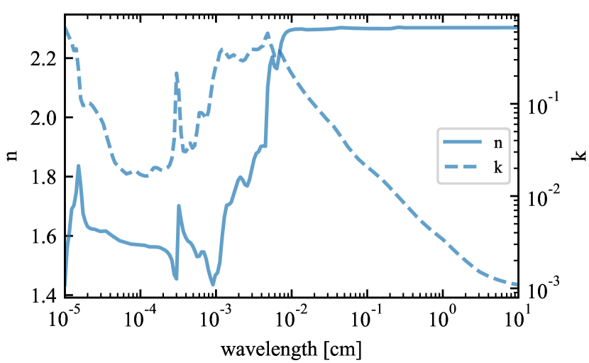
Figure 2: Effective medium optical constants that are used within the DSHARP collaboration, derived with the Bruggeman rule (Eq. 4).

Figure 3: Absorption (top) and scattering (bottom) opacity as function of wavelength $\lambda$ and particle size $a$, based on Mie calculations using the optical constants from Figure 2.

Table 1: Dust composition used in the DSHARP collaboration

Material	References	bulk density	mass fraction	vol. fraction
		[g/cm3]
Water ice	Warren & Brandt (2008)	0.92	0.2000	0.3642
Astronomical Silicates	Draine (2003)	3.30	0.3291	0.1670
Troilite	Henning & Stognienko (1996)	4.83	0.0743	0.0258
Refractory organics	Henning & Stognienko (1996)	1.50	0.3966	0.4430

Note. — The bulk density of the mix is $\rho_{\mathrm{s}}=$1.675\text{\,}\mathrm{g}\,\mathrm{c}\mathrm{m}^{-3}$$.

3 Grain-size averaged opacities

It is known that dust grains in protoplanetary disks are not “mono-disperse”, i.e., at a given radius in the disk the dust does not consist of only a single size, or a narrow size distribution. Perhaps the most spectacular evidence of this is found in the source IM Lup. When observed at near-infrared wavelengths, this disk shows a strongly flaring geometry (Avenhaus et al., 2018). Clearly, a substantial amount of fine-grained dust is suspended several scale heights above the mid-plane, and is continuously replenished by turbulent stirring. When observed at millimeter wavelengths, however, we see a disk with small-scale ring and spiral substructure that can only be explained if the geometry of this dust layer is vertically geometrically thin (e.g., Pinte et al., 2008, Huang et al. 2018b). This must be of a grain population that is vastly larger (and/or more compact) than the grains seen in the near-infrared. Posed more precisely: IM Lup features at least two dust grain populations, one with very small Stokes number, and therefore vertically extended, and one with much larger Stokes number, and therefore vertically flat due to settling.

It is reasonable to expect that the dust population in fact consists of a continuous size distribution instead of just two distinct sizes. This is what is expected from models of dust coagulation which include fragmentation (Weidenschilling, 1984; Dullemond & Dominik, 2005; Brauer et al., 2008; Birnstiel et al., 2010). These populations change with time, as the grains drift and grow at different rates. The complexity of this process makes it hard to define a simple “one-size-fits-all” dust opacity model to be used for interpreting millimeter continuum maps of protoplanetary disks. On the other hand, detailed coagulation/fragmentation modeling is numerically expensive, and it is not feasible to analyze all data with such full-fledged models.

Many authors use therefore a compromise by assuming that the dust grain size distribution follows a simple power-law with a cut-off at small and large grain sizes,

$$n(a)\propto\,\begin{cases}a^{-q}&\text{for}\,a_{\mathrm{min}}\leq a\leq a_{\mathrm{max}}\\ 0&\text{else},\end{cases}$$ (5)

where the total dust density is defined as $\rho_{\mathrm{d}}=\int_{0}^{\infty}\,n(a)\,m(a)\,\mathrm{d}a$ with $m(a)$ being the mass of a dust particle of radius $a$. The resulting opacity at (sub-)millimeter wavelengths is found to be less sensitive to the minimum grain radius $a_{\mathrm{min}}$, but much more so to the maximum particle size $a_{\mathrm{max}}$ as well as the power-law index $q$ (Ricci et al., 2010; Draine, 2006).

Table 2: Dust size distributions used throughout this paper.

Acronym	Description	References
MRN	power-law, $q=3.5$ or	Mathis et al. (1977),
	$q=2.5$	D’Alessio et al. (2001),
		Eq. 5
B11	analytic fits to detailed simulations of growth and fragmentation	Birnstiel et al. (2011)
B11S	simplified versions of B11	Appendix A

The index $q$ was found to be around $3.5$ for interstellar extinction measurements (e.g., Mathis et al., 1977, henceforth MRN) which is consistent with collisional cascades (Dohnanyi, 1969; Tanaka et al., 1996) and also found to be consistent with sub-millimeter observations of debris disks (Ricci et al., 2015). However, the physics of debris disks is very different from gaseous protoplanetary disks. One way out is to use simplified dust coagulation/fragmentation models. For instance, B11 presented an analytic multi-power-law fit to the results of the full-fledged numerical dust coagulation/fragmentation models. A summary of the size distributions and the acronyms used throughout this paper can be found in Table 2.

In the following, we will use the DSHARP opacity model of Section 2 and apply it to a simple power-law size distribution. We compare those results to the ones obtained if the analytic coagulation model fits of B11 are used. The Python script for creating the resulting size-averaged opacities is publicly available in the module repository.

The total absorption opacity $\kappa_{\nu}^{\mathrm{abs,tot}}$ of a particle size distribution $n(a)$ at frequency $\nu$ is calculated from the size-dependent opacity $\kappa_{\nu}^{\mathrm{abs}}(a)$ via

$$\kappa_{\nu}^{\mathrm{abs,tot}}=\frac{\int_{a_{\mathrm{min}}}^{a_{\mathrm{max}}}n(a)\,m(a)\,\kappa_{\nu}^{\mathrm{abs}}(a)\,\mathrm{d}a}{\int_{a_{\mathrm{min}}}^{a_{\mathrm{max}}}n(a)\,m(a)\,\mathrm{d}a}.$$ (6)

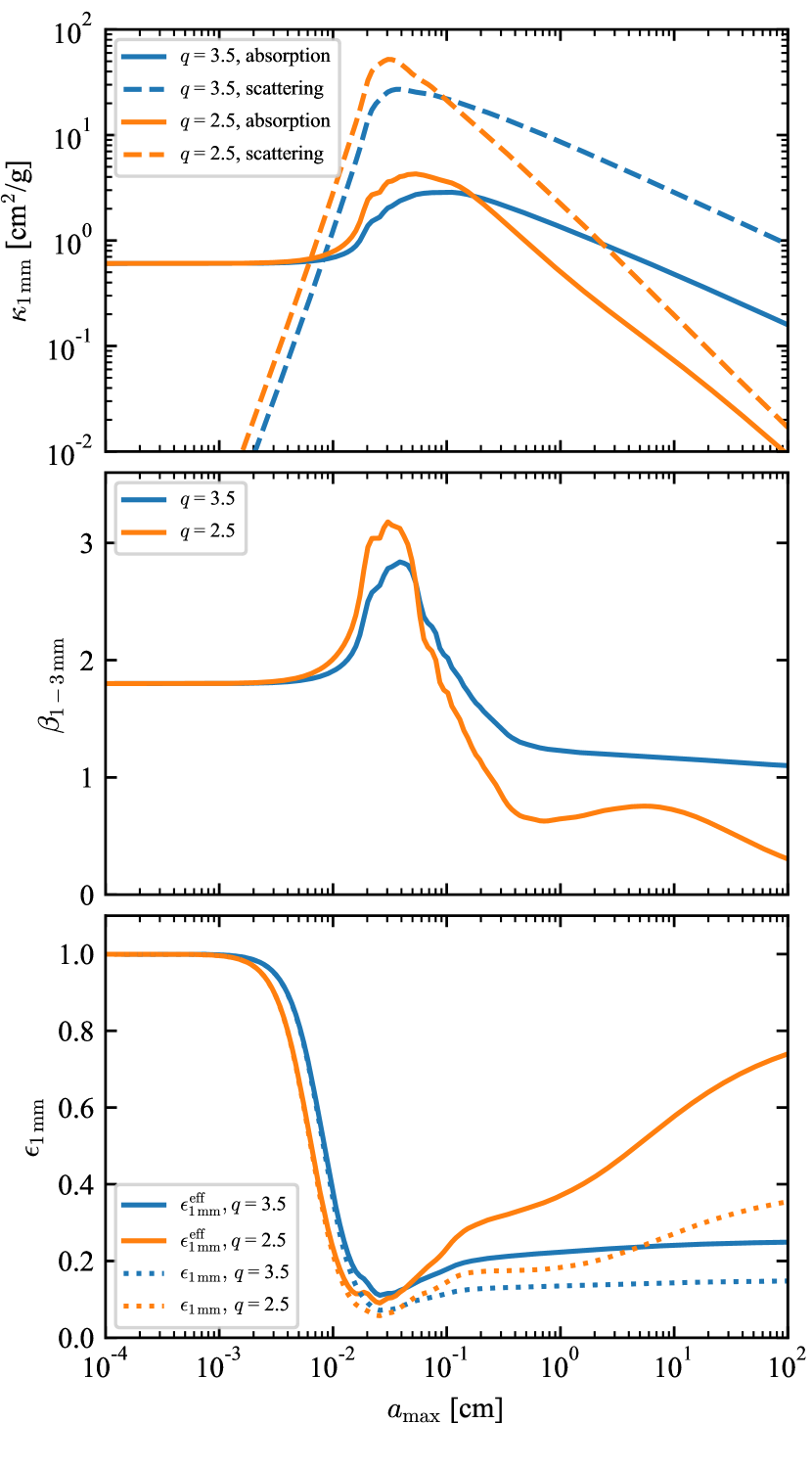
Figure 4: Particle size averaged opacities. Top: scattering ($\kappa_{\nu}^{\mathrm{sca,tot}}$) and absorption ($\kappa_{\nu}^{\mathrm{abs,tot}}$) opacity at $1\text{\,}\mathrm{m}\mathrm{m}$. Middle: spectral index $\beta$ measured at 1-$3\text{\,}\mathrm{m}\mathrm{m}$. Bottom: extinction probability $\epsilon^{\mathrm{eff}}_{$1\text{\,}\mathrm{m}\mathrm{m}$}$ (see Section 5). The assumed size distribution for these averaged properties follows a power-law $n(a)\propto a^{-q}$ from the minimum size of ${10}^{-5}\text{\,}\mathrm{c}\mathrm{m}$ up to maximum size $a_{\mathrm{max}}$. Blue lines denote the MRN-slope of $q=3.5$, orange lines correspond to $q=2.5$.

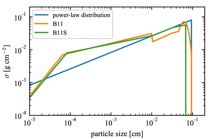
Figure 5: Particle size distributions used in Section 3. $\sigma(a)$ is the surface density per logarithm in particle size, see Eq. A10. The blue line is a truncated power-law with $q=3.5$. The orange line is a size distribution fit in coagulation/fragmentation equilibrium from B11, where parameters were chosen to result in a maximum particle size of $1\text{\,}\mathrm{m}\mathrm{m}$. The green line labeled B11S is a simplified version of the B11 fit using only a broken power-law. This neglects finer details of the fit, but avoids calculating collision velocities.

The top panel in Figure 4 shows the total absorption and scattering opacities at a wavelength of $1\text{\,}\mathrm{m}\mathrm{m}$ for a particle size distribution with $a_{\mathrm{min}}=${10}^{-5}\text{\,}\mathrm{c}\mathrm{m}$$ as function of $a_{\mathrm{max}}$. The bottom panel shows the spectral index $\beta=\partial\ln\kappa_{\nu}^{\mathrm{abs,tot}}/\partial\ln\nu$. Similar trends as in Ricci et al. (2010) are observed: changes in the size distribution index $q$ mainly affect the asymptotic behavior at long wavelengths and the strength of the Mie interference at $a_{\mathrm{max}}\sim\frac{\lambda}{2\pi}$. Figure 4 also shows that for size distributions that extend up to $a_{\mathrm{max}}\gtrsim$100\text{\,}\mu\mathrm{m}$$, the scattering opacity $\kappa_{\nu}^{\mathrm{sca,tot}}$ exceeds the absorption opacity $\kappa_{\nu}^{\mathrm{abs,tot}}$.

Three different particle size distributions were chosen, that have the same maximum particle size $a_{\mathrm{max}}$ of $1\text{\,}\mathrm{m}\mathrm{m}$, however one follows the MRN-like size-exponent of $q=3.5$, while the other two distribution are steady-state size distributions where continuous particle growth and fragmentation lead to a stationary size distribution. The first of these (orange line in Figure 5) is from detailed analytical fits to numerical simulations from B11. The second steady-state distribution, shown in green in Figure 5, is a simplified version of these fits. This implements only the piecewise power-laws from B11 and ignores finer details. This avoids calculating collision velocities for all particle sizes and thus makes the calculation easier and faster (see Appendix A). This simplified fit still captures the important aspects of the simulated distributions much better than the two-power-law fits used in Birnstiel et al. (2015) and Ormel & Okuzumi (2013). Especially for large particle sizes, the two-power-law fits can underpredict the number of small particles available.

Wavelength-dependent opacities for all three distributions have been calculated and are shown in Figure 6 in comparison with opacities used in the literature. It can be seen that the overall behavior is – by construction – similar to the opacities in D’Alessio et al. (2001) or Andrews et al. (2009) with slightly different behavior at long wavelengths. Differences in the $\mu$m wavelength range are mainly due to the different amounts of small grains present in the distributions due to the knee in the steady state distributions. This comes from the fact that smaller particles that move at higher Brownian motion velocities are more efficiently incorporated into larger particles. It can be seen that the two different fitting methods (labeled B11 and B11S) yield virtually identical opacities. The small differences to the simple MRN-power-law stems from the fact that parameters were chosen to yield the same $a_{\mathrm{max}}$. As seen from Figure 4, $a_{\mathrm{max}}$ is the most important parameter influencing the size-averaged opacity.

4 Mean Opacities of steady-state size distributions

The simplified fits labeled B11S are compared to the more detailed fits from B11 in Figure 7. Given the uncertainty in the details of collision models (see, Güttler et al., 2010; Windmark et al., 2012, for example), and for ease of reproduction, we will be using the B11S fits in the following. They are explained in Appendix A. Throughout this paper, we assume a dust-to-gas mass ratio of 0.01 and consider size distributions integrated over height; settling will cause the size distribution to depend on the vertical position above the mid-plane.

Figure 7 shows how the particle size distribution in steady-state varies with the gas temperature $T$, the gas surface density $\Sigma_{\mathrm{g}}$, the fragmentation threshold velocity $v_{\mathrm{frag}}$, and the turbulence parameter $\alpha$ (Shakura & Sunyaev, 1973). It can be seen, that the position in the knee of the distribution at size $a_{\mathrm{BT}}$ (cf. Equation 37 in B11) has only a weak dependence on those parameters, however that the maximum particle size $a_{\mathrm{max}}$ is a strong function of these parameters (quadratic in $v_{\mathrm{f}}$, linear in all others). As such, it also affects the Planck and Rosseland mean opacities,

$$\bar{\kappa}_{\mathrm{P}}(T) =\frac{\int_{0}^{\infty}\kappa_{\nu}^{\mathrm{abs,tot}}\,B_{\nu}(T)\,\mathrm{d}\nu}{\int_{0}^{\infty}B_{\nu}(T)\,\mathrm{d}\nu},$$ (7)

$$\bar{\kappa}_{\mathrm{R}}(T) =\left(\frac{\int_{0}^{\infty}\frac{1}{\kappa_{\nu}^{\mathrm{ext,tot}}}\,\frac{\mathrm{d}B_{\nu}(T)}{\mathrm{d}T}\,\mathrm{d}\nu}{\int_{0}^{\infty}\frac{\mathrm{d}B_{\nu}(T)}{\mathrm{d}T}\,\mathrm{d}\nu}\right)^{-1},$$ (8)

since now not only the Planck spectrum $B_{\mathrm{\nu}}(T)$ is temperature dependent, but also the size-averaged opacities $\kappa_{\nu}^{\mathrm{abs,tot}}$, and $\kappa_{\nu}^{\mathrm{ext,tot}}$. This means that the mean opacities are additionally dependent on other physical parameters, $\Sigma_{\mathrm{g}},v_{\mathrm{frag}}$, and $\alpha$.

As an example, Figure 8 shows the Rosseland and Planck mean opacities for two cases: a MRN-size distribution (as in Figure 5) and the steady-state distributions B11 and B11S as a function of temperature. It can also be seen, that differences between the two steady-state distributions are small, allowing the simpler model to be used without caveats. It can be seen that for the fiducial values of $M_{\star}=M_{\odot}$, $r=$1\text{\,}\mathrm{a}\mathrm{u}$$, $v_{\mathrm{frag}}=$100\text{\,}\mathrm{c}\mathrm{m}\mathrm{/}\mathrm{s}$$, and $\alpha=${10}^{-3}\text{\,}$$, high-temperature mean opacities are generally higher for steady-state distributions owing to the fact that the knee at $\mu$m sizes produces more small grains for the same $a_{\mathrm{max}}$ than a single power-law size distribution. Furthermore high temperatures tend to produce smaller $a_{\mathrm{max}}$ than $1\text{\,}\mathrm{m}\mathrm{m}$ which additionally increases the amount of small particles that contribute most to the mean opacities. The shaded areas in Figure 8 are covering the ranges $$1\text{\,}\mathrm{K}$\leq T\leq$1500\text{\,}\mathrm{K}$$, $$50\text{\,}\mathrm{c}\mathrm{m}\,\mathrm{s}^{-1}$\leq v_{\mathrm{frag}}\leq$3\text{\times}{10}^{3}\text{\,}\mathrm{c}\mathrm{m}\,\mathrm{s}^{-1}$$, $${10}^{-5}\text{\,}$\leq\alpha\leq${10}^{-1}\text{\,}$$, $$1\text{\,}\mathrm{g}\,\mathrm{c}\mathrm{m}^{-2}$\leq\Sigma_{\mathrm{g}}\leq${10}^{4}\text{\,}\mathrm{g}\,\mathrm{c}\mathrm{m}^{-2}$$. It should be noted that the distributions discussed here only apply to those parts of the disk where particles reach the fragmentation barrier $a_{\mathrm{frag}}$ – this is only possible if 1) collision velocities are high enough (i.e. the root in Eq. A8 is real), and 2) fragmentation is more important in limiting particle growth than drift, which is the case if (see Birnstiel et al., 2015)

$$\alpha>\frac{\left|\gamma\right|\,\Sigma_{\mathrm{g}}}{3\,\Sigma_{\mathrm{d}}}\left(\frac{v_{\mathrm{frag}}}{V_{\mathrm{K}}}\right),$$ (9)

where $\gamma$ is the radial logarithmic pressure gradient $\partial\ln P/\partial\ln r$ and $V_{\mathrm{K}}$ the Keplerian orbital velocity. If the drift limit applies, the size distribution will contain more mass at the largest sizes and is more strongly dependent on global redistribution of particles. These non-local processes can be approximated as in Birnstiel et al. (2015), however the accuracy of these approximations are likely only good enough for applying them to the long-wavelength opacity. Short wavelengths are too sensitive to small changes in the amount of small grains, which in turn depend sensitively on radial mixing, and details of the collisional model.

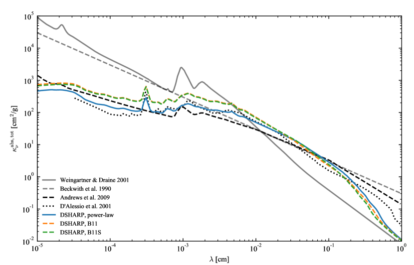
Figure 6: Wavelength dependency of size averaged absorption opacities using a power-law size distribution ($a_{\mathrm{min}}=${10}^{-5}\text{\,}\mathrm{c}\mathrm{m}$$, $a_{\mathrm{max}}=$1\text{\,}\mathrm{m}\mathrm{m}$$, $q=3.5$) and opacity values used in the literature for comparison.

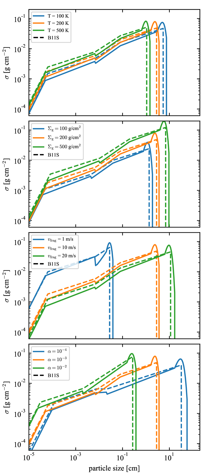
Figure 7: Comparison of fitting functions of B11 and the simplified fitting function (see Appendix A). The fiducial model is denoted by the orange line and its parameters are given in Section 4.

5 Dust emission and extinction from a thin dust layer with scattering

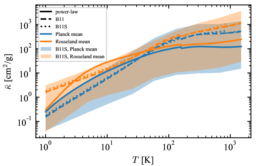
Figure 8: Planck (blue) and Rosseland (orange) mean opacities for steady state size distributions (dashed and dotted lines) and for a power-law distribution with fixed $a_{\mathrm{max}}=$1\text{\,}\mathrm{m}\mathrm{m}$$ (solid lines). The fits (dashed and dotted lines) used fixed parameters as in Figure 5, only varying the temperature. The shaded regions show the range of opacities if the other parameters affecting the fits are varied within reasonable ranges (see Section 4). For temperatures above the water sublimation temperature, the water ice was removed from the material mix.

For protoplanetary disks, it is mostly assumed that only the absorption opacity $\kappa_{\nu}^{\mathrm{abs}}$, not the scattering opacity, matters. For optically thin dust layers this is indeed appropriate. Recently, the importance of scattering and its effects on (sub-)millimeter polarization of disks was pointed out by Kataoka et al. (2015). In the DSHARP campaign we have seen that the optical depths are not that low ($0.1\lesssim\tau\lesssim 0.6$, see Dullemond et al. 2018). Furthermore, the CO line extinction data of HD 163296 discussed by Isella et al. (2018) suggest that the dust layer has an extinction optical depth close to unity (see also Guzman et al. 2018). Even if the absorption optical depth is substantially below 1, the total extinction (absorption + scattering) can easily exceed unity, if the grains are of similar size to the wavelength. For $a\simeq\lambda/2\pi=$0.13\text{\,}\mathrm{c}\mathrm{m}$/2\pi=$0.02\text{\,}\mathrm{c}\mathrm{m}$$ the albedo of the grain can, in fact, be as high as 0.9 (see Figure 4 and Appendix B).

The inclusion of scattering complicates the radiative transfer equation enormously. Strictly speaking a full radiative transfer calculation, for instance with a Monte Carlo code, is necessary. However, in the spirit of this paper we wish to find a simple approximation to handle this without resorting to complex numerical simulation.

There are two issues to be solved: One is: what thermal emission will a non-optically-thin dust layer produce if scattering is taken into account? The other is: how do we compute the extinction coefficient to be used in the CO line extinction analysis?

For the first issue, we will outline here a simple two-stream radiative transfer approach to the problem. We will assume that the dust seen in the ALMA observations is located in a geometrically thin layer at the mid-plane, so we can use the 1-D slab geometry approach. We will assume that the scattering is isotropic. This may be a bad approximation, especially for $2\pi a\gg\lambda$. To reduce the impact of this approximation we replace the scattering opacity $\kappa_{\nu}^{\mathrm{sca}}$ with

$$\kappa_{\nu}^{\mathrm{sca,eff}}=(1-g_{\nu})\,\kappa_{\nu}^{\mathrm{sca}}$$ (10)

where $g_{\nu}$ is the usual forward-scattering parameter (the expectation value of $\cos\theta$, where $\theta$ is the scattering angle). According to Ishimaru (1978), this approximation works well in optically thick media.

We will now follow the two-stream / moment method approach from Rybicki & Lightman (1991) to derive the solution to the emission/absorption/scattering problem in this slab. The slab is put between $z=-\tfrac{1}{2}\Delta z$ and $z=+\tfrac{1}{2}\Delta z$ and we assume a constant density of dust between these two boundaries. The mean intensity $J_{\nu}(z)$ of the radiation field then obeys the equation

$$\frac{1}{3}\frac{d^{2}J_{\nu}}{d\tau_{\nu}^{2}}=\epsilon_{\nu}\big{(}J_{\nu}-B_{\nu}(T_{d})\big{)}$$ (11)

where

$$\tau_{\nu}=\rho_{d}\,(\kappa_{\nu}^{\mathrm{abs}}+\kappa_{\nu}^{\mathrm{sca,eff}})z\equiv\rho_{d}\,\kappa_{\nu}^{\mathrm{tot}}z$$ (12)

with $\rho_{d}$ being the dust density, and

$$\epsilon^{\mathrm{eff}}_{\nu}=\frac{\kappa_{\nu}^{\mathrm{abs}}}{\kappa_{\nu}^{\mathrm{abs}}+\kappa_{\nu}^{\mathrm{sca,eff}}}$$ (13)

The boundary conditions at $z=\pm\tfrac{1}{2}\Delta z$ are

$$\frac{dJ_{\nu}}{d\tau_{\nu}}=\mp\sqrt{3}J_{\nu}$$ (14)

This leads to the following solution:

$$\frac{J_{\nu}(\tau_{\nu})}{B_{\nu}(T_{d})}=1-b\,\left(e^{-\sqrt{3\epsilon^{\mathrm{eff}}_{\nu}}\left(\tfrac{1}{2}\Delta\tau-\tau_{\nu}\right)}+e^{-\sqrt{3\epsilon^{\mathrm{eff}}_{\nu}}\left(\tfrac{1}{2}\Delta\tau+\tau_{\nu}\right)}\right)$$ (15)

where $\Delta\tau=\rho_{d}\,\kappa_{\nu}^{\mathrm{tot}}\Delta z$, and $b$ is

$$b=\left[(1-\sqrt{\epsilon^{\mathrm{eff}}_{\nu}})e^{-\sqrt{3\epsilon^{\mathrm{eff}}_{\nu}}\Delta\tau}+1+\sqrt{\epsilon^{\mathrm{eff}}_{\nu}}\right]^{-1}$$ (16)

Given this solution for the mean intensity $J_{\nu}(\tau_{\nu})$ we can now numerically integrate the formal transfer equation along a single line of sight passing through the slab at an angle $\theta$:

$$\mu\frac{dI_{\nu}(\tau_{\nu})}{d\tau_{\nu}}=\epsilon^{\mathrm{eff}}_{\nu}B_{\nu}(T_{d})+(1-\epsilon^{\mathrm{eff}}_{\nu})J_{\nu}(\tau_{\nu})-I_{\nu}(\tau_{\nu})$$ (17)

where $\mu=\cos\theta$. We start at $\tau_{\nu}=-\tfrac{1}{2}\Delta\tau$ with $I_{\nu}=0$, and integrate to $\tau_{\nu}=+\tfrac{1}{2}\Delta\tau$. The resulting $I_{\nu}^{\mathrm{out}}=I_{\nu}(\tfrac{1}{2}\Delta\tau)$ is the intensity that is observed by the telescope. An approximation for $I_{\nu}^{\mathrm{out}}$ which works well to within a few percent is the following modified version of the Eddington-Barbier approximation:

$$I_{\nu}^{\mathrm{out}}\simeq\left(1-e^{-\Delta\tau/\mu}\right)\,S_{\nu}\left((\tfrac{1}{2}\Delta\tau-\tau_{\nu})/\mu=2/3\right)$$ (18)

where

$$S_{\nu}(\tau_{\nu})=\epsilon^{\mathrm{eff}}_{\nu}B_{\nu}(T_{d})+(1-\epsilon^{\mathrm{eff}}_{\nu})J_{\nu}(\tau_{\nu})$$ (19)

is the source function. In the optically thin case, when $\Delta\tau/\mu<2/3$, the value of $S_{\nu}$ is taken at the edge of the slab. The results are shown in Figure 9.

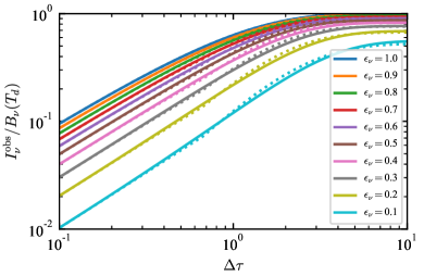
Figure 9: The intensity $I_{\nu}$, in units of the Planck function, emerging from a slab seen face on, with total optical depth $\Delta\tau$, a constant temperature, and an albedo of $\eta_{\nu}=1-\epsilon^{\mathrm{eff}}_{\nu}$. See Section 5 for details. The solid lines are the results of numerical integration of Eq. 17. The dotted lines are the result of the modified Eddington-Barbier approximation (Eq. 18).

For small optical depth ($\Delta\tau\ll 1$) the role of scattering vanishes, and the solution approaches: $I_{\nu}^{\mathrm{out}}\rightarrow\epsilon^{\mathrm{eff}}_{\nu}\Delta\tau B_{\nu}(T_{d})/\mu$. This is the same limiting solution as when $\kappa_{\nu}^{\mathrm{sca}}$ is set to zero but $\kappa_{\nu}^{\mathrm{abs}}$ is kept the same. For high optical depth the outcoming intensity does not saturate to the Planck function, but a bit below, if the albedo is non-zero. This is the well-known effect that scattering makes objects appear cooler than they really are.

Now let us turn to the second issue to be considered: how to calculate the actual extinction coefficient for the CO line extinction analysis. At first sight the answer is simple:

$$\kappa_{\nu}^{\mathrm{ext}}=\kappa_{\nu}^{\mathrm{abs}}+\kappa_{\nu}^{\mathrm{sca}}$$ (20)

where we use $\kappa_{\nu}^{\mathrm{sca}}$, not $\kappa_{\nu}^{\mathrm{sca,eff}}$, for the scattering. This is, in fact, the correct answer for the case in which the emitting CO line emitting layer is far behind the extincting dust layer, where “far” is defined in comparison to the width of the extincting dust ring. If this condition is, however, not met, then the scattering will not reduce the CO line intensity as much as naively expected. CO line photons that are heading elsewhere might then, in fact, get scattered into the line of sight. This effect is exacerbated for the case of small-angle scattering. One can therefore argue that this effect reduces the extinction of the CO line emission by the dust layer. For the case of HD 163296 (Isella et al. 2018) it appears that these effects are not too strong, so a first analysis without accounting for this is in order. A final answer may, however, require a full treatment of 3-D radiative transfer.

6 Summary

In this paper we present methods for translating observed dust emission and extinction used in the DSHARP campaign, which can also be used by other work. The DSHARP opacities presented here are merely a choice, based on reasonable assumptions. They provide the standard used within the DSHARP campaign.

We further explore how steady-state size distributions in a coagulation-fragmentation equilibrium affect dust opacities by introducing dependencies on temperature, surface density, turbulence and material properties. We provide simplified fits to analytical functions and show the range of Rosseland and Planck mean opacities covered for a wide range of parameter choices.

Given the large albedo at (sub-)millimeter wavelength ranges, we derive solutions to the radiative transfer equation for a homogeneous medium with scattering and absorption. Together with the DSHARP dust model, and based on the measurements of Isella et al. (2018), we find that the particles in the rings of HD163296 should be at least $0.2\text{\,}\mathrm{c}\mathrm{m}$ of size.

Along with this paper, we present publicly available Python scripts that contain the optical data of many literature materials. In addition to that, functions are available for mixing optical constants with effective medium theory, for calculating opacities using Mie theory, and for averaging opacities over particle size distributions. Implementations of the steady state particle size distributions discussed in this paper are also included. The online material includes these python modules, scripts for generating the results and figures of this paper, and the opacity tables. These materials will likely be extended in the future but the version used in this paper is available at Birnstiel (2018). Additional material will be described in appendices of future papers, as they become available.

Appendix A Simplified Steady State Distributions

The simplified version of the B11 steady-state distributions used in this work are defined as a broken but continuous power-law as function of particle size,

$$\sigma(a)=\begin{cases}a^{p-1}&\text{for}\quad a\leq a_{\mathrm{frag}}\\ 0&\text{else}\end{cases}$$ (A1)

where the exponents $p$ are changing at specific sizes. They are chosen according to this algorithm

$$\begin{split}&\mathbf{if}(a<a_{\mathrm{BT}}):\\ &\qquad p=\frac{3}{2}\quad\text{or}\quad\frac{5}{4}\\ &\mathbf{elseif}(a\leq a_{12}):\\ &\qquad p=\frac{1}{4}\quad\text{or}\quad 0\\ &\mathbf{elseif}(a\leq a_{\mathrm{frag}}):\\ &\qquad p=\frac{1}{2}\quad\text{or}\quad\frac{1}{4}.\end{split}$$ (A2)

Here the first value of $p$ corresponds to the case $a\leq a_{\mathrm{set}}$, the second (after the “or”) applies to sizes above $a_{\mathrm{set}}$. The sizes $a_{\mathrm{BT}},a_{\mathrm{12}},a_{\mathrm{set}}$ are calculated according to Eqs. (37), (40), and (27) in B11,

$$a_{\mathrm{set}} =\frac{2\,\alpha\,\Sigma_{\mathrm{g}}}{\pi\,\rho_{\mathrm{s}}},$$ (A3)

$$a_{\mathrm{BT}} =\left[\frac{8\Sigma_{\mathrm{g}}}{\pi\rho_{\mathrm{s}}}\cdot\mathrm{Re}^{-\frac{1}{4}}\cdot\sqrt{\frac{\mu\,m_{\mathrm{p}}}{3\pi\,\alpha}}\cdot\left(\frac{4\pi}{3}\rho_{\mathrm{s}}\right)^{-\frac{1}{2}}\right]^{\frac{2}{5}},$$ (A4)

$$a_{12} =\frac{1}{y_{a}}\,\frac{2\Sigma_{\mathrm{g}}}{\pi\,\rho_{\mathrm{s}}}\cdot\mathrm{Re}^{-\frac{1}{2}},$$ (A5)

and the particle Reynolds number $\mathrm{Re}$ is

$$\mathrm{Re} \approx\frac{\alpha\,\Sigma_{\mathrm{g}}\,\sigma_{H_{2}}}{2\,\mu\,m_{\mathrm{p}}}.$$ (A6)

Here, $m_{\mathrm{p}}$ is the proton mass $\mu=2.3$ the mean molecular mass in atomic units, $y_{a}\simeq 1.6$ (Ormel & Cuzzi, 2007), $\sigma_{\mathrm{H_{2}}}\simeq$2\text{\times}{10}^{-15}\text{\,}\mathrm{c}\mathrm{m}^{2}$$ the atomic hydrogen cross section. The fragmentation limit is given by

$$a_{\mathrm{frag}}=\frac{\Sigma_{\mathrm{g}}}{\pi\,\rho_{\mathrm{s}}\,b}\,\sqrt{1-4\,b^{2}},$$ (A7)

where

$$b=\frac{1}{3\,\alpha}\,\left(\frac{v_{\mathrm{frag}}}{c_{\mathrm{s}}}\right)^{2}.$$ (A8)

If $a_{\mathrm{frag}}<a_{12}$, the fragmentation limit in the first turbulent regime needs to be calculated from

$$\mathrm{St}_{\mathrm{frag}}=\mathrm{Re}^{-1/4}\,\frac{v_{\mathrm{frag}}}{c_{\mathrm{s}}}\sqrt{\frac{2}{3\,\alpha}}$$ (A9)

The distribution $\sigma(a)$ is normalized to the total dust surface density

$$\Sigma_{\mathrm{d}}=\int_{-\infty}^{\infty}\sigma(a)\ln a.$$ (A10)

Under the assumption of vertically well-mixed dust (which is not applicable in most parts of the disk), $\sigma(a)$ and $n(a)$ are directly proportional to each other for all particle sizes. Vertical settling will reduce the vertical scale height for larger particles. The local densities of each particle size can be calculated under the assumption of a settling-mixing equilibrium, as for example in (Fromang & Nelson, 2009). An numerical implementation is included in the python module.

Appendix B Dependencies of DSHARP opacities on the chosen composition

As explained in Section 2, the DSHARP opacities are based on several approximations or assumptions, based on practical choices. As such, they are meant to be used as a reference choice along the lines of previous literature values, and not to be seen as the last word on the subject. To demonstrate how some of these choices affect the resulting opacity values, we will explore the effects of mixing rules / porosity, water abundance, and the choice of carbonaceous material. These are however by far not the only uncertainties. Far-infrared or (sub-)mm opacities were also found to be affected by temperature dependencies (Boudet et al., 2005; Coupeaud et al., 2011; Demyk et al., 2017a, b). Instead of being compact and porous, particles could also be fractal instead (Tazaki et al., 2016; Tazaki & Tanaka, 2018), and the composition and shape of the particles are largely unknown. Exploring all these possible influences is, however, beyond the scope of this paper, and we instead refer to dedicated studies of this subject (for example, Draine, 2006; Kataoka et al., 2014, 2015; Woitke et al., 2016; Min et al., 2016; Tazaki et al., 2016; Tazaki & Tanaka, 2018).

In the following, we will start with the DSHARP opacities (labeled as default in Figs. 10 and 11), as explained in Section 2 and then change some of those assumptions individually: using the same relative volume fractions, we include 80% porosity. In this case, the Maxwell-Garnett mixing rule (Eq. 1) is used and the resulting optical properties are shown in Figs. 10 and 11, labeled as porous. It can be seen, that in the porous case, the millimeter-range opacities are much lower, of the order of $0.3\text{\,}\mathrm{c}\mathrm{m}^{2}\mathrm{/}\mathrm{g}$, the highest scattering opacity is shifted to larger $a_{\mathrm{max}}$, and the reduced Mie-interferences also result in a flat spectral index profile, as discussed in Kataoka et al. (2015). It should be noted that the absorption opacity at millimeter wavelengths can be enhanced by a factor of about 2 for silicate particles and a factor of 4 for amorphous carbon due to the interaction of monomers, which is ignored in the Maxwell-Garnett Mie theory, as shown in Tazaki & Tanaka (2018).

In the next example, not the vacuum volume fraction (i.e. the porosity) is increased, but instead the water volume fraction is raised to 60% (labeled high-water). This results in very small changes in the optical properties of the distribution including slightly increasing the water feature around $3\text{\,}\mu\mathrm{m}$.

Very significant changes are found, if the material termed “organics” is exchanged for other carbonaceous materials: as an example, we used the carbonaceous analogue pyrolized at $T=$800\text{\,}\mathrm{K}$$ of Jäger et al. (1998) (labeled Jäger), the graphite optical constants from Draine (2003) (sample $a=$0.01\text{\,}\mu\mathrm{m}$$, perpendicular alignment, labeled Draine), and the cosmic carbon analogues (sample ACH) from Zubko et al. (1996) (labeled as Zubko), that are also widely used in the literature, for example in Ricci et al. (2010). Figs. 10 and 11 show that those carbonaceous materials cause the strongest variations. They tend to give higher absorption opacities (see also Min et al., 2016), their maximum absorption can be significantly shifted away from $a_{\mathrm{max}}\sim\lambda/(2\,\pi)$ and the resulting spectral index is consequently affected significantly as well. Especially at millimeter wavelength these different compounds affect the absorption opacity the most (see Fig. 11).

The bottom panel of Fig. 10 shows the absorption probability $\epsilon_{\mathrm{1mm}}^{\mathrm{eff}}$ (which is $1-\eta_{\nu}$, where $\eta_{\nu}$ is the single scattering albedo) at a wavelength of $\lambda=$1\text{\,}\mathrm{m}\mathrm{m}$$ averaged over the MRN-like size distribution with varying $a_{\mathrm{max}}$. It can be seen, that despite the strong changes in the opacities or the spectral index, this quantity has a very similar behavior in all cases: it is close to unity for particles smaller than $\lambda/(2\,\pi)$ and then drops quite sharply for sizes larger than that. Only the value reached for large $a_{\mathrm{max}}$ is very sensitive to the choices of the opacity model. Similar to the polarization fraction of scattered thermal dust emission discussed in Kataoka et al. (2015) $\epsilon_{\mathrm{eff}}$ can thus be used to constrain the maximum particle size. For the absorption and extinction optical depths measured in Isella et al. (2018), these considerations indicate that the particles present should be at least of a size of $\sim$0.2\text{\,}\mathrm{m}\mathrm{m}$$.

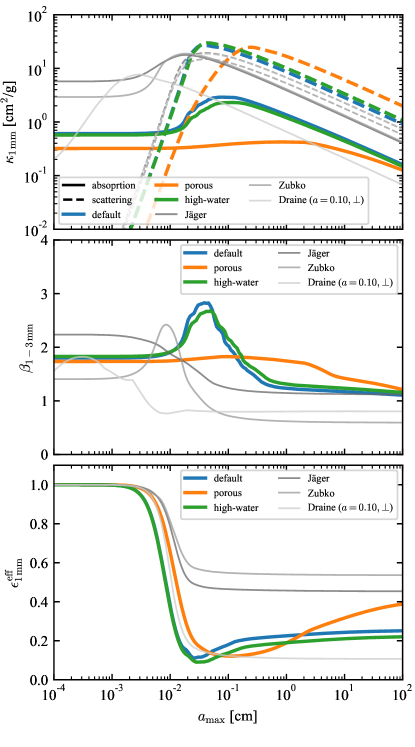
Figure 10: Optical properties for variations in the particle composition. Top panel: absorption (solid lines) and scattering (dashed lines) opacities for different grain models. Middle panel: spectral index in the 1-$3\text{\,}\mathrm{m}\mathrm{m}$ wavelength range. Bottom panel: absorption probability. All properties are calculated for a $q=3.5$ power-law size distribution with variable $a_{\mathrm{max}}$. For description of the models, see Appendix B.

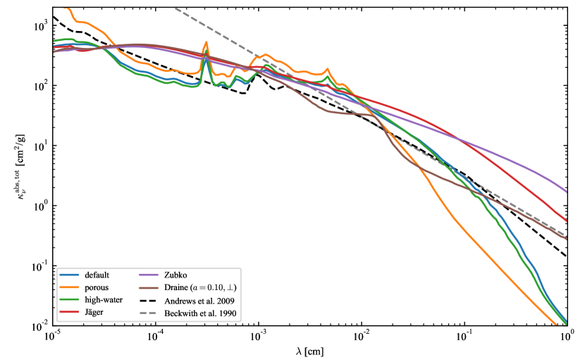
Figure 11: Wavelength dependent absorption opacity of the different grain models discussed in Appendix B averaged over a size distribution up to $a_{\mathrm{max}}=$1\text{\,}\mathrm{m}\mathrm{m}$$. The dashed lines are literature models from Andrews et al. (2009) (black line) and Beckwith et al. (1990) (grey line). For description of the other models, see Appendix B.

References

- ALMA Partnership et al. (2015) ALMA Partnership, Brogan, C. L., Pérez, L. M., et al. 2015, ApJL, 808, L3
- Andrews et al. (2009) Andrews, S. M., Wilner, D. J., Hughes, A. M., Qi, C., & Dullemond, C. P. 2009, ApJ, 700, 1502
- Andrews et al. (2016) Andrews, S. M., Wilner, D. J., Zhu, Z., et al. 2016, ApJL, 820, L40
- Astropy Collaboration et al. (2013) Astropy Collaboration, Robitaille, T. P., Tollerud, E. J., et al. 2013, A&A, 558, A33
- Avenhaus et al. (2018) Avenhaus, H., Quanz, S. P., Garufi, A., et al. 2018, ApJ, 863, 44
- Beckwith & Sargent (1991) Beckwith, S. V. W., & Sargent, A. I. 1991, ApJ, 381, 250
- Beckwith et al. (1990) Beckwith, S. V. W., Sargent, A. I., Chini, R. S., & Guesten, R. 1990, AJ, 99, 924
- Begemann et al. (1994) Begemann, B., Dorschner, J., Henning, T., Mutschke, H., & Thamm, E. 1994, ApJ, 423, L71
- Birnstiel (2018) Birnstiel, T. 2018, dsharp_opac: The DSHARP Mie-Opacity Library, v1.1.0, Zenodo, doi:10.5281/zenodo.1495277. https://doi.org/10.5281/zenodo.1495277
- Birnstiel et al. (2015) Birnstiel, T., Andrews, S. M., Pinilla, P., & Kama, M. 2015, ApJL, 813, L14
- Birnstiel et al. (2010) Birnstiel, T., Dullemond, C. P., & Brauer, F. 2010, A&A, 513, A79
- Birnstiel et al. (2011) Birnstiel, T., Ormel, C. W., & Dullemond, C. P. 2011, A&A, 525, A11
- Bohren & Huffman (1998) Bohren, C. F., & Huffman, D. R. 1998, Absorption and Scattering of Light by Small Particles, 544
- Boudet et al. (2005) Boudet, N., Mutschke, H., Nayral, C., et al. 2005, ApJ, 633, 272
- Brauer et al. (2008) Brauer, F., Dullemond, C. P., & Henning, T. 2008, A&A, 480, 859
- Brown et al. (2009) Brown, J. M., Blake, G. A., Qi, C., et al. 2009, ApJ, 704, 496
- Campbell & Ulrichs (1969) Campbell, M. J., & Ulrichs, J. 1969, J. Geophys. Res., 74, 5867
- Casassus et al. (2013) Casassus, S., Van Der Plas, G., M, S. P., et al. 2013, Nature, 493, 191
- Coupeaud et al. (2011) Coupeaud, A., Demyk, K., Meny, C., et al. 2011, A&A, 535, 124
- D’Alessio et al. (2001) D’Alessio, P., Calvet, N., & Hartmann, L. 2001, ApJ, 553, 321
- D’Alessio et al. (2006) D’Alessio, P., Calvet, N., Hartmann, L., Franco-Hernández, R., & Servín, H. 2006, ApJ, 638, 314
- Demyk et al. (2017) Demyk, K., Meny, C., Lu, X.-H., et al. 2017, A&A, 600, A123
- Demyk et al. (2017a) Demyk, K., Meny, C., Leroux, H., et al. 2017a, A&A, 606, A50
- Demyk et al. (2017b) Demyk, K., Meny, C., Lu, X. H., et al. 2017b, A&A, 600, A123
- Dohnanyi (1969) Dohnanyi, J. S. 1969, J. Geophys. Res., 74, 2531
- Draine (2003) Draine, B. T. 2003, ARA&A, 41, 241
- Draine (2006) —. 2006, ApJ, 636, 1114
- Dullemond & Dominik (2005) Dullemond, C. P., & Dominik, C. 2005, A&A, 434, 971
- Espaillat et al. (2010) Espaillat, C., D’Alessio, P., Hernández, J., et al. 2010, ApJ, 717, 441
- Fedele et al. (2017) Fedele, D., Carney, M., Hogerheijde, M. R., et al. 2017, A&A, 600, A72
- Fedele et al. (2018) Fedele, D., Tazzari, M., Booth, R., et al. 2018, A&A, 610, A24
- Fromang & Nelson (2009) Fromang, S., & Nelson, R. P. 2009, A&A, 496, 597
- Guilloteau et al. (2011) Guilloteau, S., Dutrey, A., Piétu, V., & Boehler, Y. 2011, A&A, 529, 105
- Güttler et al. (2010) Güttler, C., Blum, J., Zsom, A., Ormel, C. W., & Dullemond, C. P. 2010, A&A, 513, 56
- Henning & Stognienko (1996) Henning, T., & Stognienko, R. 1996, A&A, 311, 291
- Huang et al. (2018) Huang, J., Andrews, S. M., Cleeves, L. I., et al. 2018, ApJ, 852, 122
- Hudgins et al. (1993) Hudgins, D. M., Sandford, S. A., Allamandola, L. J., & Tielens, A. G. G. M. 1993, ApJS, 86, 713
- Hunter (2007) Hunter, J. D. 2007, Computing In Science & Engineering, 9, 90
- Isella et al. (2010) Isella, A., Carpenter, J. M., & Sargent, A. I. 2010, ApJ, 714, 1746
- Isella et al. (2016) Isella, A., Guidi, G., Testi, L., et al. 2016, Phys. Rev. Lett., 117, 643
- Ishimaru (1978) Ishimaru, A. 1978, Wave propagation and scattering in random media. Volume I - Single scattering and transport theory (Academic Press)
- Jäger et al. (1998) Jäger, C., Mutschke, H., & Henning, T. 1998, A&A, 332, 291
- Kataoka et al. (2014) Kataoka, A., Okuzumi, S., Tanaka, H., & Nomura, H. 2014, A&A, 568, A42
- Kataoka et al. (2015) Kataoka, A., Muto, T., Momose, M., et al. 2015, ApJ, 809, 78
- Kempf et al. (1999) Kempf, S., Pfalzner, S., & Henning, T. K. 1999, Icarus, 141, 388
- Krijt et al. (2015) Krijt, S., Ormel, C. W., Dominik, C., & Tielens, A. G. G. M. 2015, A&A, 574, A83
- Mathis et al. (1977) Mathis, J. S., Rumpl, W., & Nordsieck, K. H. 1977, ApJ, 217, 425
- Min et al. (2016) Min, M., Rab, C., Woitke, P., Dominik, C., & Ménard, F. 2016, A&A, 585, A13
- Okuzumi et al. (2012) Okuzumi, S., Tanaka, H., Kobayashi, H., & Wada, K. 2012, ApJ, 752, 106
- Ormel & Cuzzi (2007) Ormel, C. W., & Cuzzi, J. N. 2007, A&A, 466, 413
- Ormel & Okuzumi (2013) Ormel, C. W., & Okuzumi, S. 2013, ApJ, 771, 44
- Ormel et al. (2007) Ormel, C. W., Spaans, M., & Tielens, A. G. G. M. 2007, A&A, 461, 215
- Pätzold et al. (2016) Pätzold, M., Andert, T., Hahn, M., et al. 2016, Nature, 530, 63
- Pérez et al. (2012) Pérez, L. M., Carpenter, J. M., Chandler, C. J., et al. 2012, ApJL, 760, L17
- Pérez et al. (2016) Pérez, L. M., Carpenter, J. M., Andrews, S. M., et al. 2016, Science, 353, 1519
- Pinte et al. (2008) Pinte, C., Padgett, D. L., Ménard, F., et al. 2008, A&A, 489, 633
- Pollack et al. (1994) Pollack, J. B., Hollenbach, D., Beckwith, S., et al. 1994, ApJ, 421, 615
- Ricci et al. (2015) Ricci, L., Maddison, S. T., Wilner, D., et al. 2015, ApJ, 813, 138
- Ricci et al. (2010) Ricci, L., Testi, L., Natta, A., et al. 2010, A&A, 512, 15
- Ricci et al. (2012) Ricci, L., Trotta, F., Testi, L., et al. 2012, A&A, 540, 6
- Rybicki & Lightman (1991) Rybicki, G. B., & Lightman, A. P. 1991, Radiative processes in astrophysics
- Shakura & Sunyaev (1973) Shakura, N. I., & Sunyaev, R. A. 1973, A&A, 24, 337
- Tanaka et al. (1996) Tanaka, H., Inaba, S., & Nakazawa, K. 1996, Icarus, 123, 450
- Tazaki & Tanaka (2018) Tazaki, R., & Tanaka, H. 2018, ApJ, 860, 79
- Tazaki et al. (2016) Tazaki, R., Tanaka, H., Okuzumi, S., Kataoka, A., & Nomura, H. 2016, ApJ, 823, 70
- Testi et al. (2003) Testi, L., Natta, A., Shepherd, D. S., & Wilner, D. J. 2003, A&A, 403, 323
- Tsukagoshi et al. (2016) Tsukagoshi, T., Nomura, H., Muto, T., et al. 2016, ApJL, 829, L35
- van der Marel et al. (2013) van der Marel, N., van Dishoeck, E. F., Bruderer, S., et al. 2013, Science, 340, 1199
- Van Der Walt et al. (2011) Van Der Walt, S., Colbert, S. C., & Varoquaux, G. 2011, Computing in Science Engineering, 13, 22
- Warren (1984) Warren, S. G. 1984, Applied Optics, 23, 1206
- Warren & Brandt (2008) Warren, S. G., & Brandt, R. E. 2008, J. Geophys. Res., 113, D13203
- Weidenschilling (1984) Weidenschilling, S. J. 1984, Icarus, 60, 553
- Wilner et al. (2005) Wilner, D. J., D’Alessio, P., Calvet, N., Claussen, M. J., & Hartmann, L. 2005, ApJ, 626, L109
- Windmark et al. (2012) Windmark, F., Birnstiel, T., Güttler, C., et al. 2012, A&A, 540, A73
- Woitke et al. (2016) Woitke, P., Min, M., Pinte, C., et al. 2016, A&A, 586, A103
- Zsom et al. (2010) Zsom, A., Ormel, C. W., Güttler, C., Blum, J., & Dullemond, C. P. 2010, A&A, 513, 57
- Zubko et al. (1996) Zubko, V. G., Mennella, V., Colangeli, L., & Bussoletti, E. 1996, MNRAS, 282, 1321