Some remarks on the
coincidence set
for the Signorini problem

Abstract

We study some properties of the coincidence set for the boundary Signorini problem, improving some results from previous works by the second author and collaborators. Among other new results, we show here that the convexity assumption on the domain made previously in the literature on the location of the coincidence set can be avoided under suitable alternative conditions on the data.

From two generations of students
to a fabulous teacher and friend now in his retirement:
Baldomero Rubio

AMS Subject Classification: 35J86, 35R35, 35R70, 35B60

Keywords: Signorini problem, coincidence set, location estimates, free boundary problem, contact problems

1 Introduction

In the classical Signorini problem of linear elasticity [24], or boundary obstacle problem, an isotropic, homogeneous and linearly hyperelastic material rests in equilibrium over a rigid foundation. Because the contact zone is an unknown of the problem, estimates on its location and size are of interest in the study of the properties of solutions. In the scalar Signorini problem displacements take place along one dimension only and the equation of conservation of momentum is reduced to Poisson’s equation. The simplified model we shall consider in this paper is the following:

$$\left\{\begin{array}[]{rl}-\Delta u=f&\text{ in }\Omega,\\ \begin{array}[]{c}u\geqslant\psi,\text{ }\partial_{\nu}u\geqslant g\\ (u-\psi)(\partial_{\nu}u-g)=0\end{array}&\text{ on }\Gamma.\end{array}\right.$$

Notice that, although the prototypical model for boundary obstacle problems is the one in elasticity theory, other related models with similar boundary conditions are found for instance in semipermeable membranes (the so called parabolic Signorini problem) or stochastic control (with fractional powers of the Laplacian). See the last series of Remarks at the end of the paper.

We recall that the weak mathematical formulation of the model (what we will refer to as Problem 1) is the following: given an open, bounded set $\Omega\subset\mathbbm{R}^{N}$ with Lipschitz boundary $\Gamma=\partial\Omega$ and functions $\psi\in H^{1/2}(\Gamma),g\in H^{-1/2}(\Gamma)$ and $f\in L^{2}(\Omega)$, find $u\in K_{\psi}:=\left\{v\in H^{1}(\Omega):v\geqslant\psi\text{ on }\Gamma\right\}$ such that

$$a_{0}(u,v-u)\geqslant F(v-u)\text{ for all }v\in K_{\psi}$$ (1)

where

$$a_{0}(u,v):=\int_{\Omega}\nabla u\nabla v\mathrm{d}x\text{ and }F(v):=\int_{\Omega}fv\mathrm{d}x+\langle g,v\rangle_{H^{-1/2}(\Gamma)\times H^{1/2}(\Gamma)}.$$ (2)

Since the bilinear form is not coercive some additional conditions on the data must be introduced. In particular, we must assume the compatibility condition

$$\int_{\Omega}f\mathrm{d}x+\langle g,1\rangle_{H^{-1/2}(\Gamma)\times H^{1/2}(\Gamma)}\leq 0.$$ (3)

Notice that (3) is the one-dimensional equivalent of the general condition for vectorial formulations of the problem considered initially by Fichera [16, p. 81], although there it is given in the equivalent form:

$$\int_{\Omega}\mathbf{f}\cdot\mathbf{r}\mathrm{d}x+\int_{\Gamma}\mathbf{g}\cdot\mathbf{r}\mathrm{d}s_{x}\leq 0$$

for every rigid and admissible displacement $\mathbf{r}$, with equality if and only if $\mathbf{-r}$ is also admissible, i.e. the cone of displacements moving the body away from the obstacle. Equivalently, condition (3) means that rigid displacements separating the body from the obstacle increase the elastic energy.

Existence and uniqueness of solution of a general class of problems including Problem 1 follow from [21, Theorem 5.1] which proves the result for general non-symmetric semicoercive bilinear forms, with uniqueness up to a member of a given subset of the rigid displacements $\mathbf{r}$ satisfying the condition $F(\mathbf{r})=0$ (where $F$ was defined in (2)). In our case, since the unknown is scalar we obtain uniqueness once the compatibility condition is assumed.

The coincidence set for a solution $u\in H^{1}(\Omega)$ is defined as the complement of the open set $\left\{x\in\Gamma:u(x)>\psi(x)\text{ in the sense of }H^{1/2}(\Gamma)\right\}$, i.e.

$$I_{\psi}:=\{x\in\Gamma:u(x)=\psi(x)\}.$$ (4)

Observe that it is not justified to require a priori $g\in H^{1/2}(\Omega)$ since $a_{0}$ is not coercive and the solution may fail to be in $H^{2}(\Omega)$ in very simple cases. See, e.g., [1, Theorem I.10] and [19, p. 617] for some classical counterexamples of cases in which $u\not\in H^{2}(\Omega)$, as well as the results presented in [23] and [3].

A common recourse against the lack of coercivity of the bilinear form is to replace the equation by a new one by introducing an additional regularizing term $\alpha u$ with $\alpha>0$ which makes the proofs of existence and uniqueness straightforward. This is done e.g. in [1, Theorem I.10]. In this case the corresponding problem (which we shall refer to as Problem $\mathbf{\alpha}$) involves the PDE $-\Delta u+\alpha u=f$ which leads to the bilinear form

$$a_{\alpha}(u,v):=\int_{\Omega}\nabla u\nabla v\mathrm{d}x+\alpha\int_{\Omega}uv\mathrm{d}x\text{.}$$

Here, the additional linear term $\alpha u$ makes $a_{\alpha}$ coercive even in the case of no Dirichlet boundary conditions and allows for a standard proof of existence and uniqueness applying Stampacchia’s theorem, [21, Theorem 2.1]. Coercivity also allows the use of Brézis’ regularity result [1, Theorem I.10] stating $u\in H^{2}(\Omega)$ whenever $f\in L^{2}(\Omega)$, making the choice $g\in H^{1/2}(\Gamma)$ adequate. We also note that under additional assumptions on the data, the solution is in $L^{\infty}(\Omega)$ (see, e.g. [1, Theorem I.10] and [20, §5]). See also the monograph [22].

Concerning the estimates on the spatial location of the coincidence set we recall that after Friedman’s pioneering paper [17], the first explicit estimates on the location were given in [8, 13] for Problem $\alpha$ with $g=\psi=0$, under the geometric requirement that $\Omega$ be convex and by assuming that the external force be negative near a sufficiently large part of the boundary $\Gamma$.

In Section 2 we extend the conclusion of the above mentioned papers to Problem 1 (see Theorem 1) while also relaxing their assumptions. Section 3 is devoted to the study of location estimates of the coincidence set when the convexity assumption on $\Omega$ is not made. We provide Example 1 in which the coincidence set is totally identified on a non-convex $\Omega$. Finally, by working with a suitable change of coordinates, we prove the main result of this paper (Theorem 3) in which we obtain some location estimates of the coincidence set without any geometrical assumption on $\Omega$ but instead some regularity condition on $\partial\Omega$.

2 Location estimates for Problem 1

As already mentioned, in [13, Theorem 2] the basic geometrical assumption made for the study of Problem $\alpha$ with $g=\psi=0$ is that the domain $\Omega$ must be convex. In this section we first improve on the aforementioned result by considering Problem 1 (i.e., without any regularization term) for non necessarily vanishing data $g$ and $\psi$. Moreover we shall assume convexity only for parts of $\Omega$ near the boundary on which a suitable balance between the external force, the obstacle and the boundary flux becomes negative. We shall also require $C^{3}$ boundary in order to have a tubular neighborhood of $\partial\Omega$ with a $C^{2}$ parametrization given by $x=x(\xi,s)=\xi+s\nu(\xi)$.

Theorem 1

Let $\Omega$ be an open set in $\mathbbm{R}^{N}$ and assume that the data $f,g$ and $\psi$ lead to a unique solution $u\in H^{1}(\Omega)\cap L^{\infty}(\Omega)$ of Problem 1. Assume that there exist $\epsilon,\delta\geq 0$, a subset $\Gamma_{\epsilon,\delta}\subset\Gamma=\partial\Omega$ of class $C^{3}$, and a tubular semi-neighborhood $V_{\rho}^{-}$ of $\Gamma_{\epsilon,\delta}$ for some $\rho>0$ with

$$\rho\text{ large enough and }V_{\rho}^{-}\subset\overline{\Omega},$$ (5)

such that if $\Psi\in H^{2}(V_{\rho}^{-})$ is a nonnegative extension of $\psi$ to $V_{\rho}^{-}$ (i.e. $\Psi=\psi$ on $\Gamma_{\epsilon,\delta}$) then one has

$$f+\Delta\Psi\leq-\epsilon\text{ on }V_{\rho}^{-},$$

and

$$g-\partial_{\nu}\Psi\leqslant-\delta\text{ \ on \ }\Gamma_{\epsilon,\delta}.$$ (6)

Then, if $\epsilon>0$ and

$$\Omega\cap V_{\rho}^{-}\text{ is a convex set,}$$ (7)

we have the location estimate $\Gamma_{\epsilon,\delta}\subset I_{\psi}$ on the coincidence set of $u$.

We note that, in the case in which $f+\Delta\Psi=0$, by assuming the coincidence set $I_{\psi}$ in the class of regular subsets of $\partial\Omega$, a necessary condition in order to have a positively measured coincidence set is that $\int_{I_{\psi}}g-\partial_{\nu}\Psi\leq 0$ (see e.g. [17]). So, in some sense, Theorem 1 shows that a pointwise balance estimate (6) on a good part of $\partial\Omega$ is enough to identify where the coincidence is taking place.

Proof. We first prove the result for the solutions $\tilde{u}_{\alpha}$ of Problem $\alpha$, for any $\alpha>0.$ Notice that it is enough to prove the conclusion for data, $\psi=0,\widetilde{f}:=f+\Delta\Psi-$ $\alpha\Psi$ and $\tilde{g}:=g-\partial_{\nu}\Psi$. Indeed, we let $\tilde{u}$ be the solution of Problem 1 under these conditions, and readily see that $u:=\tilde{u}+\Psi$ solves the problem with data $f,\psi,g$. Let $x_{0}\in\Gamma_{\epsilon,\delta}$ and, for $\rho>0$, let $V_{\rho}^{-}$ be the tubular semi-neighborhood of $\Gamma_{\epsilon,\delta}$ defined by the $C^{2}$ parametrization

$$x=x(\xi,s)=\xi+s\nu(\xi)\text{, for }\xi\in\Gamma_{\epsilon,\delta},s\in(-\rho,0).$$

Let $\|\widetilde{u}\|_{\infty}\leqslant M$. Define $R:=\min\{\mathop{\mathrm{d}ist}\nolimits(x_{0},\Gamma\backslash\Gamma_{\epsilon,\delta}),\rho,MN\}$ and consider the subset $D:=\Omega\cap B(x_{0},R).$ Define $\partial_{1}D:=\partial D\backslash\Gamma$ and $\partial_{2}D:=\partial D\cap\Gamma\subset\Gamma_{\epsilon,\delta}$ as in Figure 1.

Figure 1: The setting in the proof of Theorem 1.

For some $c>0$ define now in $D$ the function $\overline{u}_{\alpha}(x)=c(2N)^{-1}|x-x_{0}|^{2}$. In $D$ we have

$$-\Delta\overline{u}_{\alpha}+\alpha\overline{u}_{\alpha}=-c+\frac{\alpha c}{2N}|x-x_{0}|^{2}\geqslant-\epsilon\geq\widetilde{f}\text{ in }D,$$

assuming

$$0<c\leq\epsilon.$$

Additionally, on $\partial_{1}D$, from assumption (5) we have

$$\overline{u}_{\alpha}\geqslant\frac{c}{2N}R^{2}\geq M\geqslant\tilde{u}_{\alpha}$$

which holds if

$$R\geq\frac{2NM}{c}.$$

Moreover, since by construction $\overline{u}_{\alpha}$ is non-negative, on the subset of the coincidence set $I^{\alpha}:=I_{0}^{\alpha}\cap\partial_{2}D$ we have $\overline{u}_{\alpha}\geqslant\tilde{u}_{\alpha}$ a.e. $I^{\alpha}$ and thus a.e. on all of $\partial_{1}D\cup I^{\alpha}$. Now, the Signorini conditions imply that it has to be $\partial_{\nu}\widetilde{u}_{\alpha}=\tilde{g}$ over $\partial_{2}D-I^{\alpha}$, and, on the other hand we have

$$\partial_{\nu}\overline{u}_{\alpha}(\xi)=cN^{-1}|\xi-x_{0}|\cos(\nu(\xi),\xi-x_{0})\geqslant-\delta\geqslant\tilde{g}\text{ on }\partial_{2}D$$ (8)

where we used the convexity of $\Omega\cap V_{\rho}^{-}$ (positivity of the cosine) in the first inequality. Then, by the comparison principle applied to the associated problem on the set $D$, with Signorini boundary conditions on $\partial_{2}D$ and with Dirichlet conditions on $\partial_{1}D$ (see, e.g. [1]) we deduce finally that $\tilde{u}_{\alpha}\leqslant\overline{u}_{\alpha}$ in $D$ and that the same inequality holds for the traces, that is:

$$0\leqslant\tilde{u}_{\alpha}\leqslant\frac{c}{2N}|\xi-x_{0}|^{2},\text{ over }\Gamma\cap B(x_{0},R)\text{ (in the sense of }H^{1/2}(\Gamma)\text{)}.$$

Letting $\xi\rightarrow x_{0}$ we conclude that for every $\alpha>0$, $\tilde{u}_{\alpha}(x)=0$ a.e. in $\Gamma_{\epsilon,\delta}$ uniformly (since the estimate on the location of $I^{\alpha}:=I_{0}^{\alpha}\cap\partial_{2}D$ is independent of $\alpha$).

Final step. For $\alpha\rightarrow 0$ we let $\tilde{u}_{\alpha}$ be the solutions with data $\widetilde{f}=0$, $\widetilde{\psi}=0$ and $\tilde{g}$ of Problem $\alpha$. The regularity result mentioned above implies that we have $\|\tilde{u}_{\alpha}\|_{\infty}\leqslant M$ uniformly on $\alpha$. Then, by well known results we have $\tilde{u}_{\alpha}\rightarrow\tilde{u}_{0}$ strongly in $H^{1}(\Omega)$ and therefore $\tilde{u}_{0}=0$ on $\Gamma_{\epsilon,\delta}$. $\Box$

Remark. In fact we can also consider the case $\epsilon=0$ and $\delta=0$ under the assumptions of Theorem 1. Indeed, assume for the moment that we can construct, for some $c>0$, a function $w\in H^{2}(D)$ satisfying

$$\left\{\begin{array}[]{lll}-\Delta w\geq\widehat{\epsilon}&\text{in}&D,\\ w\geqslant 0&\text{in}&\overline{D},\\ w=0&\text{on}&\partial_{1}D,\\ \partial_{\nu}w=-\widehat{\delta}&\text{on}&\partial_{2}D.\end{array}\right.$$

Then, the function $\widehat{v}(x):={\tilde{u}_{\alpha}}(x)-w(x)$ is a solution of Problem $\alpha$ for data $\psi=0,\widehat{f}:=f+\Delta\Psi-$ $\alpha\Psi$ $+\Delta w-\alpha w$ and $\widehat{g}:=\widetilde{g}-\widehat{\delta}$. Taking $w(x)=w(s\nu)=\varphi(s)$ and using the expression of the Laplacian on $V_{\rho}^{-}$ (see, e.g. [18] and [25, §4.3.5, p. 62]), the construction of such a $w$ is reduced to finding $\varphi(s)$ such that

$$\left\{\begin{array}[]{rll}-\varphi^{\prime\prime}(s)-(N-1)H(\xi,s)\varphi^{\prime}(s)&\geqslant&c,\\ \varphi(s)&\geqslant&0\\ \varphi(0)&=&0,\\ \varphi^{\prime}(0)&=&-\delta,\end{array}\right.$$

for $s\in(-R,0)$, where $H(\xi,s)$ denotes the mean curvature of the hypersurface, to a distance $s$ of $\Gamma_{\epsilon,\delta}$, i.e. at points $x=x(\xi,s)=\xi+s\nu(\xi),\ \xi\in\Gamma_{\epsilon,\delta}$. When $\Omega\cap V_{\rho}^{-}$ is a convex set, as required in (7), we have that $H(\xi,s)$ is non-negative and bounded for $R$ small enough depending on this convex part of the boundary and thus $w$ can be made explicit.

3 Sharper estimates and further remarks

One of the main goals of this section is to obtain some sharper location estimates on the coincidence set and to extend the previous results while dispensing with the convexity condition (7) on the tubular semi-neighborhood of $\Gamma_{\epsilon,\delta}$. We start by showing in a concrete example that this goal is not impossible.

Example 1

Let $0<R_{0}<R_{1}$ and define the open ring

$$\Omega:=\{x\in B_{R_{1}}(0)\backslash\overline{B}_{R_{0}}(0)\}$$

with inner boundary $\Gamma_{0}:=\partial B_{R_{0}}(0)$ and outer boundary $\Gamma_{1}:=\partial B_{R_{1}}(0)$. Let $\varepsilon>0$, $R_{\varepsilon}\in(R_{0},R_{1}]$ and $f\in L^{2}(\Omega)\cap L^{\infty}(\Omega)$ be such that

$$f(x)\leqslant-\varepsilon\text{\quad a.e. in\quad}\Omega_{\varepsilon}:=B_{R_{\varepsilon}}(0)\backslash B_{R_{0}}(0),$$

and consider the special formulation of the Signorini problem

$$\left\{\begin{array}[]{rlll}-\Delta u&=&f&\text{ in }\Omega,\\ u&=&0&\text{ on }\Gamma_{1}\end{array}\right.\text{ and }\left\{\begin{array}[]{rlll}\partial_{\nu}u&\geqslant&0&\text{ on }\Gamma_{0},\\ u&\geqslant&0&\text{ on }\Gamma_{0},\\ u\partial_{\nu}u&=&0&\text{ on }\Gamma_{0}.\end{array}\right.$$

Notice that we now do not need the compatibility condition since we have Dirichlet conditions on $\Gamma_{1}$.

We claim that the coincidence set is the whole $\Gamma_{0}$, i.e. $u_{|\Gamma_{0}}\equiv 0$.

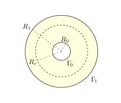
Figure 2: The contact set for a ring is the whole boundary.

To see this we apply again the comparison principle for the associated Problem $\alpha$ for any $\alpha>0$ and then we pass to the limit $\alpha\rightarrow 0$ as in Theorem 1. We define over the ring $\Omega_{\varepsilon}$, the function

$$\overline{u}(x):=c(|x|-R_{0})^{2}$$

for some constant $c>0$ to be determined later. Then, writing $r$ for $|x|$ we have

$$-\Delta\overline{u} = -\frac{d^{2}\overline{u}}{dr^{2}}-\frac{(N-1)}{r}\frac{d\overline{u}}{dr}$$

$$= -2c-\frac{(N-1)}{r}2c(r-R_{0})$$

$$\geqslant -2c\left(1+\frac{N-1}{R_{0}}(R_{\varepsilon}-R_{0})\right).$$

Consequently $-\Delta\overline{u}\geqslant-\varepsilon\geqslant f$ on $\Omega_{\varepsilon}$ whenever $c\leqslant\frac{\varepsilon}{2}\left(1+\frac{N-1}{R_{0}}(R_{\varepsilon}-R_{0})\right)^{-1}$. For instance, we may take $c:=\varepsilon R_{0}/(4NR_{1})$. We set $\overline{f}:=-\Delta\overline{u}$ in $\Omega_{\varepsilon}$ and by construction $\overline{f}\geqslant f$. Let $M:=\|u\|_{\infty,\Omega}$. In order to apply the comparison lemma, we need the condition $\overline{u}\geqslant M$ on $\Gamma_{\varepsilon}:=\partial B_{R_{\varepsilon}}(0)$, that is: $c(R_{\varepsilon}-R_{0})^{2}\geqslant M$ or, equivalently, $R_{\varepsilon}\geqslant R_{0}+\sqrt{M/c}=R_{0}+2(MNR_{1}\varepsilon^{-1}R_{0}^{-1})^{1/2}$ and this is possible for large enough values of $R_{1}$. Furthermore, on $I=\{x\in\Gamma_{0}:u(x)=0\}$ we have $\overline{u}\geqslant u$ too, since by construction $\overline{u}$ is non-negative. Thus $\overline{u}\geqslant u$ on $\Gamma_{\varepsilon}\cup I$ and on the complement $\Gamma_{0}\backslash I$, where $u>0$, the Signorini condition implies $\partial_{\nu}u=0$ and also $\partial_{\nu}\overline{u}=-c(|x|-R_{0})x=0$. Applying the comparison principle we deduce $u\leqslant\overline{u}$ on $\overline{\Omega}_{\varepsilon}$, and in particular $u=0$ over $\Gamma_{0}$.

The following result improves Theorem 1 for the case $\epsilon>0$ and $\delta>0$.

Theorem 2

Assume the conditions of Theorem 1 except condition (7), for some fixed $\epsilon>0$ and $\delta>0$. Then we obtain the location estimate $\Gamma_{\epsilon,\delta}\subset I_{\psi}$ on the coincidence set of $u$.

Proof. We follow the same arguments of the proof of Theorem 1, but instead of condition (7) we use the fact that we can assume that

$$\inf_{x_{0}\in\Gamma_{\epsilon,\delta},x\in V_{\rho}^{-}}\{\cos(x-x_{0},\nu(x_{0})\}\geq-\theta_{0}(\delta,\rho)$$ (9)

for some continuous function $\theta_{0}(\delta,\rho)\geq 0$ (as a matter of fact $\theta_{0}(\delta,\rho)\in[-1,1]$). Then, in (8) we argue instead with

$$\partial_{\nu}\overline{u}_{\alpha}(\xi)=cN^{-1}|\xi-x_{0}|\cos(\nu(\xi),\xi-x_{0})\geqslant-cN^{-1}R\theta_{0}(\delta,\rho)\geqslant-\delta\geq\tilde{g}\text{ on }\partial_{2}D$$

which holds by taking

$$cN^{-1}\theta_{0}(\delta,\rho)R\leq\delta,$$

i.e.

$$c\leq\frac{\delta N}{\theta_{0}(\delta,\rho)R}.$$

Therefore it is enough to take

$$c\leq\min(\epsilon,\frac{\delta N}{\theta_{0}(\delta,\rho)R})$$

and $R\geq\frac{2NM}{c}.$ $\Box$

Remark. Notice that when the tubular semi-neighborhood of $\Gamma_{\epsilon,\delta}$ is convex then $\theta_{0}(\delta,\rho)=0$. We conjecture that, under suitable additional conditions, it should be possible to dispense with at least one of the assumptions $\epsilon>0$ or $\delta>0$ on the semi-neighborhood of $\Gamma_{\epsilon,\delta}$. At present it seems that this fact remains an open problem in the literature. One could try to argue as in the previous Remark in order to extend the result to the case $\epsilon=0$ but with $\delta>0$. However, it is not entirely clear how to construct the function $w$ without condition (7). Notice that in the special case in which we assume that all the mean curvatures $H(\xi,s)$ are constant and equal to $H$, we may actually solve the auxiliary equation of the above Remark without requiring $H\geqslant 0$, but under suitable choices of the interval of definition of such functions. Indeed, the exact solution is given by $\varphi(s)=\varphi_{h}(s)+\varphi_{p}(s)$. For the general solution of the homogeneous equation $\Phi^{\prime}=A\Phi$ with $\Phi=(\varphi,\varphi^{\prime})$, $A=\left(\begin{array}[]{cc}0&1\\ 0&-b\end{array}\right)$ and $b=(N-1)H$ one has $\Phi(s)=\mathrm{e}^{As}\vec{\alpha}$ with $\mathrm{e}^{As}=\left(\begin{array}[]{cc}1&\frac{-1}{b}\mathrm{e}^{-bs}\\ 0&\mathrm{e}^{-bs}\end{array}\right),\vec{\alpha}\in\mathbbm{R}^{2}$. Therefore:

$$\varphi_{h}(s)=\alpha_{1}-\frac{\alpha_{2}}{b}\mathrm{e}^{-bs}.$$

For the particular solution of the inhomogeneous equation we find with the Ansatz $\varphi_{p}(s)=\beta_{1}s^{2}+\beta_{2}s$:

$$\varphi_{p}(s)=\frac{-c}{b}s.$$

Introducing the boundary conditions we arrive at $\alpha_{1}=\alpha_{2}/b=(c/b-\delta)/b$ and

$$\varphi(s)=\left(\frac{c}{b^{2}}-\frac{\delta}{b}\right)(1-\mathrm{e}^{-bs})-\frac{c}{b}s,\quad s\leqslant 0.$$

Finally we have $\varphi(s)\geqslant 0$ over some interval $(-\varepsilon,0)$ because $\varphi^{\prime}$ is continuous and negative at zero, therefore in an interval around it, and $\varphi(0)=0$, meaning that the function decreases to zero from the left.

Our next goal is to improve the location estimates. In order to achieve this we shall not use a function of the Euclidean norm as local supersolution, but a differentiable extension of the intrinsic distance over the manifold $\partial\Omega$. The gradient is then tangent at every point, $\partial_{\nu}\tilde{v}=0$ and we may build simple supersolutions. Let $l(\gamma_{ab})$ denote the length of a piecewise $C^{1}$ curve $\gamma_{ab}$ joining two points $a,b\in\Gamma$. Fix a point $x_{0}\in\Gamma$ and an open neighborhood $\Gamma_{0}$ of $x_{0}$ in $\Gamma$ whose closure is the graph of a Lipschitz map $\varphi:\overline{U}\rightarrow\mathbbm{R}$. Define the intrinsic distance to $\mathbf{x_{0}}$ over $\mathbf{\Gamma}$ as

$$d_{0}(x):=\inf\{l(\gamma_{x_{0}x}):\gamma\in C^{1}([0,1],\Gamma_{0}),\gamma(0)=x_{0},\gamma(1)=x\},x\in\Gamma_{0}$$

With this distance $\overline{\Gamma}_{0}$ is a complete metric space determining the same topology as the differential structure. For $\Gamma_{0}$ smooth enough, $d_{0}$ is a non-negative function in $C^{2}(\Gamma_{0})$ which we now extend. Let $V_{\rho}(\Gamma_{0})$ be a tubular neighborhood of $\Gamma_{0}$ with the $C^{2}$ parametrization

$$x=x(\xi,s)=\xi+s\nu(\xi)\text{ for }\xi\in\Gamma_{0},s\in(-\rho,\rho)$$

and define

$$\tilde{d}_{0}(x)=\tilde{d}_{0}(\xi,s):=[s^{2}+d_{0}(\xi)^{2}]^{1/2}\text{ for every }x\in V_{\rho}(\Gamma_{0}).$$

Now let $V_{0}:=V_{\rho}(\Gamma_{0})\backslash\{x_{0}\}$. The function $\tilde{d}_{0}$ is clearly in $C^{2}(V_{0})$ and we know that

$$\nu(\xi)\text{=-}\nabla\tilde{d}_{0}(\xi)\text{ for any }\xi\in\Gamma_{0}$$ (10)

(see [6, Theorem 8.5, Chapter 7]). Furthermore, for any given $D$ precompact in $V_{0}$, $D\Subset V_{0}$, there exist positive constants $c_{d},C_{d}$ and $c_{\Delta}$ depending on $\tilde{d}$ and $D$ such that

$$c_{d}|x|\leqslant\tilde{d}_{0}(x)\leqslant C_{d}|x|\text{ and }\Delta\tilde{d}_{0}(x)\leqslant c_{\Delta}\text{ for every }x\in D\Subset V_{0}.$$

The second assertion is obvious since $\tilde{d}_{0}\in C^{2}(V_{0})$. For the first simply let $m=\min_{x\in D}\tilde{d}_{0}(x)$, $M=\max_{x\in D}\tilde{d}_{0}(x)$, $l=\min_{x\in D}|x|$, $L=\max_{x\in D}|x|$, where we may assume $l>0$ after a translation placing $x_{0}$ at the origin. Then it suffices to take $c_{d}:=m/L$ and $C_{d}:=M/l$. Finally, using the extension $\tilde{d}_{0}$ we may define for sufficiently small $\tau$ the balls

$$\tilde{B}_{0}(\tau):=\{x\in V_{\rho}(\Gamma_{0}):\tilde{d}_{0}(x)<\tau\}.$$ (11)

Equipped with all this we may finally prove our main result:

Theorem 3

Let $\Omega$ be an open set in $\mathbbm{R}^{N}$ and suppose that the data $f,g$ and $\psi$ lead to a unique solution $u\in H^{1}(\Omega)\cap L^{\infty}(\Omega)$. Assume that there exist $\epsilon,\delta\geq 0$, a subset $\Gamma_{\epsilon,\delta}\subset\partial\Omega$ of class $C^{3}$, and a tubular semi-neighborhood $V_{\rho}^{-}$ of $\Gamma_{\epsilon,\delta}$ equipped with the intrinsic distance, for some $\rho>0$ such that

$$\rho>0\text{ is large enough and }V_{\rho}^{-}\subset\overline{\Omega}$$ (12)

and such that if $\Psi\in H^{2}(V_{\rho}^{-})$ is a nonnegative extension of $\psi$ to $V_{\rho}^{-}$ (i.e. $\Psi=\psi$ on $\Gamma_{\epsilon,\delta}$) then we have that

$$f+\Delta\Psi\leq-\epsilon\text{ on }V_{\rho}^{-},$$

and

$$g-\partial_{\nu}\Psi\leqslant-\delta\text{ \ on \ }\Gamma_{\epsilon,\delta}.$$ (13)

If $\epsilon$ and $\delta$ are strictly positive, then one has the location estimate $\Gamma_{\epsilon,\delta}\subset I_{\psi}$, the coincidence set of $u$.

Proof. As in Theorem 1 it is enough to work with data $\widetilde{f}=f+\Delta\Psi$, $\widetilde{\psi}=0$ and $\tilde{g}:=g-\partial_{\nu}\Psi$. Let $x_{0}\in\Gamma_{\epsilon,\delta}$ and $\rho_{\max}$ the maximal width of a tubular neighborhood around $\Gamma_{\epsilon,\delta}$. Define $R:=\min\{d(x_{0},\Gamma\backslash\Gamma_{\epsilon,\delta}),\rho_{\max}\}$, $D:=\Omega\cap\tilde{B}(x_{0},R)$, $\partial_{1}D:=\partial D\backslash\Gamma$ and $\partial_{2}D:=\partial D\cap\Gamma\subset\Gamma_{\epsilon,\delta}$. Define now in $D$ the function $\overline{u}(x)=cc_{\Delta}^{-1}\tilde{d}_{0}(x)$ for some $c>0$. In $D$ we have

$$-\Delta\overline{u}=-\frac{c}{c_{\Delta}}\Delta\tilde{d}_{0}(x)\geqslant-\epsilon\geq\widetilde{f}.$$

Additionally, on $\partial_{1}D$ we have

$$\overline{u}\geqslant\frac{c}{c_{\Delta}}R\geqslant M\geqslant\tilde{u},$$

assuming that

$$\frac{c}{c_{\Delta}}R\geqslant M.$$

Notice that this condition holds once we take $\rho>0$ (hence also $R$) large enough (for some given $c>0$). Moreover, since $\partial_{\nu}\widetilde{u}=\tilde{g}$ over $\partial_{2}D-I$, by using property (10) we have

$$\partial_{\nu}\overline{u}=cc_{\Delta}^{-1}\partial_{\nu}\tilde{d}_{0}=-cc_{\Delta}^{-1}\geqslant-\delta\geq\tilde{g}\text{ on }\partial_{2}D),$$

once we take

$$cc_{\Delta}^{-1}\leq\delta,$$

i.e.

$$c\leq\min(\delta c_{\Delta},\epsilon).$$

Moreover, since $\overline{u}=0$ in $\partial_{1}D\cup I$ we have $\overline{u}_{\alpha}\geqslant\tilde{u}_{\alpha}$ here. This yields $\tilde{u}\leqslant\overline{u}$ in $H^{1}(D)$ and the same inequality holds for the traces, that is:

$$0\leqslant\tilde{u}(x)\leqslant\frac{c}{c_{\Delta}}\tilde{d}_{0}(x),\text{ over }\Gamma\cap\tilde{B}(x_{0},R)\text{ in }H^{1/2}(\Gamma).$$

Letting $x\rightarrow x_{0}$ we conclude that $\tilde{u}(x)=0$ a.e. in $\Gamma_{\epsilon,\delta}$. $\Box$

4 Final remarks and related work

The above results can be easily extended to the associated heat equation with Signorini boundary conditions by using arguments similar to those found in [12]. Moreover, it is also possible to extend them to Poisson’s equation or to the heat equation with dynamic boundary conditions as in [11] and [7] respectively. Notice that according to the equivalent formulation of the fractional Laplacian operator (see, e.g. [2] and the multiple references given in [10]), the case of dynamical Signorini boundary conditions for the Poisson and related linear equations corresponds to the usual obstacle problem associated to the fractional Laplace operator.

The Signorini boundary conditions can be also formulated in terms of multivalued nonlinear maximal monotone graphs (see [1]). Some results analyzing the set in which the solution vanishes on the boundary for other different nonlinear boundary conditions was the main goal of the paper [14]. See also [4] for the case of singular nonlinear boundary conditions.

The proof techniques used in the present scalar Signorini problem can also be applied to the study of the contact region of one of the vectorial components of the deformation field associated to some problems in linear elasticity (see, e.g., [15] and [5]).

A different class of problems to which the techniques of this paper can be applied are the ones mentioned in the pioneering book [15] concerning temperature control or reverse osmosis membranes (see also the associated homogenization process in [9]).

Miguel de Benito Delgado
University of Augsburg / appliedAI @ UnternehmerTUM GmbH.
m.debenito.d@gmail.com

Jesus Ildefonso Díaz
Instituto de Matemática Interdisciplinar, Universidad Complutense de Madrid.
Plaza de Ciencias 3, 28040 Madrid, Spain.
jidiaz@ucm.es
http://orcid.org/0000-0003-1730-9509

Acknowledgements: The research of the second author was partially supported by the projects with ref. MTM2014-57113-P and MTM2017-85449-P of the DGISPI (Spain).

References

- Brézis [1972] Brézis, H. (1972). Problèmes unilatéraux. Journal de Mathematiques pures et appliquées, (51):1–168.
- Caffarelli and Silvestre [2007] Caffarelli, L. and Silvestre, L. (2007). An Extension Problem Related to the Fractional Laplacian. Communications in Partial Differential Equations, 32(8):1245–1260.
- Caffarelli [1979] Caffarelli, L. A. (1979). Further regularity for the signorini problem. Communications in Partial Differential Equations, 4(9):1067–1075.
- Dávila and Montenegro [2005] Dávila, J. and Montenegro, M. (2005). Nonlinear problems with solutions exhibiting a free boundary on the boundary. Annales de l’I.H.P. Analyse non linéaire, 22(3):303–330.
- de Benito Delgado [2012] de Benito Delgado, M. (2012). Sobre Un Problema de Contacto En Elasticidad. Bachelor’s thesis, Universidad Complutense de Madrid, Madrid.
- Delfour and Zolésio [2011] Delfour, M. and Zolésio, J. (2011). Shapes and Geometries. Advances in Design and Control. Society for Industrial and Applied Mathematics.
- Díaz [2005] Díaz, J. (2005). Special Finite Time Extinction in Nonlinear Evolution Systems: Dynamic Boundary Conditions and Coulomb Friction Type Problems. In Brezis, H., Chipot, M., and Escher, J., editors, Nonlinear Elliptic and Parabolic Problems: A Special Tribute to the Work of Herbert Amann, Progress in Nonlinear Differential Equations and Their Applications, pages 71–97. Birkhäuser Basel, Basel.
- Díaz [1980] Díaz, J. I. (1980). Localización de fronteras libres en inecuaciones variacionales estacionarias dadas por obstáculos. In 3. Congreso de ecuaciones diferenciales y Aplicaciones, pages 1–12, Santiago. Universidad de Santander y Universidad Complutense de Madrid.
- Díaz et al. [2018a] Díaz, J. I., Gómez-Castro, D., Podolskiy, A. V., and Shaposhnikova, T. A. (2018a). Homogenization of a net of periodic critically scaled boundary obstacles related to reverse osmosis “nano-composite” membranes. Advances in Nonlinear Analysis, 0(0).
- Díaz et al. [2018b] Díaz, J. I., Gómez-Castro, D., and Vázquez, J. L. (2018b). The fractional Schrödinger equation with general nonnegative potentials. The weighted space approach. Nonlinear Analysis, 177:325–360.
- Díaz and Jiménez [1985] Díaz, J. I. and Jiménez, R. F. (1985). Aplicación de la teoría no lineal de semigrupos a un operador pseudodiferencial. In Actas del VII CEDYA, pages 137–142, Granada. SEMA.
- Díaz and Jiménez [1986] Díaz, J. I. and Jiménez, R. F. (1986). Behaviour on the boundary of solutions of parabolic equations with nonlinear boundary condition: The evolutionary Signorini problem. In Análisis No Lineal, pages 69–80. PNUD/UNESCO, Univ. de Concepción.
- Díaz and Jiménez [1988] Díaz, J. I. and Jiménez, R. F. (1988). Boundary behaviour of solutions of the Signorini problem. Bolletino U.M.I, 7(2-B):127–139.
- Díaz and Mingazzini [2015] Díaz, J. I. and Mingazzini, T. (2015). Free boundaries touching the boundary of the domain for some reaction–diffusion problems. Nonlinear Analysis: Theory, Methods & Applications, 119:275–294.
- Duvaut and Lions [1976] Duvaut, G. and Lions, J. L. (1976). Inequalities in Mechanics and Physics, volume 219 of Grundlehren der mathematischen Wissenschaften. Springer-Verlag.
- Fichera [1970] Fichera, G. (1970). Unilateral constraints in elasticity. Actes, Congrès international de Mathematiques, 3:79–84.
- Friedman [1967] Friedman, A. (1967). Boundary behavior of solutions of variational inequalities for elliptic operators. Arch. Rational Mech. Anal., 27:95–107.
- Gilbarg and Trudinger [2001] Gilbarg, D. and Trudinger, N. S. (2001). Elliptic Partial Differential Equations of Second Order. Classics in Mathematics. Springer-Verlag, Berlin Heidelberg, 2 edition.
- Kinderlehrer [1981] Kinderlehrer, D. (1981). Remarks about Signorini’s problem in linear elasticity. Annali della scuola normale superiore di Pisa, 8(4):605–645.
- Kinderlehrer and Stampacchia [2000] Kinderlehrer, D. and Stampacchia, G. (2000). An introduction to variational inequalities and their applications, volume 31 of SIAM’s classics in applied mathematics. Society for Industrial and Applied Mathematics, Philadelphia.
- Lions and Stampacchia [1967] Lions, J. L. and Stampacchia, G. (1967). Variational inequalities. Communications on pure and applied mathematics, 20(3):493–519.
- Petrosyan et al. [2012] Petrosyan, A., Shahgholian, H., and Uraltseva, N. (2012). Regularity of Free Boundaries in Obstacle-Type Problems, volume 136 of Graduate Studies in Mathematics. American Mathematical Society.
- Schatzmann [1973] Schatzmann, M. (1973). Problemes aux limites non linéaires non coercifs. Annali della Scuola Normale Superiore di Pisa, CI. Sci. 27, 64:1 – 686.
- Signorini [1959] Signorini, A. (1959). Questioni di elasticità non linearizzata e semilinearizzata. Rendiconti di Matematica e delle sue applicazioni, 18:95–139.
- Sperb [1981] Sperb, R. P. (1981). Maximum Principles and Their Applications. Mathematics in Science and Engineering. Academic Press.