Scaling-Up In-Memory Datalog Processing:
Observations and Techniques

Abstract

Recursive query processing has experienced a recent resurgence, as a result of its use in many modern application domains, including data integration, graph analytics, security, program analysis, networking and decision making. Due to the large volumes of data being processed, several research efforts, across multiple communities, have explored how to scale up recursive queries, typically expressed in Datalog. Our experience with these tools indicated that their performance does not translate across domains—e.g., a tool design for large-scale graph analytics does not exhibit the same performance on program-analysis tasks, and vice versa.

As a result, we designed and implemented a general-purpose Datalog engine, called RecStep, on top of a parallel single-node relational system. In this paper, we outline the different techniques we use in RecStep, and the contribution of each technique to overall performance. We also present results from a detailed set of experiments comparing RecStep with a number of other Datalog systems using both graph analytics and program-analysis tasks, summarizing pros and cons of existing techniques based on the analysis of our observations. We show that RecStep generally outperforms the state-of-the-art parallel Datalog engines on complex and large-scale Datalog program evaluation, by a 4-6X margin. An additional insight from our work is that we show that it is possible to build a high-performance Datalog system on top of a relational engine, an idea that has been dismissed in past work in this area.

1 Introduction

Recent years have seen a resurgence of interest from the research and industry community in the Datalog language and its syntactic extensions. Datalog is a recursive query language that extends relational algebra with recursion, and can be used to express a wide spectrum of modern data management tasks, such as data integration [7, 13], declarative networking [14], graph analysis [20, 21] and program analysis [27]. Datalog offers a simple and declarative interface to the developer, while at the same time allowing powerful optimizations that can speed up and scale out evaluation.

Development of Datalog solvers (or engines) has been a subject of study in both the database community and programming languages community. The database community independently developed its own tools that evaluate general Datalog programs, both in centralized and distributed settings. These include the LogicBlox solver [8], as well as distributed, cloud-based engines such as BigDatalog [23], Myria [24], and Socialite [21].

In programming languages, it has been observed that a rich class of fundamental static program analyses can be written equivalently as Datalog programs [18, 27]. The programming languages community has extensively implemented solvers that target all (or a subset) of Datalog. This line of research has resulted in several Datalog-based tools for program analysis, including the bddbddb [26], Souffle [19], and more recently Graspan [25].

About a year ago, we started exploring the problem of constructing a scalable Datalog engine. We therefore tested Datalog engines from across the two communities. Our experience with these tools indicated that their performance does not translate across domains: Tools such as LogicBlox and bddbddb were unable to scale well with large input datasets prevalent in graph analytics. Even Souffle, the latest and best-performing tool for program analysis tasks, is not well-suited for tasks outside program analysis, such as graph analytics (which also require the language support for aggregation). BigDatalog, Myria, and Socialite, on the other hand, can support only the evaluation of simple Datalog programs with limited recursion capabilities (linear recursion and non-mutual recursion)—however, the majority of program analyses are typically complex Datalog programs with non-linear recursion and mutual recursion.

To address this divide, we asked the following question: Can we design and implement an efficient parallel general-purpose engine that can support a wide spectrum of Datalog programs that target various application domains? In this paper, we answer this question positively, by demonstrating how we can implement a fast in-memory parallel Datalog engine using a relational data management system as a backend. To achieve this goal, we systematically examine the techniques and optimizations necessary to transform a naïve Datalog solver into a highly optimized one that can practically provide efficient large-scale processing. As a consequence of this work, we also show that—contrary to anecdotal and empirical evidence [11]—it is possible to use effectively an rdbms as a backend for Datalog through careful consideration of the underlying system issues.

	Graspan	Bddbddb	BigDatalog	Souffle	RecStep
Scale-Up	yes	no	yes	yes	yes
Scale-Out	no	no	yes	no	no
Memory Consumption	low	low	high	medium	low
CPU Utilization	medium	poor	high	medium	high
CPU Efficiency	low	-	medium	high	high
Hyperparameters Tuning Requried	yes (lightweight)	yes (complex)	yes (moderate)	no	no
Mutual Recursion	yes	yes	no	yes	yes
Non-Recursive Aggregation	no	no	yes	yes	yes
Recursive Aggregation	no	no	yes	no	yes

Table 1: Summary of Comparison Between Different Systems: Here we summarize the comparison of different systems in terms of different aspects. Among these aspects, CPU Efficiency is defined the as the reciprocal of the product of the overall performance (runtime) of the system supporting multi-core computation and the number of CPU cores given for computation - the greater number suggests higher CPU efficiency. We present the formal definition of CPU efficiency and different systems’ CPU efficiency on a few representative workloads in the appendix. The meaning of other aspects should be intuitive as their names suggest.

Our Contribution.

In this paper, we describe the design and implementation of RecStep, a Datalog engine that is built based on our observation and analysis of a set of popular Datalog systems. RecStep is built on top of QuickStep [17], which is a single-node in-memory parallel rdbms and it supports a language extension of pure Datalog with both stratified negation and aggregation, a language fragment that can express a wide variety of data processing tasks.

In more detail, we make the following contributions:

1. Algorithms, data structures, and optimizations: We systematically study the challenges of building a recursive query processing engine on top of a parallel rdbms, and propose a set of techniques that solve them. Key techniques include $(i)$ a lightweight way to enable query re-optimization at every recursive step, $(ii)$ careful scheduling of the queries issued to the rdbms  in order to maximize resource utilization, and $(iii)$ the design of specialized high-performance algorithms that target the bottleneck operators of recursive query processing (set difference, deduplication). We also propose a specialized technique for graph analytics that can compress the intermediate data through the use of a bit-matrix to reduce memory usage. We show how the combination of the above techniques can lead to a high-performance Datalog evaluation engine.

2. Implementation and evaluation: We demonstrate that it is feasible to build a fast general-purpose Datalog engine using an rdbms as a backend. We experimentally show that RecStep can efficiently solve large-scale problems in different domains using a single-node multicore machine with large memory, and also can scale well when given more cores. We perform an extensive comparison of RecStep with several other state-of-the-art Datalog engines on a multi-core machine. We consider benchmarks both from the graph analysis domain (transitive closure, reachability, connected components), and the program analysis domain (points-to and dataflow analyses) using both synthetic and real-world datasets. Our findings show that RecStep outperforms in almost all the cases the other systems, sometimes even by a factor of 8. In addition, the single-node implementation of RecStep compares favorably to cluster-based engines, such as BigDatalog, that use far more resources (more processing power and memory). With the trend towards powerful (multi-core and large main memory) servers, we thus demonstrate that single node systems may be sufficient for a large class of Datalog workloads. The comparison between different systems considering different aspects is summarized in table 1.

Organization. In Section 3, we present the necessary background for Datalog and the algorithms used for its evaluation. Section 4 gives a summary of the architecture design of RecStep, while Section 5 discusses in details the techniques and optimizations that allow us to obtain high-performant evaluation. Finally, in Section 6 we present our extensive experimental evaluation.

2 Related Work

We now compare and contrast our work with existing Datalog engines.

Distributed Datalog Engines. Over the past few years, there have been several efforts to develop a scalable evaluation engine for Datalog. Seo et al. [21] presented a distributed engine for a Datalog variant for social network analysis called Socialite. Socialite employs a number of techniques to enable distribution and scalability, including delta stepping, approximation of results, and data sharding. The notable limitation is Socialite’s reliance on user-provided annotations to determine how to decompose data on different machines. Wang et al. [24] implement a variant of Datalog on the Myria system [9], focusing mostly on asynchronous evaluation and fault-tolerance. The BigDatalog system [23] is a distributed Datalog engine built on a modified version of Apache Spark. A key enabler of BigDatalog is a modified version of rdds in Apache Spark, enabling fast set-semantic implementation. The BigDatalog work has shown superior results to the previously proposed systems which we discussed above, Myria and Socialite. Therefore, in our evaluation, we focus on BigDatalog for a comparison with distributed implementations. Comparing our work with the above systems, we focus on creating an optimized system atop a parallel in-memory database, instead of a distributed setting. The task of parallelizing Datalog has also been studied in the context of the popular MapReduce framework [2, 3, 22]. Motik et al. [16] provide an implementation of parallel Datalog in main-memory multicore systems.

Datalog Solvers in Program Analysis. Static program analysis is traditionally the problem of overapproximating runtime program behaviors. Since the problem is generally undecidable, program analyses resort to overapproximations of runtime facts of a program. A large and powerful class of program analyses, formulated as context-free language reachability, has been shown to be equivalent to Datalog evaluation. Thus, multiple Datalog engines have been built and optimized specifically for program-analysis tasks. The bddbddb Datalog solver [26] pioneered the use of Datalog in program analysis by employing binary decision diagrams (bdd) to compactly represent the results of program analysis. The idea is that there is lots redundancy in the results of a program analysis, due to overapproximation, that bdds help in getting exponential savings. However, recently a number of Datalog solvers have been used for program analysis that employ tabular representations of data. These include the Souffle solver [19] and the LogicBlox solver [8]. Souffle (which has been shown to outperform LogicBlox [5]) compiles Datalog programs into native, parallel C++ code, which is then compiled and optimized for a specific platform. All of these solvers do not employ a deep form of parallelism that our work exhibits by utilizing a parallel in-memory database. The Graspan engine [25] takes a context-free grammar representation and is thus restricted to binary relations—graphs. However, Graspan employs worklist-based algorithm to parallelize fixpoint computation on a multicore machine. As we show experimentally, however, our approach can outperform Graspan on its own benchmark set.

Other Graph Engines. By now, there are numerous distributed graph-processing systems, like Pregel [15] and Giraph [10]. These systems espouse the think-like-a-vertex programming model where one writes operations per graph vertex. These are restricted to binary relations (graphs); Datalog, by definition, is more general, in that it captures computation over hypergraphs.

3 Background

In this section, we provide the background on the syntax and evaluation strategies of the Datalog language. Then, we discuss the language extensions we use in this work.

3.1 Datalog Basics

A Datalog program $P$ is a finite set of rules. A rule is an expression of the following form:

$$h\mathop{:\!\!-}p_{1},p_{2},\dots,p_{k}.$$

The expressions $h,p_{1},\dots,p_{k}$ are atoms, i.e., formulas of the form $R(t_{1},\dots,t_{\ell})$, where $R$ is a table/relation name (predicate) and each $t_{i}$ is a term that can be a constant or a variable. An atom is a fact (or tuple) when all $t_{i}$ are constants. The atom $h$ is called the head of the rule, and the atoms $p_{1},\dots,p_{k}$ are called the body of the rule. A rule can be interpreted as a logical implication: if the predicates $p_{1},\dots,p_{k}$ are true, then so is the head $h$. We assume that rules are always safe: this means that all variables in the head occur in at least one atom in the body. We will use the lower case $x,y,z,\dots$ to denote variables, and $a,b,c,\dots$ for constants.

The relations in a Datalog program are of two types: idb and edb relations. A relation that represents a base (input) table is called edb (extensional database); edb relations can occur only in the body of a rule. A relation that represents a derived relation is called idb (intentional database), and must appear in the head of at least one rule.

Example 1

Let us consider the task of computing the transitive closure (TC) of a directed graph. We represent the directed graph using a binary relation arc(x,y): this means that there is a directed edge from vertex x to vertex y. Transitive closure can be expressed through the following program with two rules:

$$r_{1}:{\tt tc(x,y)} \mathop{:\!\!-}{\tt arc(x,y)}.$$

$$r_{2}:{\tt tc(x,y)} \mathop{:\!\!-}{\tt tc(x,z),arc(z,y)}.$$

In the above Datalog program, the relation arc is an edb relation (input), and the relation tc is an idb relation (output). The program can be interpreted as follows. The first rule $r_{1}$ (called the base rule) initializes the transitive closure by adding to the initially empty relation all the edges of the graph. The second rule $r_{2}$ is a recursive rule, and produces new facts iteratively: a new fact tc(a,b) is added whenever there exists some constant c such that tc(a,c) is already in the relation (of the previous iteration), and arc(c,b) is an edge in the graph.

Stratification. Given a Datalog program $P$, we construct its dependency graph $G_{P}$ as follows: every rule is a vertex, and an edge $(r,r^{\prime})$ exists in $G_{P}$ whenever the head of the rule $r$ appears in the body of rule $r^{\prime}$. A rule is recursive if it belongs in a directed cycle, otherwise it is called non-recursive. A Datalog program is recursive if it contains at least one recursive rule. For instance, the dependency graph of the program in Example 1 contains two vertices $r_{1},r_{2}$, and two directed edges: $(r_{1},r_{2})$ and $(r_{2},r_{2})$. Since the graph has a self-loop, the program is recursive. A stratification of $P$ is a partition of the rules into strata, where each stratum contains the rules that belong in the same strongly connected component in the dependency graph $G_{P}$. The topological ordering of the strongly connected components also defines an ordering in the strata. In our running example, there exist two strata, $\{r_{1}\},\{r_{2}\}$.

3.2 Datalog Evaluation

Datalog is a declarative query language, and hence there are different algorithms that can be applied to evaluate a Datalog program. Most implementations of Datalog use bottom-up evaluation techniques, which start from the input (edb) tables, and then iteratively apply the rules until no more new tuples can be added in the idb relations, reaching a fixpoint. In the naïve evaluation strategy, the rules are applied by using all the facts produced so far. For our running example, we would initialize the idb relation tc with ${\tt tc}^{0}\leftarrow{\tt arc}$. To compute the $(i+1)$ iteration, we compute ${\tt tc}^{i+1}\leftarrow\pi_{x,y}({\tt tc}^{i}\Join{\tt arc})$. The evaluation ends when ${\tt tc}^{i+1}={\tt tc}^{i}$. The naïve evaluation strategy has the drawback that the same tuples will be produced multiple times throughout the evaluation.

In the semi-naïve evaluation strategy, at every iteration the algorithm uses only the new tuples from the previous iteration to generate tuples in the current iteration. For instance, in the running example, at every iteration $i$, we maintain together with ${\tt tc}^{i}$ the facts that are generated only in the $i$-th iteration (and not previous iterations), denoted by $\Delta{\tt tc}^{i}={\tt tc}^{i}-{\tt tc}^{i-1}$. Then, we compute the $(i+1)$ iteration of tc as ${\tt tc}^{i+1}\leftarrow\pi_{x,y}(\Delta{\tt tc}^{i}\Join{\tt arc})$. The running example is an instance of linear recursion, where each recursive rule contains at most one atom with an idb. However, many Datalog programs, especially in the context of program analysis, contain non-linear recursion, where the body of a rule contains multiple idb atoms. In this case, the $\Delta$ relations are computed by taking the union of multiple subqueries (for more details see [1]).

Semi-naïve evaluation can be further sped up by exploiting the stratification of a Datalog program: the strata are ordered (from lower to higher according to the topological order), and then each stratum is evaluated sequentially, by considering the idb relations of prior strata as edb relations (input tables) in the current stratum. In our implementation of Datalog, we use the semi-naïve evaluation strategy in combination with stratification.

3.3 Negation and Aggregation

In order to enhance the expressiveness of Datalog for use in modern applications, we consider two syntactic extensions: negation and aggregation.

Negation. Datalog is a monotone language, which means that it cannot express tasks where the output can become smaller when the input grows. However, many tasks are inherently non-monotone. To express these tasks, we extend Datalog with a simple form of negation, called stratified negation. In this extension, an atom can be negated by adding the symbol $\neg$ in front of the atom. However, the use of $\neg$ is restricted syntactically, such that an atom $R(t_{1},\dots,t_{\ell})$ can be negated in a rule if $(i)$ $R$ is an edb, or $(ii)$ any rule where $R$ occurs in the head is in a strictly lower stratum.

Example 2

Suppose we want to compute the complement of transitive closure, in other words, the vertex pairs that do not belong in the closure. This task can be expressed by the following Datalog program with stratified negation:

$${\tt tc(x,y)} \mathop{:\!\!-}{\tt arc(x,y)}.$$

$${\tt tc(x,y)} \mathop{:\!\!-}{\tt tc(x,z),arc(z,y)}.$$

$${\tt node(x)} \mathop{:\!\!-}{\tt arc(x,y)}.$$

$${\tt node(y)} \mathop{:\!\!-}{\tt arc(x,y)}.$$

$${\tt ntc(x,y)} \mathop{:\!\!-}{\tt node(x),node(y),\neg tc(x,y)}.$$

Aggregation. We further extend Datalog with aggregation operators. To support aggregation, we allow the terms in the head of the rule to be of the form ${\tt AGG}(x,y,\dots)$, where $x,y,\dots$ are variables in the body of the rule, and AGG is an aggregation operator that can be MIN, MAX, SUM, COUNT, or AVG. We allow aggregation not only in non-recursive rules, but also inside recursion as well, which has been early studied in [12]. In the latter case, one must be careful that the semantics of the Datalog program lead to convergence to a fixpoint; in this paper, we assume that the program given as input always converges ([28] studies how to test this property). As an example of the use of aggregation, suppose that we want to compute for each vertex the number of vertices that are reachable from this vertex. To achieve this, we can simply add to the TC Datalog program of Example 1 the following rule:

$$r_{3}:{\tt gtc(x,COUNT(y))} \mathop{:\!\!-}{\tt tc(x,y)}.$$

We should note here that it is straightforward to incorporate negation and aggregation in the standard semi-naïve evaluation strategy, since our syntactic restrictions guarantee that both are applied only when there is no recursion. Hence, they can easily be encoded in a sql query: negation as difference, and aggregation as group-by plus aggregation.

4 Architecture

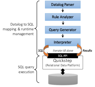
Figure 1: Architectural overview of RecStep

In this section, we present the architecture of RecStep. The core design choice of RecStep is that, in contrast to other existing Datalog engines, it is built on top of an existing parallel in-memory rdbms (QuickStep). This design enables the use of existing techniques (e.g., indexing, memory management, highly optimized operator implementations) that provide high-performance query execution in a multicore environment. Further, it allows us to improve the performance by focusing on characteristics specific to Datalog  evaluation. On the other hand, as we will discuss in more detail in the next section, it creates the challenging problem of reducing the rdbms overhead during execution.

Overview. The architecture of our system is summarized in Figure 1. The Datalog program is read from a .datalog file, which, along with the rules of the Datalog program, provides paths for the input and output tables. The parsed program is first given as input to the rule analyzer. The job of the rule analyzer is to preprocess the program: identify the idb and edb relations (and their mapping to input and output tables), verify the syntactic correctness of the program, and finally construct the dependency graph and stratification. Next, the query generator takes the output of the rule analyzer and produces the necessary sql code to evaluate each stratum of the Datalog program, according to the semi-naïve evaluation strategy. Finally, the interpreter is responsible for the evaluation of the program. It starts the rdbms server, creates the idb and edb tables in the database, and is responsible for the loop control for the semi-naïve evaluation in each stratum. It also controls the communication and flow of information between the rdbms server.

Function	Description
$\mathsf{idb}(s)$	returns relations that are heads in stratum $s$
$\mathsf{rules}(R,s)$	returns rules of stratum $s$ with $R$ as head
$\mathsf{uieval}(r)$	evaluates all the rules in the set $r$
$\mathsf{analyze}(R)$	call to the rdbms to collect statistics for $R$
$\mathsf{dedup}(R)$	deduplicates $R$

Table 2: Notation used in Algorithm 1

Algorithm 1 Execution Strategy for Datalog program $P$

1:for each idb $R$ do

2:     $R\leftarrow\emptyset$

3:end for

4:// $\mathcal{S}$ is a stratification of $P$

5:for each stratum $s\in\mathcal{S}$ do

6:     repeat

7:         for each $R\in\mathsf{idb}(s)$ do

8:              $R_{t}\leftarrow\mathsf{uieval}(\mathsf{rules}(R,s))$

9:              $\mathsf{analyze}(R_{t})$

10:              $R_{\delta}\leftarrow\mathsf{dedup}(R_{t})$

11:              $\mathsf{analyze}(R_{\delta},R)$

12:              $\Delta R\leftarrow R_{\delta}-R$

13:              $R\leftarrow R\uplus\Delta R$

14:         end for

15:         if $s$ is non-recursive then

16:              break

17:         end if

18:     until $\forall R\in\mathsf{idb}(s)$, $\Delta R=0$

19:end for

Execution. We now delve in more detail in how the interpreter executes a Datalog program, a procedure outlined in Algorithm 1.

The Datalog rules are evaluated in groups and order given by the stratification. The idb relations are initialized so that they are empty (line 2). For each stratum, the interpreter enters the control loop for semi-naïve evaluation. Note that in the case where the stratum is non-recursive (i.e., all the rules are non-recursive), the loop exits after a single iteration (line 15). In each iteration of the loop, two temporary tables are created for each idb $R$ in the stratum: $\Delta R$, which stores only the new facts produced in the current iteration, and a table that stores the result at the end of the previous iteration. These tables are deleted right after the evaluation of the next iteration is finished.

The function uieval executes the sql query that is generated from the query generator based on the rules in the stratum where the relation appears in the head (more details on the next section). We should note here that the deduplication does not occur inside uieval, but in a separate call (dedup). This is achieved in practice by using UNION ALL (simply appending data) instead of UNION.

Finally, we should remark that the interpreter calls the function $\mathsf{analyze}()$ during execution, which tells the backend explicitly to collect statistics on the specified table. As we will see in the next section, $\mathsf{analyze}()$ is a necessary feature to achieve dynamic and lightweight query optimization.

5 Optimizations

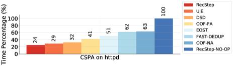
Figure 2: Optimizations for RecStep : Here we show the effects of different optimizations by turning off each optimization of CSPA analysis on httpd dataset . oof-na means the evaluation uses the same query plan at each iteration; oof-fa means collecting all possible data on updated/new tables (idb/intermediate results). RecStep-NO-OP means the evaluation with all optimizations turned off. Regarding the total runtime of RecStep-NO-OP (RecStep with all optimizations turned off) as $100\%$ (time percentage), the runtime of evaluation after turning off each optimization is shown as percentage accordingly.

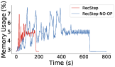
(a) RecStep

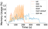
(b) Optimizations

Figure 3: Memory Effects of Optimizations: Here Figure 3 show the memory effect of turning off each optimization of CSPA analysis on httpd, complimenting Figure 2. The memory consumption of RecStep with all optimization turned on/off is shown separately in Figure 3(a) for comparison purpose.

This section presents the key optimizations that we have implemented in RecStep to speed up performance and maximize resource utilization (memory and cores). We consider optimizations in two levels: Datalog-to-sql-level optimizations and system-level optimizations.

For Datalog-to-sql-level optimizations, we study the translation of Datalog rules to a set of corresponding sql queries, so that the evaluation can be done efficiently. This requires careful analysis of the characteristics of the back-end rdbms (QuickStep). Proper translation minimizes the overhead of catalog updates, selects the optimal algorithms and query plans, avoids redundant computations, and fully utilizes the available parallelism.

In terms of system-level optimizations, we focus on those bottlenecks observed in our experiments that cannot be simply resolved by the translation-level optimizations. Instead, we modify the back-end system by introducing new specialized data structures, implementing efficient algorithms, and revising the rules in the query optimizer.

We summarize our optimizations as follows:

1. Unified idb Evaluation (uie): different rules and different subqueries inside each recursive rule evaluating the same idb relation are issued as a single query.

2. Optimization On the Fly (oof): the same set of sql queries are re-optimized at each iteration considering the change of idb tables and intermediate results.

3. Dynamic Set Difference (dsd): for each idb table, the algorithm for performing set-difference to compute $\Delta$ is dynamically chosen at each iteration, by considering the size of idb tables and intermediate results.

4. Evaluation as One Single Transaction (eost): the whole evaluation of a Datalog program is regarded as a single transaction and nothing is committed until the end.

5. Fast Deduplication (fast-dedup): the specialized implementation of global separate chaining hash table exploiting compact key is used for deduplication to speed up the evaluation and use memory more efficiently

Apart from the above list of optimizations, we also provide a specialized technique that can speed up performance on Datalog programs that operate on dense graphs called pbme. This technique represents the relation as a bit-matrix, with the goal of minimizing the memory footprint of the algorithm. We next detail each optimization; their effect on runtime and memory is visualized in Figure 2 and Figure 3. We present the high level analysis of the time and space effect of each optimization in the appendix.

5.1 Datalog-to-SQL-level optimizations

Unified IDB Evaluation (UIE). For each idb relation $R$, there can be several rules where $R$ appears in the head of the rule. In addition, for a nonlinear recursive rule, in which the rule body contains more than one idb relation, the idb relation is evaluated by multiple subqueries. In this case, instead of producing a separate sql query for each rule and then computing the union of the intermediate results, the query generator produces a single sql query using the UNION ALL construct. We call this method unified idb evaluation (uie). Figure 4 provides an example of the two different choices for the case of Andersen analysis.

The idea underlying uie is to fully utilize all the available resources, i.e., all the cores in a multi-core machine. QuickStep does not allow the concurrent execution of sql queries, and hence by grouping the subqueries into a single query, we maximize the number of tasks that can be executed in parallel without explicitly considering concurrent multi-task coordination. In addition, uie mitigates the overhead incurred by each individual query call, and enables the query optimizer to jointly optimize the subqueries (e.g., enable cache sharing, or use pipelining instead of materializing intermediate results). The latter point is not specific to QuickStep, but generally applicable to any rdbms backend (even ones that support concurrent query processing).

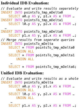
Figure 4: Example uie in Andersen analysis.

Optimization On the Fly (OOF). In Datalog evaluation, even though the set of queries is fixed across iterations, the input data to the queries changes, since the idb relations and the corresponding $\Delta$-relations change at every iteration. This means that the optimal query plan for each query may be different across different iterations.

For example, in some Datalog programs, the size of $\Delta R$ (Algorithm 1) produced in the first few iterations might be much larger than the joining edb table, and thus the hash table should be preferably built on the edb when performing a join. However, as the $\Delta R$ produced in later iterations tend to become smaller, the build side for the hash table should be switched at some point.

In order to achieve optimal performance, it is necessary to re-optimize each query at every iteration (lines 9, 11 in Algorithm 1) by using the latest table statistics from the previous iteration. However, collecting the statistical data (e.g., size, avg, min, max) of the whole database at every iteration can cause a large overhead, since it may be necessary to perform a full scan of all tables. To mitigate this issue, our solution is to control precisely at which point which statistical data we collect for the query optimizer, depending on the type of the query. For instance, before joining two tables, only the size of the two tables is necessary for the optimizer to choose the right side to build the hash table on (the smaller table), as illustrated in the previous example.

In particular, we collect the following statistics:

• For deduplication, the size of the hash table needs to be estimated in order to pre-allocate memory. Instead of computing the number of distinct values in the table (which could be very expensive), we instead use a conservative approximation that takes the minimum of the available memory and size of the table.

• For join processing, we collect only the number of tuples and the tuple size of the joining tables, if any of the tables is updated or newly created.

• For aggregation, we collect statistics regarding the min, max, sum and avg of the tables.

The effect of oof can be seen in Figure 4. Without updating the statistics across the iterations, the running time percentage jumps from $24\%$ to $63\%$ (oof-na). On the other hand, if we update the full set of statistics, the running time percentage increases to $41\%$ (oof-fa). Thus, this optimization provides a $\sim 2.5\textrm{x}$ speedup in the execution time in for the specific program in the experiment.

Dynamic Set-Difference (DSD). In semi-naïve evaluation, the execution engine must compute the set difference between the newly evaluated results ($R_{\delta}$) and the entire recursive relation ($R$) at the end of every iteration, to generate the new $\Delta{R}\leftarrow R_{\delta}-R$ (line 13 in Algorithm 1). Since set difference is executed at every iteration for every idb in the stratum, it is a computational bottleneck that must be highly optimized. There exist two different ways we can translate set difference as a sql query.

The first approach (One-Phase Set Difference – OPSD) simply runs the set difference as a single sql query. The default strategy that QuickStep uses for set difference is to first build a hash table on $R$, and then $R_{\delta}$ probes the hash table to output the tuples of $R_{\delta}$ that do not match with any tuple in the hash table. Since the size of $R$ grows at each iteration (recall that Datalog is monotone), this suggests that the cost of building the hash table on $R$ will constantly increase for the set difference computation under OPSD.

An alternative approach is to use a translation that we call Two-Phase Set Difference (TPSD). This approach involves two queries: the first query computes the intersection of the two relations, $r\leftarrow R\cap R_{\delta}$. The second query performs set difference, but now between $R$ and $r$ (instead of $R_{\delta}$). Although this approach requires more relational operators, it avoids building a hash table on $R$.

We observe that none of the two approaches always dominates the other, since the size of $R$ and $R_{\delta}$ changes at different iterations. Hence, we need to dynamically choose the best translation at every iteration. To guide this choice, we devise a simple cost model. In this model, we assign a (per tuple) build cost $C_{b}$ during the hash table build phase and a probe cost $C_{p}$ during the hash table probe phase. Let $\alpha=C_{b}/C_{p}$ be the ratio of build to probe cost, $\beta=|R|/|R_{\delta}|$ and $\mu=|R_{\delta}|/|r|$. We should note here that $\alpha,\beta$ are known before execution, while the intersection size $|r|$ (and hence $\mu$) is unknown. Based on the cost model, we can calculate that OPSD is chosen when $\beta\in(0,1]$ (i.e., when $R$ is the smallest table), and TPSD is chosen if $\beta\geq\frac{2\alpha}{\alpha-1}$. When $\beta$ lies in $(1,\frac{2\alpha}{\alpha-1})$, the choice depends on $\mu$, whose value we can approximate using the value of $\mu$ from the previous iteration. We present the detailed analysis of the cost model in the appendix.

5.2 System-level Optimizations

Evaluation as One Single Transaction (EOST). By default, QuickStep  (as well as other rdbmss) view each query that changes the state of database as a separate transaction. Keeping the default transaction semantics in QuickStep  during evaluation incurs I/O overhead in each iteration due to the frequent insertion in idb tables, and the creation of tables storing intermediate results. Such frequent I/O actions are unnecessary, since we only need to commit the final results at the end of the evaluation. To avoid this overhead, we use the evaluation as one single transaction (eost) semantics. Under these semantics, the data is kept in memory until the fixpoint is reached (when there is enough main memory), and only the final results are written to persistent storage at the end of evaluation.

To achieve eost, we slightly modify the kernel code in QuickStep to pend the I/O actions until the fixpoint is reached (by default, if some pages of the table are found dirty after a query execution, the pages are written back to the disk). At the end of the evaluation, a signal is sent to QuickStep and the data is written to disk. For other popular rdbmss (e.g., PostgreSQL, MySQL, SQL Server), the start and the end of a transaction can be explicitly specified, but this approach is only feasible for a set of queries that are pre-determined. However, in recursive query processing the issued queries are dynamically generated, and the number of iterations is not known until the fixpoint is reached, which means that similar changes need to be made in these systems to apply eost.

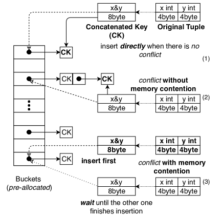
Figure 5: Example of applying fast deduplication algorithm on table with two integer attributes in RecStep 

Fast Deduplication. In Datalog evaluation, deduplication of the evaluated facts is not only necessary for conforming to the set semantics, but also helps to avoid redundant computation. Deduplication is also a computational bottleneck, since it occurs at every iteration for every idb in the stratum (line 10 in Algorithm 1); hence, it is necessary to optimize its parallel execution.

To achieve this, we use a specialized Global Separate Chaining Hash Table implementation that uses a Compact Concatenated Key (ck), which we call cck-gscht. cck-gscht is a global latch-free hash table built using a compact representation of $\langle key,value\rangle$ pairs, in which tuples from each data partition/block can be inserted in parallel. Figure 5 illustrates the deduplication algorithm using an example in which cck-gscht is applied on a table with two integer attributes (src int, dest int).

Based on the approximated number of distinct elements from the query optimizer, we pre-allocate a list of buckets, where each bucket contains only a pointer. An important point here is that the number of pre-allocated buckets will be as large as possible when there is enough memory, for the purpose of minimizing conflicts in the same bucket, and preventing memory contention. Tuples are assigned to each thread in a round-robin fashion and are inserted in parallel. Knowing the length of each attribute in the table, a compact ck of fixed size is constructed for each tuple (8 bytes for two integer attributes as shown in Figure 5). The compact ck itself contains all information of the original tuple, eliminating the need for explicit $\langle key,value\rangle$ pair representation. Additionally, the key itself is used as the hash value, which saves computational cost and memory space.

5.3 Parallel Bit-Matrix Evaluation

Algorithm 2 Parallel Bit-Matrix Evaluation of TC

1:Input: $arc(x,y)$ - edb relation, number of threads $k$

2:Output: $tc(x,y)$ - idb relation

3:// $M_{arc}$: virtual bit-matrix of ${\tt arc(x,y)}$

4:Construct bit-matrix $M_{tc}$ of ${\tt tc(x,y)}$

5:$M_{tc}\leftarrow M_{arc}$

6:Partition the rows of $M_{tc}$ into $k$ partitions

7:// the $k$ threads evaluate $k$ partitions in parallel

8:for each row $i$ in partition $p$ do

9:     $\delta\leftarrow\{u\mid M_{tc}[i,u]=1\}$

10:     while $\delta\neq\emptyset$ do

11:         $\delta_{n}\leftarrow\emptyset$

12:         for each $t\in\delta$  do

13:              for each $j$ s.t. ${M_{arc}}[t,j]=1$ do

14:                  if ${M_{tc}}[i,j]=0$ then

15:                       $\delta_{n}\leftarrow\delta_{n}\cup\{j\}$

16:                       ${M_{tc}}[i,j]\leftarrow 1$

17:                  end if

18:              end for

19:         end for

20:         $\delta\leftarrow\delta_{n}$

21:     end while

22:end for

Algorithm 3 Parallel Bit-Matrix Evaluation of SG

1:Input: ${\tt arc(x,y)}$ - edb relation, number of threads $k$

2:Output: ${\tt tc(x,y)}$ - idb relation

3:// $M_{arc}$: virtual bit-matrix of ${\tt arc(x,y)}$

4:Construct vector index $V_{arc}[x]=\{y$ $|$ $M_{arc}[x,y]=1\}$

5:Construct $M_{sg}$ bit-matrix of ${\tt sg(x,y)}$

6:// ${\tt sg(x,y)}\leftarrow{\tt arc(p,x),arc(p,y),x\leftarrow y.}$

7:// ${\tt arc_{1}}\leftarrow$ $\textbf{Rename}_{arc_{1}(x_{1},y_{1})}({\tt arc})$

8:// ${\tt arc_{2}}\leftarrow$ $\textbf{Rename}_{arc_{2}(x_{2},y_{2})}({\tt arc})$

9:$M_{sg}\leftarrow\Pi_{y_{1},y_{2}}(M_{arc_{1}}\bowtie_{x_{1}=x_{2},y_{1}\neq y_{2}}M_{arc_{2}})$

10:Partition the rows of $M_{sg}$ into $k$ partitions

11:// $k$ threads evaluate $k$ partitions in parallel

12:for each row $i$ in partition $p$ do

13:     $\delta\leftarrow\{(i,u)\mid{M_{sg}}[i,u]=1\}$

14:     while $\delta\neq\emptyset$ do

15:         $\delta_{n}\leftarrow\emptyset$

16:         for each $(a,b)\in\delta$ do

17:              for each $q\in{V_{arc}}[a]$ do

18:                  for each $p\in{V_{arc}}[b]$ do

19:                       if ${M_{sg}[q,p]}=0$ then

20:                           $\delta_{n}\leftarrow\delta_{n}\cup\{(q,p)\}$

21:                           $M_{sg}[q,p]\leftarrow 1$

22:                       end if

23:                  end for

24:              end for

25:         end for

26:         $\delta\leftarrow\delta_{n}$

27:     end while

28:end for

In our experimental evaluation, we observed that the usage of memory increases drastically during the evaluation of graph analytics over dense graphs. By default, QuickStep uses hash tables for joins between tables, aggregation and deduplication. When the intermediate result becomes very large, the use of hash tables for join processing becomes memory-costly. In the extreme, the intermediate results are too big to fit in main memory, and are forced to disk, incurring additional I/O overhead. This can cause in the worst case scenario out-of-memory errors (oom). Additionally, the materialization cost of large intermediate results can hurt performance.

Besides graph analytics on dense graphs, in many program analyses idb relations, even though they can be large, they are very dense and the active domain of the relational attributes is relatively smaller. This phenomenon is also observed in dense graph analytics, where graphs with a small number of vertices produce results that are a orders of magnitude larger than the inputs.

Inspired by this observation, we exploit a specialized data structure, called bit-matrix, that replaces a hash map during join and deduplication in the case when the graph representing the data is dense and has relatively small number of vertices. This data structure represents the join results in a much more compact way under certain conditions, greatly reducing the memory cost compared to a hash table (The comparison of memory consumption before using PBME and after in TC and SG is visualized in Figure 6). In this paper, we only describe the bit matrix for binary relations, but we note that the technique can be extended to relations of higher arity. At the same time, we implement new operators directly operating on the bit-matrix, naturally merging the join and deduplication into one single stage and thus avoid the materialization cost coming from the intermediate results. We call this technique Parallel Bit-Matrix Evaluation (pbme). In our experiments, pbme provided a huge boost in performance for transitive closure (TC) and same generation (SG).

We next describe the bit-matrix technique and present two examples in which it is used for evaluation of TC and SG as outlined in Algorithm 2 and Algorithm 3. Note that we construct a matrix only for each idb, but for convenience of illustration, we use matrix notation for the edbs as well (line 3 in Algorithm 2 and Algorithm 3).

The Bit-Matrix Data Structure. Let $R(x,y)$ be a binary idb relation, with active domain $\{1,2,\dots,n\}$ for both attributes. Instead of representing $R$ as a set of tuples, we represent it as an $n\times n$ bit matrix denoted $M_{R}$. If $R(a,b)$ is a tuple in $R$, the bit at the $a$-th row and $b$-th column, denoted ${M_{R}}[a,b]$ is set to 1, otherwise it is 0. The relation is updated during recursion by setting more bits from 0 to 1. We decide to build the bit-matrix data structure only if the memory available can fit both the bit matrix, as well as any additional index data structures used during evaluation (e.g., Algorithm 3).

One of the key features of pbme is zero-coordination: each thread is only responsible for the partition of data assigned to it and there is no or nearly no coordination needed between different threads. Algorithm 2 outlines the pbme for transitive closure. For the evaluation of TC (Algorithm 2), the rows of the idb bit-matrix $M_{tc}$ are firstly partitioned in a round-robin fashion (line 6). For each row $i$ assigned to each thread, the set $\delta$ stores the new bits (paths starting from $i$) produced at every iteration (line 12-19). For each new bit $t$ produced, the thread searches for all the bits at row $t$ of $M_{arc}$, and computes the new $\delta$ (line 13-19).

The Datalog program of SG is as follows:

$${\tt sg(x,y)} \mathop{:\!\!-}{\tt arc(p,x),arc(p,y),x!=y}.$$

$${\tt sg(x,y)} \mathop{:\!\!-}{\tt arc(a,x),sg(a,b),arc(b,y)}.$$

The pbme of SG is outlined in Algorithm 3, and has some differences compared to that of TC. In addition to the output matrix, an additional index is built on the edb relation ${\tt arc{(x,y)}}$ (line 4), since the edb relation ${\tt arc{(x,y)}}$ appears twice in the recursive rule, direct scanning the edb tables without using index (line 17-18 uses index scan) might introduce great amount of redundant computation. Unlike evaluation of TC, we note that issues such as data skew and redundant computation for SG are possibly seen in evaluation of different threads in different data partitions mainly because $\delta$ (Algorithm 3 line 20 -21) in Algorithm 3 produced is not tied to data partitions assigned to threads (in TC, each row $i$ in partition $p$ always updates the bit in row $i$, a.k.a $M_{tc}[i,]$ - Algorithm 2 line 13). To analyze the effect of data skew, we implement an experimental SG-PBME with coordination (SG-PBME-COORD) and compare it with SG-PBME without coordination as shown in Figure 7. SG-PBME-COORD mitigates the data skew by aggregating and re-balancing - when a thread has generated $\delta$ the size of which is above a given threshold $t$, the $\delta$ is aggregated and packed as a work order, being sent to the global pool. Threads that are idle will grab work orders from the global pool to achieve load balancing. There is a trade-off incurred by the choice of $t$ - if $t$ is too small, then there will be too much communication overheads incurred by message passing, slowing down the performance; on the contracy, if $t$ is too large, then workload balancing cannot be well achieved when the skew is serious. Meanwhile, coordination will only incur unnecessary overhead when there is nearly no skew in data. We leave all the detailed analysis and study of this coordination approach in our future work.

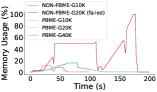
(a) Transitive Closure

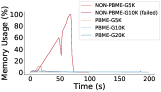
(b) Same Generation

Figure 6: Memory Saving of PBME on TC and SG)

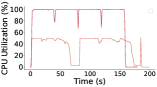
(a) CPU Utilization

(b) Memory Usage

Figure 7: (G20K) SG-PBME Coordination v.s Non-Coordination: As shown in Figure 7(a), with proper coordination, the CPU utilization of PBME with coordination achieves almost $100\%$ throughout the whole evaluation of SG on G20k and it takes less time to finish compared to PBME without coordination. There is no much difference in memory consumption of two methods as shown in Figure 7(b).

6 Experimental Evaluation

In this section, we evaluate the performance of RecStep. Our experimental evaluation focuses on answering the following two questions:

1. How does our proposed system scale with increased computation power (cores) and data size?

2. How does our proposed system perform compared to other parallel Datalog evaluation engines?

To answer these two questions, we perform experiments using several benchmark Datalog programs from the literature: both from traditional graph analytics tasks (e.g., reachability, shortest path, connected components), as well as program analysis tasks (e.g., pointer static analysis). We compare RecStep against a variety of state-of-the-art Datalog engines, as well as a recent single-machine, multicore engine (Graspan), which can express only a subset of Datalog.

6.1 Experimental Setup

We briefly describe here the setup for our experiments.

System Configuration. Our experiments are conducted on a bare-metal server in Cloudlab [6], a large cloud infrastructure. The server runs Ubuntu 14.04 LTS and has two Intel Xeon E5-2660 v3 2.60 GHz (Haswell EP) processors. Each processor has 10 cores, and 20 hyper-threading hardware threads. The server has 160GB memory and each NUMA node is directly attached to 80GB of memory.

Other Datalog Engines. We compare the performance of RecStep with several state-of-the-art systems that perform either general Datalog evaluation, or evaluate only a fragment of Datalog for domain-specific tasks.

1. BigDatalog [23] is a general-purpose distributed Datalog system implemented on top of Spark.

2. Souffle [19] is a parallel Datalog evaluation tool that compiles Datalog to a native C++ program. It focuses on evaluating Datalog programs for the domain of static program analysis.

3. bddbddb [26] is a single-thread Datalog solver designed for static program analysis. Its key feature is the representation of relations using binary decision diagrams (bdds).

4. Graspan [25] is a single-machine disk-based parallel graph system, used mainly for interprocedural static analysis of large-scale system code.

Graph Analytics	Datasets	Reference
Transitive Closure (TC)	[G5K, G10K, G10K-0.01, G10K-0.1, G20K, G40K, G80K]	[23]
Same Generation (SG)	[G5K, G10K, G10K-0.01, G10K-0.1, G20K, G40K, G80K]	[23]
Reachability (REACH)	[livejournal, orkut, arabic, twitter], RMAT	[23]
Connected Components (CC)	[livejournal, orkut, arabic, twitter], RMAT	[23]
Single Source Shortest Path (SSSP)	[livejournal, orkut, arabic, twitter], RMAT	[23]
Program Analysis	Datasets	Reference
Andersen’s Analysis (AA)	7 synthetic datasets	-
Context-sensitive Dataflow Analysis (CSDA)	[linux, postgresql, httpd]	[25]
Context-sensitive Points-to Analysis (CSPA)	[linux, postgresql, httpd]	[25]

Table 3: Summary of Datalog Programs and Datasets in Performance Evaluation

6.2 Benchmark Programs and Datasets

We conduct our experiments using Datalog programs that arise from two different domains: graph analytics and static program analysis. The graph analytics benchmarks are those used for evaluating BigDatalog [23]. Below, we present them in detail (with the exception of TC and SG, which are described earlier in the paper).

Reachability

$${\tt reach(y)} \mathop{:\!\!-}{\tt id(y)}.$$

$${\tt reach(y)} \mathop{:\!\!-}{\tt reach(x),arc(x,y)}.$$

Connected Components

$${\tt cc3(x,MIN(x))} \mathop{:\!\!-}{\tt arc(x,\_)}.$$

$${\tt cc3(y,MIN(z))} \mathop{:\!\!-}{\tt cc3(x,z),arc(x,y)}.$$

$${\tt cc2(x,MIN(y))} \mathop{:\!\!-}{\tt cc3(x,y)}.$$

$${\tt cc(x)} \mathop{:\!\!-}{\tt cc2(\_,x)}.$$

Single Source Shortest Path

$${\tt sssp2(y,MIN(0))} \mathop{:\!\!-}{\tt id(y)}.$$

$${\tt sssp2(y,MIN(d1+d2))} \mathop{:\!\!-}{\tt sssp2(x,d1),arc(x,y,d2)}.$$

$${\tt sssp(x,MIN(d))} \mathop{:\!\!-}{\tt sssp2(x,d)}.$$

The static analysis benchmarks include analyses on which Graspan was evaluated [25], as well as a classic static analysis called Andersen’s analysis [4].

Andersen’s Analysis

$${\tt pointsTo(y,x)} \mathop{:\!\!-}{\tt addressOf(y,x)}.$$

$${\tt pointsTo(y,x)} \mathop{:\!\!-}{\tt assign(y,z),pointsTo(z,x)}.$$

$${\tt pointsTo(y,w)} \mathop{:\!\!-}{\tt load(y,x),pointsTo(x,z),pointsTo(z,w)}.$$

$${\tt pointsTo(z,w)} \mathop{:\!\!-}{\tt store(y,x),pointsTo(y,z),pointsTo(x,w)}.$$

Context-sensitive Points-to Analysis (CSPA)

$${\tt valueFlow(y,x)} \mathop{:\!\!-}{\tt assign(y,x)}.$$

$${\tt valueFlow(x,y)} \mathop{:\!\!-}{\tt assign(x,z),memoryAlias(z,y)}.$$

$${\tt valueFlow(x,y)} \mathop{:\!\!-}{\tt valueFlow(x,z),valueFlow(z,y)}.$$

$${\tt memoryAlias(x,w)} \mathop{:\!\!-}{\tt dereference(y,x),valueAlias(y,z)},$$

$${\tt dereference(z,w)}.$$

$${\tt valueAlias(x,y)} \mathop{:\!\!-}{\tt valueFlow(z,x),valueFlow(z,y)}.$$

$${\tt valueAlias(x,y)} \mathop{:\!\!-}{\tt valueFlow(z,x),memoryAlias(z,w)},$$

$${\tt valueFlow(w,y)}.$$

$${\tt valueFlow(x,x)} \mathop{:\!\!-}{\tt assign(x,y)}.$$

$${\tt valueFlow(x,x)} \mathop{:\!\!-}{\tt assign(y,x)}.$$

$${\tt memoryAlias(x,x)} \mathop{:\!\!-}{\tt assign(y,x)}.$$

$${\tt memoryAlias(x,x)} \mathop{:\!\!-}{\tt assign(x,y)}.$$

Context-sensitive Dataflow Analysis (CSDA)
(uses results of CSPA)

$${\tt null(x,y)} \mathop{:\!\!-}{\tt nullEdge(x,y)}.$$

$${\tt null(x,y)} \mathop{:\!\!-}{\tt null(x,w)},{\tt arc(w,y)}.$$

To evaluate the benchmark programs, we use a combination of synthetic and real-world datasets, which are summarized in Table 3. To give a better view of the performance evaluation, we briefly summarize some of the datasets and corresponding Datalog programs here. For more details, readers can go to the reference.

G$n$-$p$ graphs are graphs generated by the GTgraph synthetic graph generator, where $n$ represents the number of total vertices of the graph in which each pair of vertices is connected by probability $p$. Each pair of vertices in G$n$ omitting $p$ is connected with probability $0.001$. All G$n$-$p$ graphs are very dense considering their relatively small number of vertices. SG and TC generate very large results when evaluation is performed on G$n$-$p$, (at least a few orders of magnitude larger than the number of vertices). RMAT graphs are graphs generated by the RMAT graph generator, with the same specification in [23], RMAT-n represents the graph that has $n$ vertices and 10$n$ directed edges ($n\in{1M,2M,4M,8M,16M,32M,64M,128M}$ in our evaluation experiments). livejournal, orkut, arabic, twitter are all large-scale real-world graphs which have tens of millions of vertices and edges. For the Andersen analysis, seven datasets are generated ranging from small size to large size based on the characteristics of a tiny real dataset available at hand, numbered from 1 to 7. The graph representations of the datasets are small and produce moderate number of tuples. linux, postgresql, httpd are all real system programs used for CSDA and CSPA experiments in [25].

6.3 Experimental Results

We first evaluate the scalability of our proposed engine, and then move to a comparison with other systems.

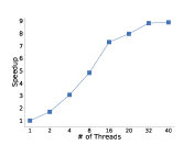
(a) CSPA on httpd

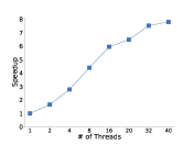
(b) CC on livejournal

Figure 8: Scaling-up on Cores

Scaling-up Cores. To evaluate the speedup of RecStep, we run the CC benchmark on livejournal graph, and the CSPA benchmark on the httpd dataset. We vary the number of threads from 2 to 40. Figure 8 demonstrates that for both cases, RecStep scales really well using up to 16 threads, and after that point achieves a much smaller speedup. This drop on speedup occurs because of the synchronization/scheduling primitive around the common shared hash table that is accessed from all the threads. Recall that 20 is the total number of physical cores.

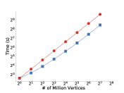
(a) CC on RMAT

(b) AA on synthetic dataset

Figure 9: Scaling-up on Datasets: the x-axis of 9(a) represents the number of vertices of the corresponding RMAT graph datasets (RMAT-1M to RMAT-128M); the synthetic datasets are numbered from 1 to 7 and the x-axis of 9(b) suggests the corresponding dataset number.

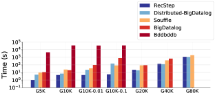
(a) Transitive Closure

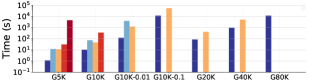
(b) Same Generation

Figure 10: Performance Comparison of TC and SG

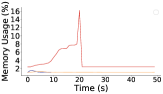
(a) Transitive Closure

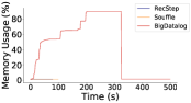
(b) Same Generation

Figure 11: Memory Usage of TC and SG (G10k)

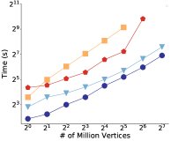
(a) REACH

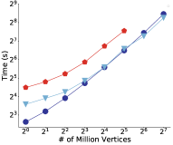
(b) CC

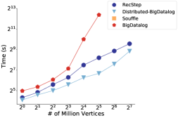
(c) SSSP

Figure 12: Performance Comparison on RMAT Graphs: The x-axis represents RMAT-1M to RMAT-128M.

Scaling-up Data. We perform experiments on both a graph analytics program (CC on RMAT) and a program analysis task (AA on the synthetic datasets) using all 20 physical cores (40 hyperthreads) to observe how our system scales over datasets of increasing sizes. From Figure 9(a), we observe the time increases nearly proportionally to the increasing size of the datasets. In Figure 9(b), we observe that for datasets numbered from 1 to 3, the evaluation times on these three datasets are roughly the same. The corresponding graphs representing the input for these three datasets are relatively sparse and the total size of the data (input and intermediate results) during evaluation is small, and the cores/threads are underutilized; thus, when the data increases, the stale threads will take over the extra processing, and runtime will not increase. With the increasing size of datasets (4 to 7), we observe a similar trend as seen in Figure 9(a) since the size of input data as well as that of the produced intermediate results increases. All cores are fully utilized, so more data will cause increase in runtime.

Comparison With Other Systems. In this section, we report experimental results over our benchmarks for several other Datalog systems and Graspan. For each Datalog program and dataset shown in the comparison results, we run the evaluation four times (with the exception of bddbddb, since its runtime is substantially longer than all other systems across the workloads), we discard the first run and report the average time of the last three runs. For each system, we report the total execution time, including the time to load data from the disk and write data back to the disk. For BigDatalog, since its evaluation is parameter workload dependent based on the available resources provided (e.g., memory), and its performance depends on both of the supplied parameters, datasets and the programs, we tried different combinations of parameters (e.g., different join types) and report the best runtime numbers. For comparison purpose, we also display the results of BigDatalog that runs on the full cluster from [23] (Distributed-BigDatalog in Figure 10, 12, 13, which has $15$ worker nodes with 120 CPU cores and 450GB memory in total). As we will see next, the experiments show that our system can efficiently evaluate Datalog programs for both large-scale graph analytics and program analyses, by being able to efficiently utilize the available resources on a single node equipped with powerful modern hardware (multi-core processors and large memory). Specific runtime numbers are not shown in Figure 10 and Figure 15(a) due to the space limit.

TC and SG Experiments. For TC and SG, our system uses pbme as discussed in Section 5. Since the G$n$-$p$ graphs are very dense, in each iteration intermediate results of large sizes are produced. Hence, the original QuickStep operators run out of memory due to the high materialization cost and demand for memory. By using a bit-matrix data structure, the evaluation naturally fuses the join and deduplication into a single computation, avoiding the materialization cost and heavy memory usage. Our system is the only one that can complete the evaluation for TC and SG on all G$n$-$p$ graphs (the runtime bar is not shown if the system fails to finish the evaluation due to OOM or timeout ($>10h$) is observed ). The evaluation time of all four systems is shown in Figure 10 and Figure 11 shows the memory consumption of each system.

For TC, except for Distributed-BigDatalog, our system outperforms all other systems on all G$n$-$k$ graphs (Distributed-BigDatalog is only slightly faster than RecStep  on G20K, G40K and G80K). For G5K, G10K, G10K-0.01, and G10K-0.1, our system even outperforms Distributed-BigDatalog, which uses 120 cores and 450GB memory. For graphs that have more number of vertices, Distributed-BigDatalog slightly outperforms our system due to the additional CPU cores and memory it uses for evaluation.

Due to the use of bdds, bddbddb can only efficiently evaluate graph analytics expressed in Datalog when the graph has a relatively small number of vertices and when the proper variable ordering is given. When the evaluation violates either of these two conditions, bddbddb is a few orders of magnitude slower than other systems as shown in graphs G5K, G10K, G10K-0.01, G10K-0.1. For graphs G20K, G40K, G80K, bddbddb runs out of time ( $>10h$). Souffle runs out of memory when evaluating TC on G80K.

Compared to TC, the evaluation of SG is more memory demanding and computationally expensive as observed in Figure 10(b) and 11. Except for our system, all other systems either use up the memory before the completion of the evaluation of SG or run into timeout ( $>15h$) on some of the G$n$-$k$ graphs. Unlike TC, we observe that RecStep on SG evaluation is much more sensitive to the graph density.

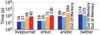
(a) REACH

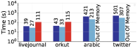
(b) CC

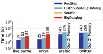
(c) SSSP

Figure 13: Performance Comparison on Real-World Graphs.

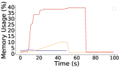
(a) REACH

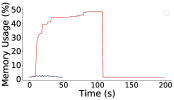
(b) CC

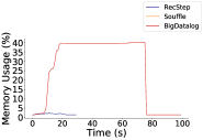
(c) SSSP

Figure 14: Memory Consumption on livejournal.

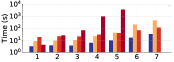
(a) AA on 7 synthetic datasets

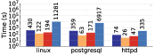
(b) CSDA on systems programs

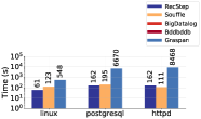
(c) CSPA on systems programs

Figure 15: Performance Comparison on Program Analyses

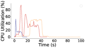
(a) AA on dataset 5

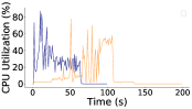
(b) CSPA on linux

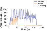
(c) CSPA on httpd

Figure 16: CPU Utilization on Program Analyses

Experiments of Other Graph Analytics Besides TC and SG, we also perform experiments running REACH, CC and SSSP on both the RMAT graphs and the real world graphs (Table 3), comparing the execution time and memory consumption (on livejournal) of our system with Souffle and BigDatalog (Figure 13, 14) . Since Soufflle does not support recursive aggregation (which shows in CC and SSSP), we only show the execution time results of our system and BigDatalog for CC and SSSP. bddbddb is excluded, since the number of vertices of all the graphs is too large.

As mentioned in [23], the size of the intermediate results produced during the evaluation of REACH, CC, SSSP is $O(m)$, $O(dm)$ and $O(nm)$, where $n$ is the number of vertices, $m$ is the number of edges and $d$ is the diameter of the graph. For convenience of comparison, we follow the way in which [23] presents the experiments results: for REACH and SSSP, we report the average run time over ten randomly selected vertices. We only consider an evaluation complete if the system is able to finish the evaluation on all ten vertices for REACH and SSSP, otherwise, the evaluation is seen as failed (due to OOM). The corresponding point of failed evaluation is not reported in Figure 12 (on RMAT graphs) and is shown as Out of Memory in Figure 13 (on real world graphs).

Besides Distributed-BigDatalog, RecStep is the only system that completes the evaluation for REACH, CC, SSSP on all RMAT graphs and real world graphs, and is 3-6X faster than other systems using scale-up approach on all the workloads that other systems manage to finish (as shown in Figures 12 and 13); compared to Distributed-BigDatalog, RecStep shows comparable performance using far less computational resource. Both BigDatalog and Souffle fail to finish evaluating some of the workloads due to OOM. As shown in Figure 12, the execution time of our system increases nearly proportionally to the increasing size of the dataset on all three graph analytics tasks. In contrast, Souffle’s parallel behavior is workload dependent though it efficiently evaluates dataflow and points-to analysis (Fig 15(b), 15(c)), it does not fully utilize all the CPU cores when evaluating REACH (Fig13(a), 12(a)) and Andersen’s analysis (Fig 15(a) ) .The CPU utilization of different system evaluating Andersen’s analysis, CSPA is visualized in Figure 16.

Program Analysis. We perform experiments on Andersen’s analysis using the synthetic datasets (generated based on a real-world dataset). Besides, we also conduct experiments comparing the execution time of CSPA and CSDA on the real system programs in [25]. Nonlinear recursive rules are commonly observed in Datalog programs for program analysis, and the results help us understand the behavior of our system and other systems when evaluating Datalog programs involving/without involving complex recursive rules.

For Andersen analysis, the number of variables (the size of active domains of each edb relation) increases from dataset 1 to dataset 7. Our system outperforms all other systems on every dataset. The performance of bddbddb is comparable to other systems when the number of variables being considered is small (dataset 1 and dataset 2), but the runtime increases a lot when the number of variables grows, due to its large overhead of building the bdd. BigDatalog outperforms Souffle on large datasets, since Souffle does not parallelize the computation as effectively.

All three systems significantly outperform Graspan on both CSPA and CSDA, as shown in Figure 15(b) and Figure 15(c). Since BigDatalog does not support mutual recursion, it is not present in Figure 15(c)). The inefficiency of Graspan is mainly due to its frequent use of sorting, coordination during the computation and relatively poor utilization of multi-cores for parallel computation.

CSDA is the only Datalog program on which RecStep is outperformed by Souffle and BigDatalog and the reasons are two-fold. First, the evaluation of CSDA on all three datasets needs many iterations ($\sim 1000$), and thus the overhead of triggering each query including compiling the query plan accumulates. There is also an additional overhead from the analyze calls and the materialization cost of the intermediate results. Compared to this overhead, the cost of the actual computation is much smaller. The second reason is that the rules in CSDA are simple and linear. Since the input data and the intermediate results produced in each iteration is small in size, the RDBMS cannot fully utilize the available cores.

In contrast, CSPA has more rules and involves nonlinear recursion, producing large $\Delta$ and intermediate results at each iteration. This enables RecStep to exploit both data-level and multiquery-level parallelism. Figure 15(c) shows the evaluation time for CSPA: while Souffle slightly outperforms our system on the httpd dataset, RecStep outperforms Souffle and Graspan on the other two datasets.

7 Conclusion

In this paper, we presented the design and implementation of RecStep, a general-purpose, parallel, in-memory Datalog solver, along with the experimental comparison results of existing techniques. Specifically, we demonstrated how to implement an efficient, parallel Datalog solver atop a relational database. To achieve high efficiency, we presented a series of algorithms, data structures, and optimizations, at the level of Datalog compilation to sql and at the level of the underlying rdbms. Our results demonstrate the scalability of our approach, its applicability to a range of application domains, and its competitiveness with highly optimized and specialized Datalog solvers. The experimental evaluation helps revealing the advantages and disadvantages of the existing techniques and guides the design and implementation of RecStep.

Appendix A Cost Model of DSD

Algorithm 4 One-Phase Set-Difference (OPSD)

1:Input: $R,R_{\delta}$

2:Output: $\Delta{R}\leftarrow R_{\delta}-R$

3:$HS\leftarrow\mathsf{buildHashTable}(R)$

4:$\Delta R\leftarrow\mathsf{antiJoinProbe}(R_{\delta},HS)$

Algorithm 5 Two-Phase Set-Difference (TPSD)

1:Input: $R,R_{\delta}$

2:Output: $\Delta{R}\leftarrow R_{\delta}-R$

3:$B\leftarrow$ smallest of $R_{\delta},R$

4:$P\leftarrow$ largest of $R_{\delta},R$

5:$HB\leftarrow\mathsf{buildHashTable}(B)$

6:$r\leftarrow\mathsf{joinProbe}(P,HB)$ $\triangleright$ $r\leftarrow B\Join P$

7:$Hr\leftarrow\mathsf{buildHashTable}(r)$

8:$\Delta R\leftarrow\mathsf{antiJoinProbe}(R,Hr)$ $\triangleright$ $\Delta{R}\leftarrow R_{\delta}-r$

The cost of OPSD and TPSD:
(1)

$$Cost (OPSD)=$$

$$C_{b}\cdot|R|+C_{p}\cdot|R_{\delta}|$$

$$Cost (TPSD)=$$

$$C_{b}\cdot(min(|R|,|R_{\delta}|)+|r|)+C_{p}\cdot(max(|R|,|R_{\delta}|)+|R_{\delta}|)$$

Furthermore, the difference between the cost of OPSD and cost of TPSD is:
(2)

$$Cost(OPSD)-Cost(TPSD)=$$

$$C_{b}\cdot|R|-C_{b}\cdot min(|R|,|R_{\delta}|)-C_{b}\cdot|r|-C_{p}\cdot max(|R|,|R_{\delta}|)$$

We can see from the cost model that the selection between the two set-difference algorithms depends on the sizes of $S$ and $R$ (in every iteration) and thus we discuss the two cases separately as follows:
If $|R|\leq|R_{\delta}|$:
(3)

$$Cost(OPSD)-Cost(TPSD)=-(C_{b}\cdot|r|+C_{p}\cdot|R_{\delta}|)<0$$

If $|R|>|R_{\delta}|$:
(4)

$$Cost(OPSD)-Cost (TPSD)=$$

$$(C_{b}-C_{p})\cdot|R|-C_{b}\cdot(|R_{\delta}|+|r|)$$

We can see that the selection between OPSD and TPSD for set-difference is not clear based on the above formulation when $|R|>|R_{\delta}|$, thus we use additional parameters to help with the analysis. Denoting $C_{b}=\alpha C_{p}$, $|R|=\beta|R_{\delta}|$ and $|R_{\delta}|=\mu|r|$, where $\alpha,\beta,\mu\in\mathbb{R^{+}}$. Then we can rewrite the cost difference between OPSD and TPSD (when $|R|>|R_{\delta}|$) as:
(5)

$$Cost(OPSD)-Cost (TPSD)=$$

$$\mu\cdot|r|\cdot C_{p}\cdot[\beta(\alpha-1)-(\alpha+\frac{\alpha}{\mu})]$$

While we can know the accurate value of $\beta$ and $\alpha$, there is no way to know the accurate value of $\mu$ beforehand (before selecting between OPSD and TPSD). However, we do know that $|r|\leq|R_{\delta}|$ and thus $\mu\geq 1$ (when $|r|=0$, the cost difference can be easily calculated from (4)) . Using this information, we can further derive the lower bound of the cost difference:
(6)

$$\mu\cdot|r|\cdot C_{p}\cdot[\beta(\alpha-1)-(\alpha+\frac{\alpha}{\mu})]$$

$$\geq\mu\cdot|r|\cdot C_{p}\cdot[\beta(\alpha-1)-2\alpha]$$

Thus if $\beta\geq\frac{2\alpha}{\alpha-1}$, then $Cost(OPSD)-Cost(TPSD)>0$ and TPSD is used for set-difference computation. In a word, there is a clear guide for the selection of two set-difference algorithm when $\beta\in(0,1]\cup[\frac{2\alpha}{\alpha-1},+\infty]$. Though when $\beta$ lies in $(1,\frac{2\alpha}{\alpha-1})$, the cost difference between two set-difference algorithm is not certain, we observe that in many of the workloads, the value difference of $\mu$ in two consecutive iterations is small, and thus a heuristic approach for choosing between OPSD and TPSD when $\beta$ lies in $(1,\frac{2\alpha}{\alpha-1})$ is to use the value of $\mu$ in previous iteration to approximate the value of $\mu$ in the current iteration. The value of $\alpha$ is pre-computed from offline training: perform $k$ join runs on $n$ table pairs $\{\langle S_{i},R_{i}\rangle$ $|$ $i=1,2,...n\}$ of different sizes (ensure $|R_{i}|\leq|S_{i}|$, suggesting the hash table is always built on $R_{i}$). In $j$ join run on $\langle S_{i},R_{i}\rangle$, denote the build cost as ${{B_{i}}_{j}}$ and the probe cost as ${{P_{i}}_{j}}$, then:
(7)

$$\alpha=\sum_{i}^{n}{\frac{\sum_{j}^{k}{\frac{{B_{i}}_{j}\cdot|R_{i}|}{{P_{i}}_{j}\cdot|S_{i}|}}}{k}}$$

The values of $k,n$ and table pairs $\{\langle S_{i},R_{i}\rangle|i=1,2,...n\}$ are pre-specified.

Appendix B CPU Efficiency

The CPU efficiency is workload dependent. A workload ($w$) is defined as a combination of a specific dataset ($d$) and a specific program ($p$). The runtime of a certain system ($s$) on a workload $w$ consisting of $d$ and $p$ is denoted as $t^{s}_{w(p,d)}$. Denoting the number of CPU cores given for $s$ (which supports multi-core computation) as $n$, the CPU efficiency ($ce$) is defined as $ce=\frac{1}{t^{s}_{w(p,d)}\cdot n}$. Intuitively, if $s$ can efficiently utilize CPU given multiple-cores, the value of $t^{s}_{w(p,d)}\cdot n$ should be relatively small and $ce$ should be relatively large. Table 4 presents the CPU efficiency of different systems on multiple chosen representative workloads.

	Graspan	BigDatalog	Distributed-BigDatalog	Souffle	RecStep
TC (G20K)	-	2.75e-04	4.39e-04	2.92e-04	1.12e-03
SG (G10K))	-	7.18e-05	3.47e-04	5.41e-04	2.45e-03
REACH (orkut)	-	1.92e-04	4.17e-04	3.52e-04	1.32e-03
CC (orkut)	-	2.17e-04	2.53e-04	-	5.81e-04
SSSP (orkut)	-	1.81e-04	2.14e-04	-	1.00e-03
AA (dataset 7)	-	2.20e-04	-	5.65e-05	7.65e-04
CSDA (linux)	2.22e-06	1.29e-04	-	2.05e-04	5.81e-05
CSPA (linux)	4.56e-05	-	-	2.03e-04	4.10e-04

Table 4: CPU Efficiency of Different Systems

Appendix C Time and Space Effect Analysis of Optimizations

Besides the empirical study of the time and memory effect of each optimization technique shown in Figure 2 and Figure 3, we discuss here about the time and space effect of each optimization in more detail.

1. Unified idb Evaluation (uie): different rules and different subqueries inside each recursive rule evaluating the same idb relation are issued as a single query without introducing explicit coordination overhead for multiple concurrent running subqueries while enabling better parallelism and pipelining. For in-memory evaluation, uie enables to share the hash-table(s) built on the same table(s), thus merely increases the peak memory consumption (edb tables and idb tables from previous iterations already reside in memory).

2. Optimization On the Fly (oof): lightweight analytical queries are executed on data that is already in memory at specified breakpoint to collect necessary statistical data, which adds small runtime overheads without influencing the peak memory usage. The technique can result in great performance boost by making the relatively-long running query run right after the breakpoint choose the correct query plan. However, if there are too many after-breakpoint queries that are too short (shorter than the analytical queries, which is unlikely to happen frequently), then oof will slow down the whole evaluation performance.

3. Dynamic Set Difference (dsd): the technique guides the choice of the set-difference algorithm that takes less time and adds negligible computational overheads from cost-model computation, which is barely a few mathematical operations. By exploiting the cost-model for DSD, table of smaller size is chosen to build the hash table on and thus the memory consumption is minimized.

4. Evaluation as One Single Transaction (eost): for in-memory evaluation, when memory is big enough for all the data to fit into, delaying the dirty pages produced during any of the intermediate operations until the end of evaluation avoids non-necessary I/O cost and has no influence on the memory usage.

5. Fast Deduplication (fast-dedup): the technique speed-ups the Datalog program evaluation by reducing the cost of hashing (using tuple itself as hash value) and chance of collision compared to the original parallel global separate chaining hash table. It achieves memory saving by eliminating the use of extra hash key and pointer to the tuple when the number of attributes of the tuple is small. fast-dedup can possibly increase the peak memory usage during the deduplication phase if the number of attributes of the tuples in the table to be deduplicated is large (when the memory consumed by the compact key is larger than the memory needed by the hash key and pointer).

References

- [1] S. Abiteboul, R. Hull, and V. Vianu, editors. Foundations of Databases: The Logical Level. Addison-Wesley Longman Publishing Co., Inc., Boston, MA, USA, 1st edition, 1995.
- [2] F. N. Afrati, V. R. Borkar, M. J. Carey, N. Polyzotis, and J. D. Ullman. Map-reduce extensions and recursive queries. In EDBT ’11, pages 1–8, 2011.
- [3] F. N. Afrati and J. D. Ullman. Transitive closure and recursive datalog implemented on clusters. In EDBT ’12, pages 132–143, 2012.
- [4] L. O. Andersen. Program analysis and specialization for the C programming language. PhD thesis, University of Cophenhagen, 1994.
- [5] T. Antoniadis, K. Triantafyllou, and Y. Smaragdakis. Porting doop to soufflé: a tale of inter-engine portability for datalog-based analyses. In Proceedings of the 6th ACM SIGPLAN International Workshop on State Of the Art in Program Analysis, pages 25–30. ACM, 2017.
- [6] https://www.cloudlab.us/, 2018.
- [7] R. Fagin, P. G. Kolaitis, R. J. Miller, and L. Popa. Data exchange: Semantics and query answering. In Database Theory - ICDT 2003, 9th International Conference, Siena, Italy, January 8-10, 2003, Proceedings, pages 207–224, 2003.
- [8] T. J. Green, M. Aref, and G. Karvounarakis. Logicblox, platform and language: A tutorial. In Datalog in Academia and Industry, pages 1–8. Springer, 2012.
- [9] D. Halperin, V. T. de Almeida, L. L. Choo, S. Chu, P. Koutris, D. Moritz, J. Ortiz, V. Ruamviboonsuk, J. Wang, A. Whitaker, S. Xu, M. Balazinska, B. Howe, and D. Suciu. Demonstration of the myria big data management service. In SIGMOD ’14, pages 881–884, 2014.
- [10] M. Han and K. Daudjee. Giraph unchained: barrierless asynchronous parallel execution in pregel-like graph processing systems. Proceedings of the VLDB Endowment, 8(9):950–961, 2015.
- [11] H. Jordan, B. Scholz, and P. Subotić. Soufflé: On synthesis of program analyzers. In International Conference on Computer Aided Verification, pages 422–430. Springer, 2016.
- [12] A. Lefebvre. Towards an efficient evaluation of recursive aggregates in deductive databases. In FGCS, pages 915–925, 1992.
- [13] M. Lenzerini. Data integration: A theoretical perspective. In Proceedings of the Twenty-first ACM SIGACT-SIGMOD-SIGART Symposium on Principles of Database Systems, June 3-5, Madison, Wisconsin, USA, pages 233–246, 2002.
- [14] B. T. Loo, T. Condie, M. N. Garofalakis, D. E. Gay, J. M. Hellerstein, P. Maniatis, R. Ramakrishnan, T. Roscoe, and I. Stoica. Declarative networking: language, execution and optimization. In Proceedings of the ACM SIGMOD International Conference on Management of Data, Chicago, Illinois, USA, June 27-29, 2006, pages 97–108, 2006.
- [15] G. Malewicz, M. H. Austern, A. J. Bik, J. C. Dehnert, I. Horn, N. Leiser, and G. Czajkowski. Pregel: a system for large-scale graph processing. In Proceedings of the 2010 ACM SIGMOD International Conference on Management of data, pages 135–146. ACM, 2010.
- [16] B. Motik, Y. Nenov, R. Piro, I. Horrocks, and D. Olteanu. Parallel materialisation of datalog programs in centralised, main-memory RDF systems. In AAAI ’14, pages 129–137, 2014.
- [17] J. M. Patel, H. Deshmukh, J. Zhu, N. Potti, Z. Zhang, M. Spehlmann, H. Memisoglu, and S. Saurabh. Quickstep: A data platform based on the scaling-up approach. PVLDB, 11(6):663–676, 2018.
- [18] T. W. Reps. Program analysis via graph reachability. In J. Maluszynski, editor, ILPS, pages 5–19. MIT Press, 1997.
- [19] B. Scholz, H. Jordan, P. Subotić, and T. Westmann. On fast large-scale program analysis in datalog. In Proceedings of the 25th International Conference on Compiler Construction, CC 2016, pages 196–206, New York, NY, USA, 2016. ACM.
- [20] J. Seo, S. Guo, and M. S. Lam. Socialite: Datalog extensions for efficient social network analysis. In 29th IEEE International Conference on Data Engineering, ICDE 2013, Brisbane, Australia, April 8-12, 2013, pages 278–289, 2013.
- [21] J. Seo, J. Park, J. Shin, and M. S. Lam. Distributed socialite: A datalog-based language for large-scale graph analysis. PVLDB, 6(14):1906–1917, 2013.
- [22] M. Shaw, P. Koutris, B. Howe, and D. Suciu. Optimizing large-scale semi-naïve datalog evaluation in hadoop. In Datalog 2.0, pages 165–176, 2012.
- [23] A. Shkapsky, M. Yang, M. Interlandi, H. Chiu, T. Condie, and C. Zaniolo. Big data analytics with datalog queries on spark. In SIGMOD ’16, pages 1135–1149, 2016.
- [24] J. Wang, M. Balazinska, and D. Halperin. Asynchronous and fault-tolerant recursive datalog evaluation in shared-nothing engines. PVLDB, 8(12):1542–1553, 2015.
- [25] K. Wang, A. Hussain, Z. Zuo, G. Xu, and A. Amiri Sani. Graspan: A single-machine disk-based graph system for interprocedural static analyses of large-scale systems code. In Proceedings of the Twenty-Second International Conference on Architectural Support for Programming Languages and Operating Systems, ASPLOS ’17, pages 389–404, New York, NY, USA, 2017. ACM.
- [26] J. Whaley, D. Avots, M. Carbin, and M. S. Lam. Using datalog with binary decision diagrams for program analysis. In Proceedings of the Third Asian Conference on Programming Languages and Systems, APLAS’05, pages 97–118, Berlin, Heidelberg, 2005. Springer-Verlag.
- [27] J. Whaley and M. S. Lam. Cloning-based context-sensitive pointer alias analysis using binary decision diagrams. In W. Pugh and C. Chambers, editors, PLDI, pages 131–144. ACM, 2004.
- [28] C. Zaniolo, M. Yang, M. Interlandi, A. Das, A. Shkapsky, and T. Condie. Declarative bigdata algorithms via aggregates and relational database dependencies. In Proceedings of the 12th Alberto Mendelzon International Workshop on Foundations of Data Management, Cali, Colombia, May 21-25, 2018., 2018.