Abstract

The simulation of thermochemical nonequilibrium for the atomic and molecular energy level populations in plasma flows requires a comprehensive modeling of all the elementary collisional and radiative processes involved. Coupling detailed chemical mechanisms to flow solvers is computationally expensive and often limits their application to 1D simulations. We develop an efficient Lagrangian diffusive reactor moving along the streamlines of a baseline flow simulation to compute detailed thermochemical effects. In addition to its efficiency, the method allows us to model both continuum and rarefied flows, while including mass and energy diffusion. The Lagrangian solver is assessed for several testcases including strong normal shockwaves, as well as 2D and axisymmetric blunt-body hypersonic rarefied flows. In all the testcases performed, the Lagrangian reactor improves drastically the baseline simulations. The computational cost of a Lagrangian recomputation is typically orders of magnitude smaller with respect to a full solution of the problem. The solver has the additional benefit of being immune from statistical noise, which strongly affects the accuracy of DSMC simulations, especially considering minor species in the mixture. The results demonstrate that the method enables applying detailed mechanisms to multidimensional solvers to study thermo-chemical nonequilibrium flows.

1 Introduction

A broad range of high-enthalpy and plasma technology applications exhibit thermochemical nonequilibrium effects, for instance in the fields of thermal plasmas,[1] combustion, [2] plasma-assisted ignition,[3, 4] diagnostics,[5, 6] solar physics,[7, 8] laser ablation, [9] surface coating, [10] and in general, materials technology.[11] In aerospace applications, the radiative heat flux to the heat shield of planetary entry probes [12, 13] depends on the populations of atomic and molecular internal energy levels, often out of equilibrium. In particular, many chemically reacting species are present in atmospheric entry flows for space vehicles reaching entry velocities higher than 10 km/s.[14, 15] With the ambition of deep space exploration, detailed chemical mechanisms become of primary importance to optimize the efficiency of electric propulsion thrusters.[16, 17]

The simulation of thermochemical nonequilibrium for the atomic and molecular energy level populations in plasma flows requires a comprehensive modeling of all the elementary collisional and radiative processes involved. Detailed simulations are based on a large set of chemical species and their related chemical mechanism.[18, 19, 20, 21, 22, 23] Coupling such mechanisms to flow solvers is computationally expensive and often limits their application to 1D simulations. Moreover, since the timescales of the physico-chemical phenomena vary widely, the discretization of the convective and diffusive fluxes, as well as chemical production rates, necessitates a specific numerical treatment.[24, 25, 26]

The simulation of non-trivial geometries becomes feasible by adopting strategies to lower the computational cost associated with chemistry modeling, while retaining a good level of physical realm; principal component analysis (PCA),[27] energy levels binning,[23, 28] and rate-controlled constrained-equilibrium (RCCE)[29] being some possible approaches. Yet, the problem remains complicated enough to run out of the current supercomputing capabilities when real-world applications or design loops are targeted. A pragmatic way to address the problem still consists in making strong simplifying assumptions.

In the chemistry and combustion communities, the idea of decoupling flow and chemistry is used to include detailed thermochemical effects into lower-fidelity baseline solutions, [30] and also to formulate hybrid Eulerian-Lagrangian reactors.[31] In atmospheric entry plasmas, a Lagrangian method using a collisional-radiative reactor has been coupled to a flow solver, [32] based on the 1D method proposed by Thivet to study the relaxation of chemistry past a shockwave.[33] Lagrangian tools, allowing for the refinement of an existing solution with very small computational effort, are based on fluid models.

Fluid models for plasma flows can be derived from kinetic theory as asymptotic solutions to the Boltzmann equation, provided that the Knudsen number is small enough.[34, 35, 36] For instance, Graille $et~{}al.$ [37] have obtained a perturbative solution for multicomponent plasmas based on a multiscale Chapmann-Enskog method by accounting for the disparity of mass between the electrons and heavy particles, as well as for the influence of the electromagnetic field. When the Knudsen number is too large to be in the continuum regime, the Maxwell transfer equations can be derived by directly averaging microscopic properties in the velocity space and by using the collisional operator properties.[38] This set of balance equations for mass, momentum, and total energy holds in both the continuum and rarefied regimes. The difficulty is then to find a closure for the transport fluxes appearing in the Maxwell transfer equations. A direct numerical simulation of the kinetic equations can be used to compute these fluxes.[39]

The aim of this work is to develop a method for including detailed thermochemical effects into lower-fidelity baseline solutions through an efficient Lagrangian diffusive reactor. Our approach starts from a baseline solution for a plasma flow, by extracting the velocity and total density fields along its streamlines, and thus decoupling thermochemical effects from the flowfield. The main assumption is that fine details of the species energy level populations, as well as trace species in the mixture, do not severely impact the hydrodynamic features of the flow. This is the case for many applications, such as the aerodynamics of a jet, the location of a detached shock wave, or the trail behind a body flying at hypersonic speed. As long as the total energy transfer can be modeled by means of some effective chemical mechanism, a more detailed description of the thermo-chemical state of the plasma can be obtained by re-processing the baseline calculation using more species and chemical reactions. The originality of this contribution consists in leveraging the Lagrangian nature of the proposed method, developing a general solution procedure based on an upwinded marching approach, adding rarefied, multi-dimensional, and dissipative effects. The consequence is a drastic boost in the computational efficiency, allowing to deal with a large number of chemical species.

We propose to develop a tool to obtain reasonably accurate predictions of the thermochemical state of a flow using an enlarged set of species and describing thermal nonequilibrium via multi-temperature, state-to-state, or collisional-radiative models. As a proof of concept, we account for radiation-flow coupling via escape factors. Reaching higher accuracies using detailed chemistry output of the Lagrangian reactor to solve the radiative transfer equation is beyond the scope of this work. The presented strategy can be employed as a design tool to obtain information too expensive for a fully coupled approach. Alternatively, it can also be used for diagnostic purposes to promptly estimate the effect of different physico-chemical models into realistic simulations: this allows us to understand whether a simplified modeling can be suitable for the considered problem. Finally, with respect to particle-based flow simulations, such as those obtained with the Direct Simulation Monte Carlo Method (DSMC),[39] the proposed method smooth out the noise and irregularities associated to the inherent stochastic approach, improving the prediction of minor species. Electronic energy levels, which would require a particularly detailed and computationally intensive approach otherwise,[40] can also be easily computed. The capabilities of the method are assessed against five problems, namely: (i) Chemical refinement, (ii) Thermal refinement, (iii) State-to-state refinement, (iv) 2D rarefied flow, and (v) Mass and energy diffusion. In all the performed testcases, we investigate the accuracy of the thermochemical description and its computational cost.

Section 2 of this work introduces the Lagrangian approach in terms of governing equations, physical modeling of fluxes and numerical implementation. The method is applied to the five testcases in section 3. Finally, in section 4 some conclusions and future perspectives on the tool developed are drawn.

2 Lagrangian reactor approach

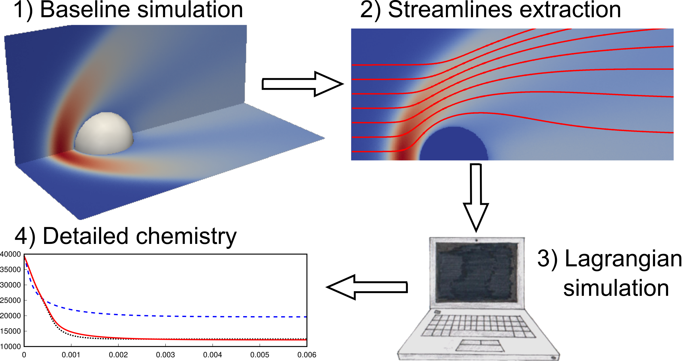
Figure 1: Procedure for applying the Lagrangian diffusive reactor to perform detailed thermochemical flow computations.

In this work, the flow is assumed to be steady, such that the trajectory of a fluid element coincides with its streamline. We propose to use this property in the development of a diffusive Lagrangian reactor moving along the streamlines. The solution procedure, sketched in Fig. 1, is as follows: (i) A baseline flow simulation is obtained using an effective thermo-chemical model; (ii) A suitable number of streamlines is extracted from the solution; (iii) The Lagrangian tool imports the baseline streamlines and recomputes the species mass and energy transfer using more chemical species and thermo-chemical processes. This variable volume chemical reactor follows a precomputed fluid element, and in the most elaborated approach developed, energy and mass are exchanged by diffusion with its neighbors over the computational domain. The velocity field is not recomputed but taken from the baseline simulation. The global mixture density comes directly from imposing a velocity field and is thus directly imported from the baseline simulation as well. Initial conditions for the species concentration and temperatures are picked at the beginning of the streamlines, and the new thermo-chemical state is calculated by integration of species mass conservation equations and suitable energy equations given in this section. It should be noted that there is no need for solving the momentum and global mass equations, since the velocity and density are imported. These fields introduce information about the flow topology, as well as its kinetic energy.

2.1 Maxwell transfer equations and nonequilibrium models

For quasi-neutral plasmas and in the absence of applied electro-magnetic field, the Maxwell transfer equations are expressed as follows[41, 42]

$$\frac{\partial}{\partial t}\begin{pmatrix}\rho_{i}\\ \rho\bm{u}\\ \rho E\end{pmatrix}+\bm{\nabla}\!\cdot\!\begin{pmatrix}\rho_{i}\bm{u}\\ \rho\bm{u}\bm{u}\\ \rho\bm{u}H\end{pmatrix}+\bm{\nabla}\!\cdot\!\begin{pmatrix}\rho_{i}\bm{V}_{i}\\ P\mathbb{I}+\bm{\tau}\\ \bm{\tau}\!\cdot\!\bm{u}+\bm{q}\end{pmatrix}=\begin{pmatrix}\omega_{i}\\ 0\\ \mathscr{P}\end{pmatrix},$$ (1)

where index $i\in\mathcal{S}$ spans the chemical species. The species partial density is introduced as $\rho_{i}$, together with the mixture density $\rho=\sum_{i\in\mathcal{S}}\rho_{i}$, hydrodynamic velocity $\bm{u}$, total energy $E$, and total enthalpy $H$. The transport fluxes are obtained as average fluxes of microscopic properties in the velocity space weighted by the species velocity distribution function $f_{i}$, which is solution to the Boltzmann equation that can be computed, for instance, by means of a stochastic particle method.[39] The species diffusion velocities are then expressed as an average mass flux, $e.g.$, $\bm{V}_{i}=\int_{\mathbb{R}^{3}}f_{i}m_{i}(\bm{c}_{i}-\bm{u})~{}\mathrm{d}\bm{c}_{i}$, for point particles $i\in\mathcal{S}$ without internal energy. In this contribution, the pressure tensor is assumed to be isotropic, quantity $P$ being the scalar mixture pressure and $\mathbb{I}$ the identity matrix; the reactive pressure is assumed to be negligible. Suitable expressions for the mixture viscous stress tensor $\bm{\tau}$ and heat flux $\bm{q}$ can be found in references.[43, 38] The $i$-species chemical production rates $\omega_{i}$ are given by the law of mass action recalled in appendix. [36, 44] Quantity $\mathscr{P}$ is the radiative power of the plasma considered as a participating medium. When the Knudsen number is small enough to use the Chapman-Enskog method, the transport fluxes are shown to be linearly proportional to transport forces. For instance, neglecting thermal diffusion, the diffusion velocities are modeled by means of the generalized Fick law, $\bm{V}_{i}=-\sum_{j\in\mathcal{S}}D_{ij}~{}\bm{d}_{j}$, $i\in\mathcal{S}$. The diffusion force is $\bm{d}_{i}=(\bm{\nabla}P_{i}-n_{i}q_{i}\bm{E})/P$, with the partial pressure $P_{i}$, number density $n_{i}$, and charge $q_{i}$ of species $i\in\mathcal{S}$, and the electric field $\bm{E}$.[45] In this case, the calculation of the species velocity distribution function is no longer required, since the multicomponent diffusion coefficients $D_{ij}$, $i,j\in\mathcal{S}$, have a closed form in terms of average cross-sections based on binary interaction potentials between the species pairs. [43]

Electrons and heavy particles can exhibit distinct temperatures due to their mass disparity. A balance equation for the free electrons energy can also be derived from the Boltzmann equation by using an average electron kinetic energy in the velocity space

$$\frac{\partial}{\partial t}(\rho_{e}e_{e}^{t})+\bm{\nabla}\!\cdot\!(\rho_{e}e_{e}^{t}\bm{u})+P_{e}\bm{\nabla}\!\cdot\bm{u}+\bm{\nabla}\!\cdot\bm{q}_{e}=\Omega_{e}+\mathscr{P}_{e},$$ (2)

where quantity $e_{e}^{t}$ is the translational energy of free electrons, $\bm{q}_{e}$, the electron heat flux, and $\mathscr{P}_{e}$, the electron radiative power. The source term $\Omega_{e}$ describes the exchange of energy between the free electrons and heavy particles through elastic collisions, as well as through inelastic collisions driven by electrons. The latter correspond to chemical reactions ($e.g.$ electron-impact ionization) and elementary processes of excitation for the internal energy modes of atomic and molecular species ($e.g.$ electron-impact excitation). The set of equations (1)-(2) allows for a state-to-state description of the plasma, considering the internal energy levels as pseudo-species. For instance, Cambier and Kapper [46] have studied a mixture of species comprising the electronic energy levels of a partially ionized argon gas for shock-tube experiments.

Multi-temperature models assume that the populations of the internal energy levels of the atoms and molecules follow Maxwell-Boltzmann distributions. They require less basic data and computational resources than state-to-state models, but they can be inaccurate when nonequilibrium prevails. In this framework, atomic and molecular internal degrees of freedom (rotational, vibrational, and electronic energy levels) are grouped into several modes supposed to be thermal baths of energy $e^{m}$ at a distinct temperature.[44] For each mode $m\in\mathcal{M}$ considered, an energy equation is expressed as

$$\frac{\partial}{\partial t}\left(\rho e^{m}\right)+\bm{\nabla}\!\cdot\left(\rho e^{m}\bm{u}\right)+\bm{\nabla}\!\cdot\bm{q}^{m}=\Omega^{m}+\mathscr{P}^{m},$$ (3)

where $\mathcal{M}$ is the set of energy modes. The source term $\Omega^{m}$ describes the exchange of energy through chemical reactions and excitation of internal energy modes. Quantity $\mathscr{P}^{m}$ is the radiative power for mode $m$. Notice that eq. (2) has a structure similar to the one of eq. (3), except for the term corresponding to the work of the electron compression force $P_{e}\bm{\nabla}\!\cdot\bm{u}$. The electron translational energy will thus be treated formally as an internal mode, separately or part of a thermal bath, depending on the ansatz followed (the electrons pressure term will be added accordingly).

Finally, when all the energy levels are found to be in equilibrium with a single thermal bath, the problem is degenerate and fully described by the system  (1) for conservation of mass, momentum, and total energy. For instance, Bruno and Giovangigli [47] have studied the convergence of a two-temperature model towards a one-temperature model based on kinetic theory, focusing on the relaxation of internal temperature and the concept of volume viscosity.

2.2 Governing equations for the Lagrangian reactor

The hydrodynamic velocity $\bm{u}$ is assumed to be known from a baseline simulation. The mixture density $\rho$ comes directly from the mass conservation and is also carried along without being recomputed. We recall that the diffusive Lagrangian reactor uses a more complete mechanism than in the baseline simulation. The set of chemical species can differ, as well as the model chosen to describe the population of the translational and internal energy levels, so that the species mass conservation equations need to be solved again. The translational temperatures of electrons and heavy particles and the temperatures of the internal energy baths, in the case of multi-temperature models, are computed using the relevant energy equations. The equations of Section 2.1 are recast in Lagrangian form along the streamlines. Assuming steady state conditions, the directional derivative is transformed into the operator $\bm{u}\cdot\bm{\nabla}\equiv U\tfrac{\partial}{\partial s}$, where $s$ is the curvilinear abscissa along the streamline, and $U$, the module of the velocity vector. This system is expressed in the general form

$$\frac{\partial Q}{\partial s}+A\ \bm{\nabla}\!\cdot(B\ \bm{\nabla}Q)=f,$$ (4)

where the source term vector is $f=f(Q)$. The transport fluxes are written in terms of gradients of the variables $Q$, based on a transport coefficient matrix $B(Q)$. The matrix $A(Q)$ comes from the transformation from conservative variables to the vector $Q$.

In the first equation of system (1), the species densities $\rho_{i}$ are substituted with the mass fractions $Y_{i}=\rho_{i}/\rho$. Invoking global mass conservation, $i.e.$, $\bm{\nabla}\cdot(\rho\bm{u})=0$, the species continuity equations are obtained in Lagrangian form as follows[48]

$$\frac{\partial Y_{i}}{\partial s}+\frac{1}{\rho U}\bm{\nabla}\!\cdot(\rho_{i}\bm{V}_{i})={\mathscr{S}_{i}^{Y}}\ ,\quad i\in\mathcal{S},$$ (5)

with mass source terms $\mathscr{S}_{i}^{Y}=\omega_{i}/(\rho U)$. The remaining equations depend on the choice of thermo-chemical model selected. Using the third equation of system (1), a conservation equation for the total enthalpy is found

$$\frac{\partial H}{\partial s}+\frac{1}{\rho U}\bm{\nabla}\!\cdot(\bm{\tau}\!\cdot\!\bm{u}+\bm{q})=\mathscr{S}^{H},$$ (6)

with the total enthalpy source term $\mathscr{S}^{H}=\mathscr{P}/(\rho U)$.

In a state-to-state approach, eq. (5) is written for the electrons and each energy level of the atoms and molecules, considered as separate species $i\in\mathcal{H}$ in the mixture, where symbol $\mathcal{H}=\mathcal{S}\setminus\{e\}$ stands for this extended set of heavy particles. The total enthalpy (per unit mass) is thus split into five terms: $H=\tfrac{1}{2}U^{2}+\sum_{j\in\mathcal{H}}(Y_{j}e_{j}^{f}+Y_{j}h_{j}^{t})+Y_{e}e^{f}_{e}+Y_{e}h^{t}_{e},~{}i.e.$, (i) the flow kinetic energy; heavy particles contribute through (ii) their internal energy, where quantity $\smash{e_{i}^{f}}$ is the formation contribution to the enthalpy of energy level $i\in\mathcal{H}$, (iii) their translational enthalpy, where $h_{i}^{t}$ is the translational contribution assumed to be at temperature $T$; free electrons contribute through (iv) their formation energy $e^{f}_{e}$, and (v) their translational enthalpy $h^{t}_{e}$ evaluated at temperature $T_{e}$. A suitable Lagrangian form is derived from global mass conservation for the expression $P_{e}\bm{\nabla}\cdot\bm{u}=-UP_{e}\tfrac{\partial}{\partial s}\ln\rho$ in eq. (2), which can thus be computed along a streamline of the baseline solution. Hence, an equation for the free electron temperature $T_{e}$ is easily derived from eq. (2)

$$\frac{\partial T_{e}}{\partial s}+\frac{1}{\rho_{e}Uc_{v,e}}\left[\bm{\nabla}\!\cdot\bm{q}_{e}-e_{e}^{t}\bm{\nabla}\!\cdot(\rho_{e}\bm{V}_{e})\right]=\mathscr{S}^{T_{e}},$$ (7)

where the electron temperature source term is introduced as $\mathscr{S}^{T_{e}}=(\mathscr{P}_{e}+\Omega_{e}+UP_{e}\tfrac{\partial}{\partial s}\ln\rho-e_{e}^{t}\omega_{e})/(\rho_{e}Uc_{v,e})$ and the specific heat at constant volume for electrons as $c_{v,e}=\mathrm{de_{e}^{t}}/{\mathrm{d}T_{e}}$. Then, using eq. (6), one gets after some algebra an equation for the heavy-particle temperature

$$\frac{\partial T}{\partial s}+\frac{1}{\rho Uc_{p,h}^{t}}\left[\bm{\nabla}\!\cdot(\bm{\tau}\!\cdot\!\bm{u}+\bm{q}-\gamma_{e}\bm{q}_{e})\right.\\ -\sum_{j\in\mathcal{S}}(h_{j}^{t}+e_{j}^{f})\bm{\nabla}\!\cdot(\rho_{j}\bm{V}_{j})+\gamma_{e}e_{e}^{t}\bm{\nabla}\!\cdot(\rho_{e}\bm{V}_{e})]=\mathscr{S}^{T},$$ (8)

where the heavy-particle temperature source term is $\mathscr{S}^{T}=[\mathscr{P}-\gamma_{e}(\mathscr{P}_{e}+\Omega_{e}+UP_{e}\tfrac{\partial}{\partial s}\ln{\rho})-\tfrac{1}{3}\rho\frac{\mathrm{d}}{\mathrm{d}s}U^{3}-$ $\sum_{j\in\mathcal{S}}(h_{j}^{t}+e_{j}^{f})\omega_{j}+\gamma_{e}e_{e}^{t}\omega_{e}]/(\rho Uc_{p,h}^{t})$, with the electron specific heat ratio $\gamma_{e}=c_{p,e}/c_{v,e}$ and specific heat at constant pressure $c_{p,e}=\mathrm{d}h_{e}^{t}/{\mathrm{d}T_{e}}$. The translational contribution of the frozen mixture specific heat at constant pressure $c_{p,h}^{t}=\sum_{j\in\mathcal{H}}Y_{j}c_{p,j}^{t}$ is based on quantity $c_{p,i}^{t}={\mathrm{d}h_{i}^{t}}/{\mathrm{d}T}$ for species $i\in\mathcal{H}$. To summarize, in the state-to-state approach, one solves eqs. (5), (7), and (8). The vector of unknowns for system (4) is $Q$ $=$ $[(Y_{i})_{i\in\mathcal{S}},~{}T,~{}T_{e}]^{\rm T}\in\mathbb{R}^{n}$ where the dimension $n=N+2$, with the number of species $N={\rm card}(\mathcal{S})$.

In a multi-temperature approach, the internal energy of mode $m$ is introduced as $\sum_{j\in\mathcal{S}}Y_{j}e_{j}^{m}$, where quantity $e_{i}^{m}$ is the mode energy for species $i$ evaluated at temperature $T^{m}$. An equation for the mode temperature is derived from eq. (3)

$$\frac{\partial T^{m}}{\partial s}+\frac{1}{\rho c_{v}^{m}U}\left[\bm{\nabla}\!\cdot\bm{q}^{m}-\sum_{j\in\mathcal{S}}e_{j}^{m}\bm{\nabla}\!\cdot(\rho_{j}\bm{V}_{j})\right]=\mathscr{S}^{T^{m}},$$ (9)

where $m\in\mathcal{M}$. The source term for temperature is introduced as $\mathscr{S}^{T^{m}}=(\mathscr{P}^{m}+\Omega^{m}+\aleph_{e}^{m}UP_{e}\tfrac{\partial}{\partial s}\ln{\rho}-\sum_{j\in\mathcal{S}}e_{j}^{m}\omega_{j})/(\rho Uc_{v}^{m})$. Quantity $c_{v}^{m}=\sum_{j\in\mathcal{S}}Y_{j}c_{v,i}^{m},$ is the contribution of the frozen mixture specific heat at constant volume for mode $m$. Quantities $e_{i}^{m}$ and $c_{v,i}^{m}=\mathrm{d}e_{i}^{m}/{\mathrm{d}T^{m}}$ are respectively the energy and specific heat of mode $m$ for species $i\in\mathcal{S}$. When the translation of free electrons is also included in the mode, $i.e.$, $e^{m}_{e}=e^{t}_{e}$ with $T_{e}=T^{m}$, eqs. (2) and (3) need to be summed before recasting them in the Lagrangian form given by eq. (9). The last equation is also valid when the thermal bath describes only the free electron translation, leading to the same structure as the one of eq. (7). In both cases, quantity $-P_{e}\bm{\nabla}\!\cdot\bm{u}$ is added to the source term by means of symbol $\aleph_{e}^{m}=1$ if electrons translational energy belongs to pool $m$, otherwise zero. Then, using eq. (6), one gets an equation for the translational mode of heavy particles

$$\frac{\partial T}{\partial s}+\frac{1}{\rho Uc_{p,h}^{t}}[\bm{\nabla}\!\cdot(\bm{\tau}\!\cdot\!\bm{u}+\bm{q})-\bm{\nabla}\!\cdot\sum_{m\in\mathcal{M}}\gamma^{m}\bm{q}^{m}\\ -\sum_{j\in\mathcal{S}}h_{j}\bm{\nabla}\!\cdot(\rho_{j}\bm{V}_{j})+{\displaystyle\sum_{\scriptsize\begin{array}[]{c}m\in\mathcal{M}\\ j\in\mathcal{S}\end{array}}}\gamma^{m}e_{j}^{m}\bm{\nabla}\!\cdot(\rho_{j}\bm{V}_{j})]=\mathscr{S}^{T},$$ (10)

where the heavy-particle temperature source term is $\mathscr{S}^{T}=[\mathscr{P}-\sum_{m\in\mathcal{M}}\gamma^{m}(\mathscr{P}^{m}+\Omega^{m}+\aleph_{e}^{m}UP_{e}\tfrac{\partial}{\partial s}\ln{\rho})-$ $\tfrac{1}{3}\rho\frac{\mathrm{d}}{\mathrm{d}s}U^{3}-\sum_{j\in\mathcal{S}}h_{j}\omega_{j}+\sum_{j\in\mathcal{S},m\in\mathcal{M}}\gamma^{m}e_{j}^{m}\omega_{j}]/(\rho Uc_{p,h}^{t})$, with the species enthalpies $h_{i}=h_{i}^{t}+\sum_{m\in\mathcal{M}}h_{i}^{m}+e_{i}^{f}$, $i\in\mathcal{H}$, and $h_{e}=h_{e}^{t}+e_{e}^{f}$, the ratio of frozen specific heats $\gamma^{m}={c_{p}^{m}}/{c_{v}^{m}}$ for mode $m$ and its contribution to the frozen mixture specific heat at constant pressure $c_{p}^{m}=\sum_{j\in\mathcal{S}}Y_{j}c_{p,i}^{m}$. Quantity $c_{p,i}^{m}=\mathrm{d}h_{i}^{m}/{\mathrm{d}T^{m}}$ is the specific heat at constant pressure of mode $m$ for species $i\in\mathcal{S}$. Notice the equality $c_{p,i}^{m}=c_{v,i}^{m}$, for heavy particles $i\in\mathcal{H}$. When some of the atomic and molecular internal degrees of freedom are grouped with the translational mode of heavy particles at the same bath temperature $T$, the expressions for the translational contribution of the enthalpy $h_{i}^{t}$ and specific heat $c_{p,i}^{t}$, $i\in\mathcal{H}$, used in Eq. (10), need to be modified accordingly. In the multi-temperature approach, one solves eq. (5), one eq. (9) for every mode $m$ considered, and eq. (10). The vector of unknowns is $Q$ $=$ $[(Y_{i})_{i\in\mathcal{S}},~{}T,~{}(T^{m})_{m\in\mathcal{M}}]^{\rm T}\in\mathbb{R}^{n}$, where dimension $n=N+M+1$, with the number of modes $M={\rm card}(\mathcal{M})$.

Finally, thermal equilibrium is obtained as a degenerate case of the multi-temperature approach

$$\frac{\partial T}{\partial s}+\frac{1}{\rho Uc_{p}}[\bm{\nabla}\!\cdot(\bm{\tau}\!\cdot\!\bm{u}+\bm{q})-\sum_{j\in\mathcal{S}}h_{j}\bm{\nabla}\!\cdot(\rho_{j}\bm{V}_{j})]=\mathscr{S}^{T},$$ (11)

where the heavy-particle temperature source term is $\mathscr{S}^{T}=[\mathscr{P}-\tfrac{1}{3}\rho\frac{\mathrm{d}}{\mathrm{d}s}U^{3}-\sum_{j\in\mathcal{S}}h_{j}\omega_{j}]/(\rho Uc_{p})$, with the contribution to the frozen mixture specific heat at constant pressure $c_{p}=\sum_{j\in\mathcal{S}}Y_{j}c_{p,j}$. The species enthalpy $h_{i}$, and specific heat at constant pressure $c_{p,i}$, $i\in\mathcal{S}$, are functions of a single temperature $T$, gathering all the translational and internal modes of the species, as well as their formation enthalpy. In the thermal equilibrium approach, one solves eqs. (5) and (11). The vector of unknowns is $Q$ $=$ $[(Y_{i})_{i\in\mathcal{S}},~{}T]^{\rm T}\in\mathbb{R}^{n}$, where dimension $n=N+1$.

2.3 Solution of the Lagrangian equations

In system (4), the structure of the diffusion term is of elliptic nature, which in principle requires to solve all the points of the domain simultaneously. In this work, two formulations are investigated to drastically reduce the computational cost: a decoupled single-streamline mode and a coupled multi-streamline mode.

Decoupled single-streamline mode. In the absence of diffusive terms in eq. (4), the system of Lagrangian equations simplifies as follows, ${\mathrm{d}Q}/{\mathrm{d}s}=f$, with the vector of unknowns $Q=Q(s)\in\mathbb{R}^{n}$. It is a system of explicit ordinary differential equations of order one and dimension $n$. This structure is of great benefice from the computational point of view since it allows to retrieve the solution by marching along the streamlines. In this case, the values of $Q$ can be computed along one independent streamline starting from an initial value $Q|_{s=0}=Q_{0}$, while the streamline shape can develop in a 3D space. Integration is performed using either an adaptive Runge-Kutta 4-5 or implicit Rosenbrock 4 scheme, from the C++ Boost library.[49]

A major drawback of this approach is that the fluid element is assumed to be adiabatic. This assumption may be acceptable considering the magnitude of the transport fluxes in advection-dominated (high Péclet number) flows. However, across shock waves, near non-adiabatic walls and, more generally, in flows with strong shear and fluxes, this assumption breaks down; one needs a way to compute diffusion fluxes through the fluid element.

A possible remedy consists in importing the variations of total enthalpy directly from the baseline solution. The diffusive fluxes are extracted from eq. (6) as follows

$$\frac{1}{\rho U}\bm{\nabla}\!\cdot(\bm{\tau}\!\cdot\!\bm{u}+\bm{q})=\frac{{\mathscr{P}}^{*}}{\rho U}-\frac{\Delta H^{*}}{\Delta s}$$ (12)

where symbol ^∗ refers to the baseline solution. The fluxes employed with this approach are not self-consistent, since they are entirely taken from the baseline flow, and not obtained from the recomputed solution. This approach should thus be considered more as a useful engineering ploy, rather than a rigorous treatment. Although not self-consistent, it has an interesting consequence: extending the applicability range of the Lagrangian reactor towards conditions of significant rarefaction, despite its fluid formulation. In fact, as long as the baseline solution is obtained with a method compliant with the rarefied regime (such as the DSMC method), the Lagrangian reactor imports such fluxes without the need of imposing any preassigned model.

Coupled multi-streamline mode. The second approach analyzed in this work aims at describing flows that show a preferential direction of development, such as boundary layers, jets, and trails, where diffusion mainly acts transversely. Calling $x$ the preferential and $r$ the transverse direction (orthogonal to it), diffusion terms in eq. (4) become purely transverse

$$\frac{\partial Q}{\partial s}+A\frac{\partial}{\partial r}\left(B\frac{\partial Q}{\partial r}\right)=f,$$ (13)

with the vector $Q=Q(r,s)\in\mathbb{R}^{n}$. Additionally, the preferential direction $x$ is chosen as a common reference to all the streamlines. The material derivative is recast from the curvilinear abscissa $s$ to the direction $x$ by introducing the local slope $\alpha_{k}$, such that $\mathrm{d}x=\cos{\alpha_{k}}\,\mathrm{d}s_{k}$, $k\in\mathcal{K}$, where $\mathcal{K}$ is the set of indexes for the streamlines. In this way, their phase is not lost during the integration (due to streamlines having different velocities) and governing equations can be integrated simultaneously, evaluating transverse diffusion terms implicitly at the current integration step, using a second-order central discretization. The parabolic system (13), written for each streamline $k$, becomes

$$\frac{\partial Q}{\partial x}+\frac{A}{\cos{\alpha_{k}}}\frac{\partial}{\partial r}\left(B\frac{\partial Q}{\partial r}\right)=\frac{f}{\cos{\alpha_{k}}},$$ (14)

The $x$ integration is performed as for the decoupled single-streamline mode with adaptive Runge-Kutta 4-5 or implicit Rosenbrock 4 schemes. Diffusion terms are discretized using a finite volume 1D formulation, where the cells are centered along the streamlines. Diffusion fluxes and source terms are evaluated implicitly by the routine, at every integration step. The simulation starts by imposing initial conditions $Q|_{s=0}=Q_{0}$ at the beginning of the streamline. Transverse fluxes evaluation requires imposing boundary conditions on the first and last streamlines, which can be either of Dirichlet (thermodynamic state imposed) or Neumann (zero gradient) type. In axisymmetric configuration, fluxes are imposed by symmetry on the lowest cell interface, located at the axis ($r=0$).

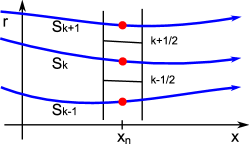
Figure 2: Streamline marching scheme with implicit transverse finite volume method.

The physico-chemical properties are obtained through the Open Source Mutation++ library.[50, 51]

The implementation of the coupled multi-streamline Lagrangian approach in a C++ language code has been verified by comparison of the analytical solution to a scalar diffusion equation ${\partial Q}/{\partial s}=\alpha~{}{\partial^{2}Q}/{\partial r^{2}}$, where quantity $\alpha$ is a nonnegative constant. The problem of diffusion in a semi-infinite domain can be shown to have a self-similar solution, the similarity variable being $r/\sqrt{4\alpha x}$, and its solution is given in terms of the Gauss error function.[52] Given a maximum value for the independent variable $x_{max}$, parallel streamlines were created at positions from $r=0$ up to $r=10\sqrt{4\alpha x_{max}}$, where fluxes are negligible. The thermodynamic state $Q$ was imposed on the bottom streamline and null fluxes (Neumann BC) on the top one. Using about 20 streamlines, with a progressively increasing spacing, allowed to retrieve the analytical solution within a few $\%$ accuracy. Increasing the number of streamlines reproduces the exact solution.

3 Results

In this section, the Lagrangian approach is assessed for five types of problems. The chemical (A) and thermal (B) refinement capabilities are tested in the continuum regime for the thermo-chemical relaxation of an air mixture past a strong 1D shockwave, using both single and multi-temperature models. The state-to-state refinement (C) is analyzed in the continuum regime for the excitation and ionization of an argon plasma past a strong 1D shockwave, then applied to the rarefied regime based on a 2D simulation using the DSMC method and accounting for radiative processes (D). Finally, mass and energy diffusion capabilities are tested in air for the rarefied regime along the trail past a blunt body moving at hypersonic speed (E).

3.1 Chemical refinement

We study the chemical relaxation in air past a strong 1D shockwave by assuming thermal equilibrium. Freestream conditions representative of the trajectory point at 1636 s of the Fire II flight experiment [53, 54] are given in Table 1.

$V_{\infty}$ [m/s]	$P_{\infty}$ [Pa]	$T_{\infty}$ [K]
11 310	5.25	210

Table 1: Freestream conditions for Fire II trajectory point at 1636 s (Testcases A and B).

Two mixtures are considered in this section: a neutral mixture composed of 5 species denoted by the set $\mathcal{S}_{5}=\{\mathrm{N_{2}}$, $\mathrm{O_{2}}$, $\mathrm{NO}$, $\mathrm{N}$, $\mathrm{O}\}$, so-called “air-5,” and a partially ionized mixture composed of 11 species denoted by the set $\mathcal{S}_{11}=\{\mathrm{N_{2}}$, $\mathrm{O_{2}}$, $\mathrm{NO}$, $\mathrm{N}$, $\mathrm{O}$, $\mathrm{N_{2}^{+}}$, $\mathrm{O_{2}^{+}}$, $\mathrm{NO^{+}}$, $\mathrm{N^{+}}$, $\mathrm{O^{+}}$, $\mathrm{e^{-}}\}$, so-called “air-11.” The chemical mechanism and rate coefficients are taken from Park $et~{}al.$ [55] The initial composition is assumed to be in local thermodynamic equilibrium at the freestream conditions. First, the post-shock mass, momentum, and total energy are computed using the Rankine-Hugoniot relations, keeping the chemical composition frozen. The baseline solution is obtained by solving numerically the system (1) for the air-5 mixture in steady conditions, following the approach proposed by Thivet.[33] The solution in the post-shock region is then recomputed by means of the Lagrangian reactor, which imports the velocity and density fields. The Lagrangian eqs. (15) and (17) presented in Appendix are solved using the air-11 mixture. Finally, the results of the Lagrangian simulation are compared to a reference solution to system (1) obtained for the air-11 mixture.

The temperature and species concentration along the stagnation line are shown in Figs. 3 and 4.

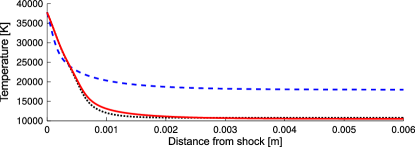
Figure 3: Chemical refinement for Fire II-Testcase A: temperature in the post-shock region; - - - baseline simulation (air-5); —– Lagrangian simulation (air-5 $\rightarrow$ air-11); $\bm{\cdots}$ reference simulation (air-11).

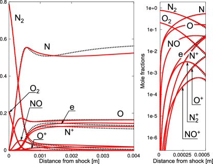
Figure 4: Chemical refinement for Fire II-Testcase A: species mole fractions in the post-shock region. Left: linear scale; right: logarithmic scale, detail of near-shock region; —– Lagrangian simulation (air-5 $\rightarrow$ air-11); $\bm{\cdots}$ reference simulation (air-11).

The Lagrangian simulation results eventually reach equilibrium values in agreement with the reference simulation. It is noteworthy that ions and free electrons, not present in the baseline solution, are reproduced with good accuracy. The discrepancies between the Lagrangian and reference results start around the position $x=5\times 10^{-4}\,\textrm{m}$, where the bulk of ionization occurs. In the reference computation, energy is spent to ionize the species; the kinetic energy is thus reduced. The error originates from the derivative of the kinetic energy flux $U^{3}$, appearing in eq. (17). However, the results are in fair agreement. Notice that the mass flux $\rho U$ is an invariant of all the simulations; this term, appearing at the denominator of the source term of the Lagrangian solution, does not introduce any approximation.

This testcase shows the chemical refinement capabilities of the method: the temperature field departs from the baseline solution shortly after the shock and, together with the chemical composition, closely follows the reference result. In general, the smaller the influence of the new chemical model on the baseline energy balance, the greater the expected accuracy. If only trace species are introduced, small degrees of ionization or dissociation almost do not alter the energy balance and the method retrieves the right solution with a very good degree of accuracy. However, this criterion is much less strict than it seems: in the simulation presented, newly-introduced ions reach concentrations over 10%, yet the solution is reproduced with reasonable accuracy.

3.2 Thermal refinement

We study the thermo-chemical relaxation in air past a strong 1D shockwave for the air-5 mixture, allowing for thermal nonequilibrium to occur. The translational energy of heavy particles and rotational energy of molecules are assumed to be in equilibrium at temperature $T$, while the vibrational energy of molecules and electronic energy of heavy particles are at temperature $T^{v}$. The freestream pressure and temperature are identical to the ones of Testcase A, while the velocity was reduced to $7000$ m/s to better comply with the air-5 model. With the same spirit as in the previous section, the solution is recomputed in the post-shock region by means of the Lagrangian reactor using a two-temperature ($T$-$T^{v}$) model, starting from a single-temperature baseline solution. The Lagrangian eqs. (15), (18), and (19) presented in Appendix are solved using the same air-5 mixture. A reference solution is obtained for the air-5 mixture by solving in steady conditions the system (1) coupled to eq. (3) for the mode at temperature $T^{v}$, following the approach proposed by Magin $et~{}al.$ [32]

The single-temperature post-shock conditions used for the baseline solution satisfy thermal equilibrium, whereas the two-temperature conditions used for the reference solution assume that the vibrational-electronic mode is frozen, so that the translational temperature $T$ jumps, while the internal temperature $T^{v}$ remains at its freestream value. The two temperatures then relax towards each other and eventually equilibrate at the same value reached by the single-temperature solution.

The Lagrangian solution takes the velocity and density fields from the single-temperature baseline computation, but starts with temperatures out of equilibrium. The solution is shown in Figs. 5 and 6.

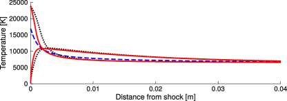
Figure 5: Thermal refinement for Fire II-Testcase B: translational and internal temperatures in the post-shock region; - - - baseline simulation (1$T$); —– Lagrangian simulation (1$T$ $\rightarrow$ $T$-$T^{v}$); $\bm{\cdots}$ reference simulation ($T$-$T^{v}$).

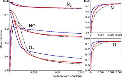
Figure 6: Thermal refinement for Fire II-Testcase B: species mole fractions in the post-shock region; - - - baseline simulation (1$T$); —– Lagrangian simulation (1$T$ $\rightarrow$ $T$-$T^{v}$); $\bm{\cdots}$ reference simulation ($T$-$T^{v}$).

The temperatures obtained by means of the Lagrangian solver follow closely the reference solutions, except for a slight anticipation of the point where translational and internal temperatures cross each other. Concerning the chemical composition, a couple of important points should be highlighted: (1) The Lagrangian solution is improved by at least 40% and approaches the reference result much quicker than the baseline solution; (2) The peak of $\mathrm{NO}$ is slightly anticipated in position but correctly reproduced in amplitude, while it was originally underpredicted by the baseline solution. A correct prediction of this peak is crucial to an accurate calculation of the shock layer radiation.[56]

3.3 State-to-state refinement

We study the excitation and ionization of an argon plasma in the continuum regime past a strong 1D shockwave, using a state-to-state mechanism. The freestream conditions for the shock-tube case studied, representative of an experiment performed at the University of Toronto’s Institute of Aerospace Studies (UTIAS), [57] are given in Table 2.

$V_{\infty}$ [m/s]	$P_{\infty}$ [Pa]	$T_{\infty}$ [K]	$\rm{Ma}_{\infty}$ [-]
5 103	685.3	293.6	15.9

Table 2: Freestream conditions for the UTIAS argon shock-tube experiment (Testcase C).

Two mixtures are considered in this section: a multi-temperature mixture composed of 3 species denoted by the set $\mathcal{S}_{3}=\{\mathrm{Ar}$, $\mathrm{Ar}^{+}\!\!\!$, $\mathrm{e}^{-}\}$, so-called “argon-3,” and a state-to-state mixture composed of 34 species denoted by the set $\mathcal{S}_{34}=\{\mathrm{Ar(i)}~{}|~{}(i=1,\ldots,31)$, $\mathrm{Ar}^{+}(1)$, $\mathrm{Ar}^{+}(2)$, $\mathrm{e^{-}}\}$, so-called “argon-34.” The initial composition is assumed to be in local thermodynamic equilibrium at the freestream conditions.

The solution is recomputed in the post-shock region by means of the Lagrangian reactor using a state-to-state model, starting from a two-temperature ($T$-$T^{e}$) baseline solution, where the translational energy of the heavy-particle bath is at temperature $T$, and the translational energy of electrons and electronic energy of the heavy-particle bath at temperature $T^{e}$, the populations of the electronic energy levels of $\mathrm{Ar}$ and $\mathrm{Ar}^{+}$ following a Boltzmann distribution. The post-shock conditions used for the baseline solution assume that the electron-electronic mode is frozen, so that temperature $T$ jumps, while temperature $T^{e}$ remains at its freestream value. The baseline solution is obtained for the argon-3 mixture by solving in steady conditions the system (1) coupled to eq. (3) for the mode at temperature $T^{e}$. The two temperatures then relax towards each other and eventually equilibrate at the same value. The state-to-state Lagrangian eqs. (15), (20), and (21) presented in Appendix are solved using the argon-34 mixture. Note that two temperatures are considered in the state-to-state case: the heavy-particle translational temperature $T$ and the electron translational temperature $T_{e}$. A reference solution is obtained for the argon-34 mixture by solving in steady conditions the system (1) coupled to the electron energy eq. (2).

The chemical mechanism and rate coefficients for the argon-34 mixture follow Kapper and Cambier’s recommendations. [46] The chemical mechanism for the argon-3 mixture comprises electron-impact ionization [58] and atom-impact ionization. The forward rate coefficient $k_{f}(T^{e})=A~{}(T^{e})^{n}\exp(-T_{0}/T^{e})$ for argon-impact ionization is obtained by integrating experimental cross-section data[59] and is subsequently multiplied by a scaling factor to retrieve the thermal equilibrium point of the reference state-to-state temperature profile, as reported in Table 3. Backward rate coefficients are computed from the equilibrium constant imposing micro-reversibility.

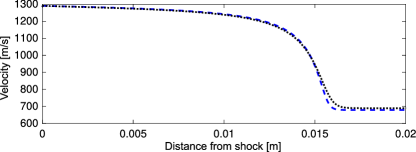
Figure 7: State-to-state refinement for UTIAS-Testcase C: velocity in the post-shock region; - - - baseline simulation (argon-3); $\bm{\cdots}$ reference simulation (argon-34).

$A$ [$\mathrm{cm}^{3}/\mathrm{s}\,\mathrm{mol}$]	$n$ [–]	$T_{0}$ [K]
$1.8247\times 10^{-6}$	$3.597$	69 940

Table 3: Arrhenius parameters for forward rate coefficient of argon atom-impact ionization reaction.

The reference state-to-state flowfield is matched with good accuracy, as shown in Fig. 7. The baseline solution is recomputed using the Lagrangian reactor with the state-to-state approach. Owing to the fidelity of the baseline flowfield, the Lagrangian simulation provides temperatures very close to the reference solution (Fig. 8) and a complete matching in terms of argon electronic energy population. In fact, if the exact flow velocity and density would be used as an input for the Lagrangian solver, the exact solution would be retrieved, by consistency of the equations.

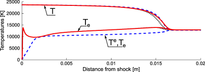
Figure 8: State-to-state refinement for UTIAS-Testcase C: heavy-particle translational temperature, electronic temperature and electron translational temperature in the post-shock region; - - - baseline simulation (argon-3); —– Lagrangian simulation (argon-3 $\rightarrow$ argon-34); $\bm{\cdots}$ reference simulation (argon-34).

3.4 2D rarefied flows

We study the excitation and ionization of an argon plasma past a bow shockwave in the rarefied regime in two parts. In Part 1, as a proof of concept, the Lagrangian solver is first used on a baseline simulation obtained by means of the Direct Simulation Monte Carlo method for a single-species argon gas without considering its internal energy. The first goal is to test the Lagrangian approach against a multidimensional flow around a cylinder, using the decoupled single-streamline mode introduced in section 2.3. The second goal is to demonstrate that the solver (which is hydrodynamic in nature) can tackle the rarefied regime, importing enthalpy variations from the baseline simulation. In Part 2, the Lagrangian solver is run for the argon-34 mixture using a collisional-radiative mechanism.

The DSMC method [39] is a particle-based approach for solving the Boltzmann equation. The result is thus valid even at high rarefaction degrees. Additionally, the stochastic nature of DSMC provides an independent verification of our Lagrangian tool based on a (deterministic) partial differential equation formulation. Argon is an inert gas chosen to test the “rarefaction capabilities” of the Lagrangian solver, with no interference of the chemical refinement procedure. Three baseline solutions are obtained at different Knudsen numbers in the transition regime, using the DSMC software SPARTA. [60] Table 4 shows the freestream velocity $V_{\infty}$, temperature $T_{\infty}$, Mach number $\rm{Ma}_{\infty}$, body diameter $d$, and wall temperature $T_{wall}$ taken from Lofthouse.[61] The Knudsen numbers based on a cylinder of diameter $d$ are obtained by adopting different freestream number densities, as shown in Table 5. Baseline simulations temperature fields are shown in Fig. 9. For a constant Mach number, the shock progressively exhibits a more diffuse behavior for higher values of the Knudsen number.

	$V_{\infty}$ [m/s]	$T_{\infty}$ [K]	$\rm{Ma}_{\infty}$ [–]	$d$ [m]	$T_{wall}$ [K]
$i)$	2 624	200	10	0.304	500
$ii)$	6 585	300	25	0.304	1500

Table 4: Freestream conditions for argon flow around cylinder (Testcase D). $i)$: conditions for Part 1. $ii)$: conditions for Part 2.

	$\mathrm{Kn}_{d}$ [–]	$n_{\infty}$ [1/m3]
case (a)	0.01	$4.247\times 10^{20}$
case (b)	0.05	$8.494\times 10^{19}$
case (c)	0.25	$1.699\times 10^{19}$

Table 5: Knudsen numbers and number densities for argon flow around cylinder (Testcase D).

Part 1. Starting from the baseline solution, the velocity and density fields are extracted along the stagnation line and fed to the Lagrangian reactor. The Lagrangian eqs.  (15) and (22) given in Appendix are solved to recompute the temperature as a verification step. Two alternative cases are studied: an adiabatic Lagrangian simulation obtained by setting the term $\Delta H^{*}/\Delta s=0$ in eq. (22), and a Lagrangian simulation using the baseline enthalpy dissipation obtained by importing this term from the baseline solution. In the former case, the Lagrangian solver cannot reproduce the temperature field close to the wall, as shown in Fig. 10. Due to the purely hyperbolic nature of the adiabatic formulation, the marching approach updates the solution based only on previous streamline points, and contains no information over the upcoming wall temperature. Instead, the adiabatic simulation allows us to retrieve the total temperature value at the stagnation point. This result complies with the nature of adiabatic flows, where there can be no energy exchange with surfaces. When the heat flux is imported from the baseline simulation, the correct solution can be retrieved exactly. Analogous simulations were performed on side streamlines other than the stagnation line, retrieving the very same degree of accuracy.

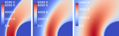
Figure 9: Argon flow around cylinder (Testcase D), baseline DSMC temperature field. Left: case (a) Kn =0.01; middle: case (b) Kn=0.05; right: case (c) Kn=0.25.

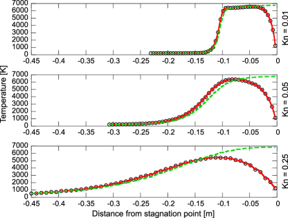
Figure 10: Argon flow around cylinder (Testcase D), temperature along stagnation line; $\circ\!\circ\!\circ$ baseline DSMC simulation; - - - adiabatic Lagrangian simulation; —– Lagrangian simulation using baseline enthalpy dissipation.

This testcase shows that the solver behaves well in rarefied multidimensional single-species flows. The capability of importing the enthalpy from the baseline solution allows us to correctly reproduce heat fluxes even in rarefied conditions, as long as they are considered consistently with the simulated regime. Likewise, this capability proves to be crucial to study continuum flows with temperature gradients, where it is important to reproduce the heat exchange with nearby fluid elements.

As long as specific closures are not introduced for the diffusion terms, the governing equations solved with the Lagrangian approach are general and fully equivalent to mass, momentum and energy balances. Their range of validity over different rarefaction regimes thus depends on the validity of energy fluxes themselves. By importing the energy flux from the baseline DSMC solution, we can guarantee that they comply with the rarefaction degree of the case considered. In this testcase, since no new species are introduced in the computation, the DSMC fluxes are not only accurate, but numerically exact, giving a perfect matching of the solutions. A different approach consists in computing the heat fluxes, using for example Fourier’s law, valid in the continuum approach, as it will be detailed in Testcase E. In a multi-species flow, not only energy but also mass diffusion needs to be modeled: importing the diffusive mass fluxes from the baseline solution is not feasible when chemical refinement is performed, since it introduces additional chemical species whose diffusion velocity is unknown a priori. An option is using continuum modeling for the mass fluxes, as shown in Testcase E.

Part 2. At this point, a further computation is performed, to mimic a possible application. A DSMC computation is performed at $\rm{Kn}=0.01$ at higher freestream velocity, see Table 4, in order to reach higher post-shock temperatures. The computation is refined with a state-to-state approach, additionally enabling radiation compared to Testcase C. The approach consists in solving mass eq. (15), electron temperature eq. (23) and temperature eq. (24) like in Testcase C. Total enthalpy variation is the only diffusive process accounted for, by importing quantity $\Delta H^{*}/\Delta s$ from the baseline DSMC computation. The details of the source and radiation terms can be found in Kapper and Cambier.[46] The temperature profiles are shown in Fig. 11. The DSMC simulation accounts for ground state argon only: this explains the difference in translational temperature between the baseline and Lagrangian simulations, where part of the energy is transfered to the excited electronic energy levels and the free electrons. In Fig. 12, the populations of the argon electronic energy levels are shown along the stagnation line. They are normalized with respect to ground state as follows $\log[(g_{{\rm Ar}(1)}Y_{{\rm Ar}(i)})/(g_{{\rm Ar}(i)}Y_{{\rm Ar}(1)})]$, where quantity $g_{{\rm Ar}(i)}$ stands for the degeneracy of level $i$. Populations are seen to be non-Boltzmann. The effect of radiation is apparent for this case: the non-radiative case reaches equilibrium quicker along the shock, while radiation lowers the proportion of highly excited argon atoms, in favor of lower ones. It is clear that by enabling radiation, higher energy levels decay into lower energy ones, in the high-temperature post shock region.

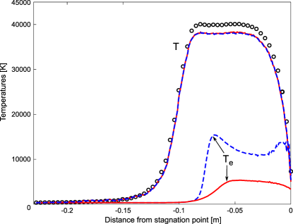
Figure 11: Argon flow around cylinder (Testcase D, Kn $=0.01$), heavy-particle and electron translational temperatures along the stagnation line. $\circ\!\circ\!\circ$ Baseline DSMC solution; - - - radiation disabled; —– radiation enabled.

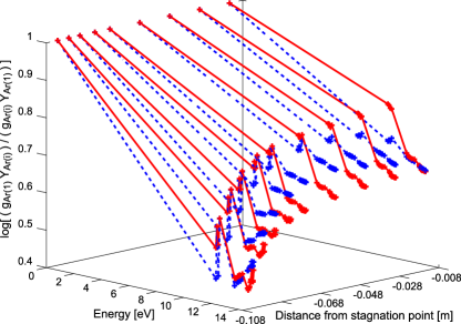
Figure 12: Argon flow around cylinder (Testcase D, Kn $=0.01$), state-to-state population of argon electronic energy levels (logarithmic scale) normalized with respect to ground state along the stagnation line. - - - Radiation disabled; —– Radiation enabled.

3.5 Mass and energy diffusion

We study ionization-recombination processes in air for the rarefied regime, as well as mass and energy diffusion of electrons, along the trail past a blunt body moving at hypersonic speed. This is the most inclusive among the testcases studied, combining chemical refinement with rarefaction and diffusion capabilities in a multidimensional flow. Considering a 2D axisymmetric flow past a spheric body, mass and energy fluxes are modeled in the transversal direction, allowing us to assess the coupled multi-streamlines mode introduced in section 2.3. Table 6 shows the freestream velocity $V_{\infty}$, pressure $P_{\infty}$, temperature $T_{\infty}$, Mach number $\rm{Ma}_{\infty}$, body diameter $d$, and wall temperature $T_{\mathrm{wall}}$. The main idea behind this testcase is to include in the Lagrangian simulation elementary processes absent from the DSMC simulation, $i.e.$, reactions of electron-ion recombination.

$V_{\infty}$ [m/s]	$P_{\infty}$ [Pa]	$T_{\infty}$ [K]	$\rm{Ma}_{\infty}$ [–]	$d$ [m]	$T_{\mathrm{wall}}$ [K]
20 000	3.61	220	67.3	0.01	2000

Table 6: Freestream conditions for partially ionized air trail past a blunt body (Testcase E).

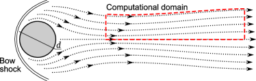
Figure 13: Computational domain for blunt body trail problem (Testcase E); out of scale.

Considering a freestream Knudsen number $\mathrm{Kn}\approx 0.1$ (based on the body diameter), the baseline solution is obtained using the SPARTA software, for a chemically reacting air-11 mixture. The DSMC method used inherently includes mass and energy diffusion but the chemical mechanism employed does not take into account recombination reactions. First, we present a verification step by recomputing the composition by means of the Lagrangian solver using the same chemical mechanism as in the baseline simulation, excluding recombination. A number of streamlines are extracted from the baseline solution in the trail region. The computational domain, sketched in Fig. 13, starts $2$ diameters after the rear stagnation point and extends for $32.5$ diameters. The upper side is limited by the upper streamline and the lower by the axis (coinciding with the lower streamline). Dimensions are reported in Fig. 14. The eqs. (16) and (25) solved are given in Appendix. Transverse diffusion is modeled by means of a continuum closure: multicomponent diffusion for the species mass fluxes and Fourier’s law together with enthalpy diffusion for the mixture heat flux.[36] The simulation is based on the coupled multi-streamlines mode, picking the initial conditions from the first point of each streamline. A number of $25$ streamlines was found to be enough to reproduce accurately the baseline electron concentration.

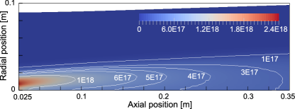
Figure 14: Partially ionized air trail past a blunt body (Testcase E): electron number density field for the Lagrangian simulation. Recombination included.

The radial electron density at the exit of the domain is compared to the baseline simulation in Fig. 15, showing a good agreement. The statistical scatter present in the DSMC solution is mainly due to the low density of free electrons, considering that the ionization degree at the exit is of the order of $0.01\%$. In principle, a longer sampling time would reduce the scatter. Note also that the noise is higher near the axis, due to the strong reduction of the cell size in axisymmetric configuration, resulting in even less simulated particles. The near-axis outlier points are to be considered a numerical artifact.

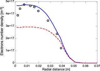
Figure 15: Partially ionized air trail past a blunt body (Testcase E): radial electrons number density at 0.35 m; $\circ\circ\circ$ baseline DSMC simulation; —– Lagrangian simulation without recombination; - - - Lagrangian simulation with recombination.

The Lagrangian solver is then applied to include recombination reactions a posteriori in the chemical mechanism. The recomputed number density field of free electrons is reported in Fig. 14. As expected, the electron number density is significantly reduced, as shown in Fig. 15. The effect of free electrons diffusion over recombination can be easily assessed, by enabling or disabling the respective terms in the equations. Figure 16 shows that diffusion prevails over recombination at these conditions as quantified by computing the third Damköhler number, ratio of the diffusive-over-reactive timescale. Its value is $\rm{Da_{\rm{III}}}=\tau^{\mathrm{diff}}/\tau^{\mathrm{react}}\approx 10^{-8}$.

Despite the degree of rarefaction, particles have enough time to thermalize moving along the trail. For this reason, recomputing fluxes using the continuum assumption works well in this testcase. In fact, sampling the velocity distributions function from the DSMC simulation gives quasi-Maxwellian shapes. The Knudsen number in this problem would indeed result much smaller if, as a reference length, one would choose the distance along the axis. The Lagrangian approach brings a number of advantages. First, the numerical scatter of minor species is reduced, naturally improving the accuracy of the chemical reactions prediction (and radiation if included). Second, one could perform lighter DSMC simulations by reducing the number of species and performing a computationally efficient refinement a posteriori with a large number of species. Particular reactions not yet implemented in a DSMC code can be easily introduced as well.

Finally, regarding blunt body trail simulations, it is possible to use the Lagrangian reactor to obtain solutions up to extremely long distances from the body. In fact, in rarefied conditions velocity and density often reach freestream values, while free electrons are still not totally recombined. This feature allows us to obtain baseline solutions that would be too expensive to achieve by means of the DSMC method: the trail is extended assuming straight streamlines with freestream values for velocity and density. Taking the results obtained above as an initial condition, the Lagrangian solver was used to study the evolution of free electrons in the trail up to $0.05$ seconds after the body passage, equivalent to a trail length of 1 km, $i.e.\ 10\,000$ times the body diameter. Figure 17 shows the persistence of free electrons in the trail. The simulation by means of the Lagrangian solver takes around 20 minutes on a laptop. On the other hand, a full DSMC simulation of the same domain would be extremely heavy, requiring to simulate around $10^{9}$ particles and $250$ million cells in order to meet the DSMC convergence criteria.[39]

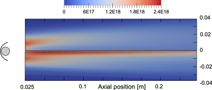
Figure 16: Partially ionized air trail past a blunt body (Testcase E): effect of diffusion of free electrons versus recombination reactions. Electron number density [m^-3] for the Lagrangian simulation: top, only diffusion; bottom, only recombination. Meteoroid included in scale for dimensional comparison.

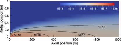
Figure 17: Partially ionized air trail past a blunt body (Testcase E): electron number density [m^-3] for the Lagrangian simulation based on extrapolated baseline simulation in a 1 km trail. Axis not in scale.

4 Conclusions

In this work, we discussed the development and testing of a diffusive Lagrangian solver allowing us to compute the thermochemical state of reactive and plasma flows. Starting from a baseline solution obtained with any analytical, numerical, or even experimental methods, the Lagrangian solver can be used to introduce an arbitrarily large number of chemical species and their related chemical mechanism, together with a specific treatment of the internal energy based on multi-temperature or state-to-state models. The governing equations are solved along the streamlines, importing the velocity and density fields directly from the baseline solution, carrying the information over the original problem geometry. The Lagrangian solver recomputes the chemical species concentration and the temperature fields, for both the single and multiple streamlines modes developed. The single-streamline mode was formulated in such a way that dissipative fluxes of energy can be externally introduced in the formulation. This allowed us to extend the validity of the method to rarefied conditions by considering a baseline solution obtained by means of the DSMC method. For the multi-streamline mode, a finite-volume method was proposed to compute the transverse mass and energy diffusive fluxes.

The Lagrangian solver was assessed for a number of testcases. First, the chemical and thermal refinement capabilities were examined using multi-temperature models, studying the thermochemical relaxation past a 1D strong shockwave in an air mixture. The test was repeated for an argon mixture, employing a state-to-state collisional-radiative model. The approach was then tested on multidimensional cases, studying a 2D argon flow over a cylinder in the transition regime, then moving to the simulation of a chemically reacting air trail past a blunt body in 2D axisymmetric geometry, computing mass and energy diffusion across streamlines.

For all the testcases studied, the solver developed was used to estimate the effects of a detailed chemistry or thermal nonequilibrium on a baseline simulation. The results demonstrate that the method developed enables coupling detailed mechanisms to multidimensional solvers to study thermo-chemical nonequilibrium flows. One should notice that the imported velocity and density fields appear in the Lagrangian equations through the mass flux $\rho U$ and kinetic energy flux $U^{3}$. While the former is constant along each streamline, the latter may change according to the thermochemical model adopted. In particular, when minor species are introduced using the Lagrangian reactor, these species can be thought as transported scalars, not altering significantly the energy balance of the mixture. The simplified velocity field is found to be very close to the one obtained for the full mixture, and the Lagrangian solver provides very accurate solutions. More care should be paid when newly introduced minor species play an important role in the chemical mechanism, or when the coarse thermochemical model is too poor to describe correctly the baseline solution, in terms of hydrodynamic features. The Lagrangian reactor can always be tested on simplified representative problems, to assess which accuracy can be expected for the real problem. Nonetheless, in all the testcases performed, the Lagrangian reactor improved drastically the baseline simulations. The computational cost of a Lagrangian recomputation is typically orders of magnitude smaller with respect to a full solution of the problem. The solver has the additional benefit of being immune from statistical noise, which strongly affects the accuracy of DSMC simulations, especially considering minor species in the mixture.

A number of applications can be tackled with the method developed, ranging from the interpretation of measurement techniques such as optical emission spectroscopy to design of plasma generators. The testcase performed suggests applications in the refinement of the temperature profile past shock waves, and the estimation of radiative properties employing collision-radiative models. The calculation of the free electron concentration in hypersonic trails was also discussed in this paper, which can easily be applied to the fields of telecommunication blackout and the radio-detection of meteors during atmospheric entry.[62, 63] Extended trail simulations of meteors is an ongoing work performed by means of the Lagrangian solver, including ablation products. [64]

Appendix

We consider a system of elementary reactions $r\in\mathcal{R}$ formally written as

$$\sum_{i\in\mathcal{S}}\nu^{{}^{\prime}}_{ir}X_{i}\rightleftharpoons\sum_{i\in\mathcal{S}}\nu^{{}^{\prime\prime}}_{ir}X_{i},$$

where $X_{i}$ is the chemical symbol for species $i\in\mathcal{S}$, and $\nu^{{}^{\prime}}_{ir}$ and $\nu^{{}^{\prime\prime}}_{ir}$, the forward and backward stoichiometric coefficients for species $i$ in reaction $r$. The species production rates, compatible with the law of mass action, are expressed as $\omega_{i}=M_{i}\sum_{r\in\mathcal{R}}\nu_{ir}\tau_{r}$, where $\nu_{ir}=\nu^{{}^{\prime\prime}}_{ir}-\nu^{{}^{\prime}}_{ir}$ and symbol $M_{i}$ stands for the species molar mass. The rate of progress for reaction $r$ is given by:

$$\tau_{r}=k_{r}^{f}\prod_{i\in\mathcal{S}}\left(\frac{\rho_{i}}{M_{i}}\right)^{\nu^{{}^{\prime\prime}}_{ir}}-k_{r}^{b}\prod_{i\in\mathcal{S}}\left(\frac{\rho_{i}}{M_{i}}\right)^{\nu^{{}^{\prime}}_{ir}}.$$

The mass conservation equations solved for the test cases of Section 3 are given as follows.

Testcases A, B, C, and D

$$\frac{\mathrm{d}Y_{i}}{\mathrm{d}s}=\frac{\omega_{i}}{\rho U},\quad i\in\mathcal{S},$$ (15)

Testcase E

$$\frac{\partial Y_{i}}{\partial x}+\frac{1}{\rho U\,\cos{\alpha_{k}}}\frac{\partial J_{i}}{\partial r}=\frac{\omega_{i}}{\rho U\,\cos{\alpha_{k}}},\quad i\in\mathcal{S},$$ (16)

where index $k$ refers to the streamline considered. The transverse mass flux is $J_{i}=\rho_{i}V_{i}$, where the diffusion velocity $V_{i}=-\sum_{j\in\mathcal{S}}$ $D_{ij}{\partial}X_{j}/{\partial r}+\rho_{i}q_{i}E/(m_{i}P)$ depends on the transverse gradients of species mole fractions $X_{i}$, through multicomponent diffusion coefficients $D_{ij}$, and the (ambipolar) electric field $E$, where $q_{i}$ is the charge of species $i$ and $m_{i}$ its mass.

The energy conservation equations solved for the testcases of Section 3 are given as follows.

Testcase A

$$\frac{\mathrm{d}T}{\mathrm{d}s}=-\left[\tfrac{1}{3}\rho\frac{\mathrm{d}U^{3}}{\mathrm{d}s}+\sum_{j\in\mathcal{S}}{h_{j}\omega_{j}}\right]\Bigg{/}\left[{\rho U}\sum_{j\in\mathcal{S}}c_{p,j}Y_{j}\right],$$ (17)

Testcase B

$$\frac{\mathrm{d}T^{v}}{\mathrm{d}s}=\left[{\Omega^{v,e}}-\sum_{j\in\mathcal{H}}{e^{v,e}_{j}\omega_{j}}\right]\Bigg{/}\left[{\rho U}\sum_{j\in\mathcal{H}}c_{v,j}^{v,e}Y_{j}\right],$$ (18)

$$\frac{\mathrm{d}T}{\mathrm{d}s}=-\left[\tfrac{1}{3}\rho\frac{\mathrm{d}U^{3}}{\mathrm{d}s}+\sum_{j\in\mathcal{H}}{h_{j}\omega_{j}}\right.\\ \left.+\left(\Omega^{v,e}-\sum_{j\in\mathcal{H}}e_{j}^{v,e}\omega_{j}\right)\right]\Bigg{/}\left[{\rho U}\sum_{j\in\mathcal{H}}c_{p,j}^{t,r}Y_{j}\right],$$ (19)

where the source term for the vibrational-translational energy relaxation (Landau-Teller-Millikan-White) and chemistry-energy coupling is introduced as follows,[44] $\Omega^{v,e}=\sum_{j\in\mathcal{H}}\rho_{j}[{e^{v}_{j}\left(T\right)-e^{v}_{j}\left(T^{v}\right)}]/{\tau_{j}^{VT}}+\sum_{j\in\mathcal{H}}e^{v,e}_{j}\omega_{j}$.

Testcase C

$$\frac{\mathrm{d}T_{e}}{\mathrm{d}s}=\left[\Omega_{e}+\frac{P_{e}U}{\rho}\frac{\mathrm{d}\rho}{\mathrm{d}s}-e^{t}_{e}\omega^{e}\right]\Big{/}\left[\phantom{\frac{\mathrm{d}\rho}{\mathrm{d}s}}{\rho U}c_{v,e}Y_{e}\right],$$ (20)

$$\frac{\mathrm{d}T}{\mathrm{d}s}=-\left[\tfrac{1}{3}\rho\frac{\mathrm{d}U^{3}}{\mathrm{d}s}+\sum_{j\in\mathcal{S}}{h_{j}\omega_{j}}+{\gamma_{e}}\left(\Omega_{e}\vphantom{\frac{P_{e}U}{\rho}}+\frac{P_{e}U}{\rho}\frac{\mathrm{d}\rho}{\mathrm{d}s}\right.\right.\\ \left.\left.\vphantom{\frac{\mathrm{d}\rho}{\mathrm{d}s}}-e_{e}^{t}\omega_{e}\right)\vphantom{\sum_{j}}\right]\Bigg{/}\left[{\rho U}\sum_{j\in\mathcal{H}}c_{p,j}^{t}Y_{j}\right],$$ (21)

where the source term for the electron heavy-particle translational energy transfer and chemistry-energy coupling is introduced as follows,[44] $\Omega_{e}=\rho_{e}[{e^{T}_{e}\left(T\right)-e^{T}_{e}\left(T_{e}\right)}]/{\tau^{ET}}+\sum_{r\in\mathcal{R}^{\star}}\Delta h^{r}\tau^{r}+e^{t}_{e}\omega^{e}$. The set $\mathcal{R}^{\star}\subset\mathcal{R}$ comprises the electron-impact ionization and excitation reactions.

Testcase D

Part 1: Thermal equilibrium case

$$\frac{\mathrm{d}T}{\mathrm{d}s}=\left[\vphantom{\sum_{j}}\frac{\Delta H^{*}}{\Delta s}-\tfrac{1}{2}\frac{\mathrm{d}U^{2}}{\mathrm{d}s}\right]\Bigg{/}\left[\sum_{j\in\mathcal{S}}c_{p,j}Y_{j}\right],$$ (22)

Part 2: Collisional-radiative model case

$$\frac{\mathrm{d}T_{e}}{\mathrm{d}s}=\left[\Omega_{e}+\mathscr{P}_{e}+\frac{P_{e}U}{\rho}\frac{\mathrm{d}\rho}{\mathrm{d}s}-e^{t}_{e}\omega_{e}\right]\Big{/}\left[\rho U\,c_{v,e}^{t}Y_{e}\vphantom{\frac{P_{e}U}{\rho}}\right],$$ (23)

$$\frac{\mathrm{d}T}{\mathrm{d}s}=\left[{\rho U}\frac{\Delta H^{*}}{\Delta s}+{\mathscr{P}}-\tfrac{1}{3}\rho\frac{\mathrm{d}U^{3}}{\mathrm{d}s}-\sum_{j\in\mathcal{S}}{h_{j}\omega_{j}}-{\gamma_{e}}\left(\Omega_{e}\phantom{\frac{P_{e}U}{\rho}}\right.\right.\\ \left.\left.+\mathscr{P}_{e}-\frac{P_{e}U}{\rho}\frac{\mathrm{d}\rho}{\mathrm{d}s}-e_{e}^{t}\omega_{e}\right)\phantom{\sum_{j}}\right]\Bigg{/}\left[\rho U\sum_{j\in\mathcal{H}}c_{p,j}^{t}Y_{j}\right],$$ (24)

where $\mathscr{P}=-\sum_{(i,j)\in\mathcal{S}^{BB}}\Lambda_{ij}(h_{j}^{f}-h_{i}^{f})n_{j}A_{ji}$ expresses energy lost through bound-bound transitions from an upper electronic energy level $j$ of argon to a lower level $i$, denoted by the set $\mathcal{S}^{BB}$, with the escape factors assumed to be $\Lambda_{ij}=0$ for transitions to the ground state (optically thick) and $1$ for all the others (optically thin); and $A_{ji}$ the Einstein coefficient for the transition. The term $\mathscr{P}_{e}=\sum_{i\in\mathcal{S}_{31}}(h^{f}_{{\rm Ar}^{+}}-h^{f}_{i})n_{i}R_{i}$ $-1.42\times 10^{-40}Z_{\mathrm{eff}}^{2}T_{e}^{1/2}n_{{\rm Ar}^{+}}n_{e}~{}[{\rm W}/{\rm m}^{3}]$ accounts for photorecombination with rate coefficient $R_{i}$, where $\mathcal{S}_{31}=\{\mathrm{Ar(i)}~{}|~{}(i=1,\ldots,31)\}$, and Bremsstrahlung with an effective charge $Z_{\mathrm{eff}}^{2}=1.67$.[65]

Testcase E

$$\frac{\partial T}{\partial x}+\left[\frac{\partial q}{\partial r}-\sum_{j\in\mathcal{S}}h_{j}\left(\frac{\partial J_{j}}{\partial r}\right)\right]\Bigg{/}\left[\rho U\,\cos{\alpha_{k}}\sum_{j\in\mathcal{S}}c_{p,j}Y_{j}\right]\\ =-\left[\tfrac{1}{3}\rho\frac{\partial U^{3}}{\partial s}+\sum_{j\in\mathcal{S}}h_{j}\omega_{j}\right]\Bigg{/}\left[\rho U\,\cos{\alpha_{k}}\sum_{j\in\mathcal{S}}c_{p,j}Y_{j}\right],$$ (25)

where $k$ is the index of streamline considered. The mass flux $J_{i}$, $i\in\mathcal{S}$ is defined as in eq. (16). The transverse heat flux is introduced as $q=-\lambda\frac{\partial}{\partial r}T+\sum_{j\in\mathcal{S}}h_{j}J_{j}$, where $\lambda$ is the thermal conductivity.

References

- [1] George Raiche and David Driver. Shock Layer Optical Attenuation and Emission Spectroscopy Measurements During Arc Jet Testing with Ablating Models. In 42nd AIAA Aerospace Sciences Meeting and Exhibit. American Institute of Aeronautics and Astronautics, 2018.
- [2] Gregory P. Smith, David M. Golden, Michael Frenklach, Nigel W. Moriarty, Boris Eiteneer, Mikhail Goldenberg, C. Thomas Bowman, Ronald K. Hanson, Soonho Song, William C. Jr. Gardiner, Vitali V. Lissianski, and Zhiwei Qin. GRI-Mech 3.0.
- [3] N. A. Popov. Kinetics of plasma-assisted combustion: effect of non-equilibrium excitation on the ignition and oxidation of combustible mixtures. Plasma Sources Science and Technology, 25(4):043002, 2016.
- [4] S. Kobayashi, Z. Bonaventura, F. Tholin, N. Popov, and A. Bourdon. Study of nanosecond discharges in h2-air mixtures at atmospheric pressure for plasma assisted combustion applications. Plasma Sources Science and Technology, 26:075004, 2017.
- [5] John Cooper. Plasma spectroscopy. Reports on Progress in Physics, 29(1):35, 1966.
- [6] C. O. Laux, T. G. Spence, C. H. Kruger, and R. N. Zare. Optical diagnostics of atmospheric pressure air plasmas. Plasma Sources Science and Technology, 12:125–138, 2003.
- [7] Yana G. Maneva, Alejandro Alvarez Laguna, Andrea Lani, and Stefaan Poedts. Multi-fluid modeling of magnetosonic wave propagation in the solar chromosphere: Effects of impact ionization and radiative recombination. The Astrophysical Journal, 836(2):197, 2017.
- [8] Alessandro Munafò, Nagi N. Mansour, and Marco Panesi. A reduced-order nlte kinetic model for radiating plasmas of outer envelopes of stellar atmospheres. The Astrophysical Journal, 838(2):126, 2017.
- [9] A. V. Bulgakov and N. M. Bulgakova. Gas-dynamic effects of the interaction between a pulsed laser-ablation plume and the ambient gas: analogy with an underexpanded jet. Journal of Physics D: Applied Physics, 31(6):693, 1998.
- [10] R. J. Shul, G. B. McClellan, R. D. Briggs, D. J. Rieger, S. J. Pearton, C. R. Abernathy, J. W. Lee, C. Constantine, and C. Barratt. High-density plasma etching of compound semiconductors. Journal of Vacuum Science & Technology A, 15(3):633–637, 1997.
- [11] D. M. Sanders, D. B. Boercker, and S. Falabella. Coating technology based on the vacuum arc-a review. IEEE Transactions on Plasma Science, 18(6):883–894, Dec 1990.
- [12] Bernd Helber. Material Response Characterization of Low-density Ablators in Atmopheric Entry Plasmas. PhD Thesis, von Karman Institute for Fluid Dynamics and Vrije Universiteit Brussel, Brussels, Belgium, 2016.
- [13] Jeff C. Taylor, Ann B. Carlson, and H. A. Hassan. Monte Carlo simulation of radiating re-entry flows. Journal of Thermophysics and Heat Transfer, 8(3):478–485, 1994.
- [14] Chul Park. Review of chemical-kinetic problems of future NASA missions. I - Earth entries. Journal of Thermophysics and Heat Transfer, 7(3):385–398, 1993.
- [15] Chul Park, John T. Howe, Richard L. Jaffe, and Graham V. Candler. Review of chemical-kinetic problems of future NASA missions. II - Mars entries. Journal of Thermophysics and Heat Transfer, 8(1):9–23, 1994.
- [16] Vivien Croes, Trevor Lafleur, Zdeněk Bonaventura, Anne Bourdon, and Pascal Chabert. 2d particle-in-cell simulations of the electron drift instability and associated anomalous electron transport in hall-effect thrusters. Plasma Sources Science and Technology, 26(3):034001, 2017.
- [17] Jason D. Sommerville, Lyon B. King, Yu-Hui Chiu, and Rainer A. Dressler. Ion-collision emission excitation cross sections for xenon electric thruster plasmas. Journal of Propulsion and Power, 24(4):880–888, 2008.
- [18] Arnaud Bultel, Bruno G. Chéron, Anne Bourdon, Ousmanou Motapon, and Ioan F. Schneider. Collisional-radiative model in air for earth re-entry problems. Physics of Plasmas, 13(4):043502, April 2006.
- [19] A. Munafò, A. Lani, A. Bultel, and M. Panesi. Modeling of non-equilibrium phenomena in expanding flows by means of a collisional-radiative model. Physics of Plasmas, 20(7):073501, 2013.
- [20] Galina Chaban, Richard Jaffe, David W. Schwenke, and Winifred Huo. Dissociation cross sections and rate coefficients for nitrogen from accurate theoretical calculations. AIAA paper, 1209:2008, 2008.
- [21] Arnaud Bultel and Julien Annaloro. Elaboration of collisional–radiative models for flows related to planetary entries into the earth and mars atmospheres. Plasma Sources Science and Technology, 22(2):025008, 2013.
- [22] L. D. Pietanza, G. Colonna, A. Laricchiuta, and M. Capitelli. Non-equilibrium electron and vibrational distributions under nanosecond repetitively pulsed CO discharges and afterglows: II. the role of radiative and quenching processes. Plasma Sources Science and Technology, 27(9):095003, 2018.
- [23] Hai P. Le, Ann R. Karagozian, and Jean-Luc Cambier. Complexity reduction of collisional-radiative kinetics for atomic plasma. Physics of Plasmas, 20(12):123304, December 2013.
- [24] T. R. Young and J. P. Boris. A numerical technique for solving stiff ordinary differential equations associated with the chemical kinetics of reactive-flow problems. The Journal of Physical Chemistry, 81(25):2424–2427, December 1977.
- [25] Douglas A. Schwer, Pisi Lu, and William H. Green. An adaptive chemistry approach to modeling complex kinetics in reacting flows. Combustion and Flame, 133(4):451–465, June 2003.
- [26] M.Duarte, M. Massot, S. Descombes, C. Tenaud, T. Dumont, V. Louvet, and F. Laurent. New resolution strategy for multiscale reaction waves using time operator splitting, space adaptive multiresolution, and dedicated high order implicit/explicit time integrators. SIAM Journal on Scientific Computing, 34:A76–A104, 2012.
- [27] A. Bellemans, A. Munafò, T. E. Magin, G. Degrez, and A. Parente. Reduction of a collisional-radiative mechanism for argon plasma based on principal component analysis. Physics of Plasmas, 22(6):062108, June 2015.
- [28] A. Munafò, M. Panesi, and T. E. Magin. Boltzmann rovibrational collisional coarse-grained model for internal energy excitation and dissociation in hypersonic flows. Physical Review E, 89(2):023001, February 2014.
- [29] James C. Keck. Rate-controlled constrained-equilibrium theory of chemical reactions in complex systems. Progress in Energy and Combustion Science, 16(2):125–154, 1990.
- [30] Michele Corbetta, Flavio Manenti, and Carlo Giorgio Visconti. CATalytic – Post Processor (CAT-PP): A new methodology for the CFD-based simulation of highly diluted reactive heterogeneous systems. Computers & Chemical Engineering, 60:76–85, January 2014.
- [31] Venkatramanan Raman, Heinz Pitsch, and Rodney O. Fox. Hybrid large-eddy simulation/Lagrangian filtered-density-function approach for simulating turbulent combustion. Combustion and Flame, 143(1-2):56–78, October 2005.
- [32] T. E. Magin, L. Caillault, A. Bourdon, and C. O. Laux. Nonequilibrium radiative heat flux modeling for the Huygens entry probe. Journal of Geophysical Research: Planets, 111(E7):E07S12, July 2006.
- [33] F. Thivet. Modeling of hypersonic flows in thermal and chemical nonequilibrium. PhD Thesis, Ecole Centrale Paris, Châtenay-Malabry, France. in French, 1992.
- [34] Carlo Cercignani. Rarefied gas dynamics: from basic concepts to actual calculations, volume 21. Cambridge University Press, 2000.
- [35] Iu I. Klimontovich. Kinetic theory of nonideal gas and nonideal plasma. Pergamon Press, 1982.
- [36] Vincent Giovangigli. Multicomponent flow modeling. Modeling and Simulation in Science, Engineering and Technology. Birkhäuser Boston Inc., Boston, MA, 1999.
- [37] T. E. Magin, B. Graille, and M. Massot. Kinetic theory of plasmas: translational energy. Mathematical Models and Methods in Applied Sciences, 19:527–599, 2009.
- [38] J. H. Ferziger and H. G. Kaper. Mathematical Theory of Transport Processes in Gases. North-Holland Publishing Company, 1972.
- [39] G. A. Bird. Molecular Gas Dynamics and the Direct Simulation of Gas Flows. Clarendon, Oxford, 1994.
- [40] Zheng Li, Takashi Ozawa, Ilyoup Sohn, and Deborah A. Levin. Modeling of electronic excitation and radiation in non-continuum hypersonic reentry flows. Physics of Fluids, 23(6):066102, June 2011.
- [41] Walter Guido Vincenti and Charles H. Kruger. Introduction to physical gas dynamics. New York, Wiley, 1965.
- [42] James Clerk Maxwell. IV. On the dynamical theory of gases. Philosophical transactions of the Royal Society of London, 157:49–88, 1867.
- [43] S. Chapman and T.G. Cowling. The Mathematical Theory of Non-uniform Gases: An Account of the Kinetic Theory of Viscosity, Thermal Conduction, and Diffusion in Gases. Cambridge University Press, 1958.
- [44] C. Park. Nonequilibrium Hypersonic Aerothermodynamics. Wiley, 1990.
- [45] J.-M.Orlac’H, V. Giovangigli, T. Novikova, and P. Roca. Kinetic theory of two-temperature polyatomic plasmas. Physica A: Statistical Mechanics and its Applications, 494:503–546, 2018.
- [46] M. G. Kapper and J.-L. Cambier. Ionizing shocks in argon. Part I: Collisional-radiative model and steady-state structure. Journal of Applied Physics, 109(11):113308, June 2011.
- [47] D. Bruno and V. Giovangigli. Relaxation of internal temperature and volume viscosity. Physics of Fluids, 23:093104, 2011.
- [48] John David Anderson. Hypersonic and high temperature gas dynamics. Aiaa, 2000.
- [49] Boost c++ libraries, Accessed: 2018-08-08. https://www.boost.org/.
- [50] J. B. Scoggins and T. E. Magin. Development of MUTATION++: MUlticomponent Thermodynamics And Transport properties for IONized gases library in C++, 11th AIAA/ASME Joint Thermophysics and Heat Transfer Conference. Atlanta, USA, 2014.
- [51] MPP / mutationpp, Accessed: 2018-08-13. https://sync.vki.ac.be/mpp/mutationpp.
- [52] John H Lienhard. A heat transfer textbook. Courier Corporation, 2013.
- [53] Dona L Cauchon. Radiative heating results from the fire ii flight experiment at a reentry velocity of 11.4 kilometers per second. NASA TM X-1402, 6, 1967.
- [54] Marco Panesi, Thierry Magin, Anne Bourdon, Arnaud Bultel, and Olivier Chazot. Fire ii flight experiment analysis by means of a collisional-radiative model. Journal of Thermophysics and Heat Transfer, 23(2):236–248, 2009.
- [55] Chul Park, Richard L. Jaffe, and Harry Partridge. Chemical-kinetic parameters of hyperbolic earth entry. Journal of Thermophysics and Heat transfer, 15(1):76–90, 2001.
- [56] L. Soucasse, J. B. Scoggins, P. Rivière, T. E. Magin, and A. Soufiani. Flow-radiation coupling for atmospheric entries using a hybrid statistical narrow band model. Journal of Quantitative Spectroscopy and Radiative Transfer, 180:55–69, 2016.
- [57] I. I. Glass and W. S. Liu. Effects of hydrogen impurities on shock structure and stability in ionizing monatomic gases. part 1. argon. Journal of Fluid Mechanics, 84:55–77, 1978.
- [58] Julien Annaloro and Arnaud Bultel. Vibrational and electronic collisional-radiative model in air for Earth entry problems. Physics of Plasmas, 21(12):123512, December 2014.
- [59] Howard C. Hayden and Robert C. Amme. Low-energy ionization of argon atoms by argon atoms. Physical Review, 141(1):30–31, 1966.
- [60] Michael A. Gallis, John R. Torczynski, Steven J. Plimpton, Daniel J. Rader, and Timothy Koehler. Direct simulation Monte Carlo: The quest for speed. In AIP Conference Proceedings, volume 1628, pages 27–36. AIP, 2014.
- [61] Andrew J. Lofthouse. Nonequilibrium hypersonic aerothermodynamics using the direct simulation Monte Carlo and Navier-Stokes models. PhD Thesis, Michigan Univ Ann Arbor, 2008.
- [62] J.-M. Wislez. Forward scattering of radio waves off meteor trails. In Proceedings of the International Meteor Conference, 14th IMC, Brandenburg, Germany, 1995, pages 99–117, 1996.
- [63] Herve Lamy. Home - Brams - Aeronomy.be, Accessed: 2018-03-08. http://brams.aeronomie.be/.
- [64] Federico Bariselli, Stefano Boccelli, Thierry Magin, Aldo Frezzotti, and Annick Hubin. Aerothermodynamic modelling of meteor entry flows in the rarefied regime. In 2018 Joint Thermophysics and Heat Transfer Conference, AIAA Aviation Forum. American Institute of Aeronautics and Astronautics, 2018.
- [65] Aurélie Bellemans. Simplified plasma models based on reduced kinetics. PhD Thesis, von Karman Institute for Fluid Dynamics and Université Libre de Bruxelles, Brussels, Belgium, 2017.