Non-Hermitian formalism and nonlinear physics

Abstract

The non-Hermitian formalism is used at present in many papers for the description of open quantum systems. A special language developed in this field of physics which makes it difficult for many physicists to follow and to understand the corresponding papers. We show that the characteristic features of the non-Hermitian formalism are nothing but nonlinearities that may appear in the equations when the Hamiltonian is non-Hermitian. They are related directly to singular points (called mostly exceptional points, EPs). At low level density, they may cause counterintuitive physical results which allow us to explain some puzzling experimental results. At high level density, they determine the dynamics of the system.

I Introduction

The properties of non-Hermitian operators are studied today in many papers. They appear originally in the description of open quantum systems such as mesoscopic devises, which assumed an unprecedented interdisciplinary character. These systems may be defined as consisting of some localized microscopic region that is embedded in an external (natural) environment which is independent of the system. This environment always exists and can never be deleted. It is extended in contrast to the system which is localized.

It is obvious that such a system can be described successfully by means of a projection operator technique: one of the operators projects onto the localized system while another one projects onto the extended environment. Both parts are described, as usual, separately by Hermitian operators. The influence of the other subspace onto the considered one causes, however, the Hamiltonian of the considered subsystem to be non-Hermitian. For details see top ; ropp . Meanwhile, a special language developed in the non-Hermitian quantum physics due to which it is difficult for non-specialists to read and to understand the contents of these papers.

The reason for the special language is objective. It arises from the mathematical problems which are inherent in the formalism of non-Hermitian operators and are unknown and counterintuitive in the formalism of Hermitian operators. Details can be found in e.g. the reviews top ; ropp . Nevertheless, the special features of the notions used in non-Hermitian physics are not unique. They can be related to well-known phenomena as will be shown in the following.

The only difference between a Hermitian operator $H$ and a non-Hermitian operator $\cal H$, which is usually known, is that the eigenvalues $E_{i}$ of $H$ are real while the eigenvalues ${\cal E}_{i}$ of $\cal H$ are usually complex, and only sometimes real. The last case (real eigenvalues) is known to appear in calculations for concrete realistic systems. The corresponding eigenstates are called usually bound states in the continuum wintgen1 ; wintgen2 .

The possible coalescence of two eigenvalues of $\cal H$ that may appear at a certain value of the considered parameter, is almost unknown although it is exactly this property of $\cal H$ that determines the interesting properties of non-Hermitian physics which are not only unexpected but mostly counterintuitive. They allow us to explain different experimental results which remained puzzling in Hermitian quantum physics top ; ropp ; entropy . According to the obtained results, the nature of the parameter may be very different.

The problem that two eigenvalues of a non-Hermitian operator $\cal H$ may coalesce is known in mathematics since many years kato . The coalescence occurs formally at one point, which is called mostly exceptional point (EP). In physical systems, it is however not enough to know the properties of the system at one point. Of interest are rather the properties of the system in a certain finite range of the considered parameter. The influence of the EP can be seen, indeed, in a finite neighborhood around this point as the results of many numerical studies have shown top .

The coalescence of two eigenvalues ${\cal E}_{1,2}$ is different from a possible degeneration of two eigenvalues $E_{1,2}$ of a Hermitian operator $H$. While the two corresponding eigenfunctions $\phi_{1,2}$ of $H$ are always different from one another, the two eigenfunctions $\Phi_{1,2}$ of $\cal H$ are related to one another by the special relation

$$\Phi_{1}\to\pm~{}i~{}\Phi_{2}$$ (1)

which holds true in the very neighborhood of the EP where the two states coalesce. A consequence of the relation (1) is that the phases of the eigenfunctions of $\cal H$ are, generally, not rigid. The wavefunctions of two eigenstates of $\cal H$ are almost orthogonal at large distance (in energy) from one another, and related to one another by (1) in approaching an EP top . This means that close to the EP the two eigenfunctions are proportional. In other words, the eigenfunctions $\Phi_{i}$ behave according to Jordan forms, for details see gurosa .

We will show in the following that most of the new terms introduced and used in the formalism of non-Hermitian operators can be replaced by the term nonlinearity. The best example is the basic concept exceptional point, EP, itself. At the parameter value at which the EP appears, the eigenvalue trajectories of the two states (traced as function of the considered parameter) reverse their orientation and do not cross top . Here,

$${\cal E}_{1}\to~{}\pm~{}i~{}{\cal E}_{2}$$ (2)

holds true for the (complex) eigenvalues ${\cal{E}}_{i}$ of $\cal H$, what corresponds to (1). Such a parametrical change of the two eigenvalue trajectories is impossible if the movement occurs linearly as a function of the considered parameter. The change is possible only by means of a nonlinear term that is involved in the equations describing the trajectories of the eigenvalues as a function of this parameter. As usual, this nonlinearity in the parametrical dependence of the eigenvalue trajectories influences the behavior of the trajectories not only at a certain point (at the EP) but also that in the not too far vicinity.

This fact shows that it is even better to use the expression nonlinearity instead of the notion point (EP). According to the usual understanding, a nonlinearity influences the behavior of the system in a finite parameter range. The notion EP suggests however that all the changes in the behavior of the system appear only at one point. This will, of course, never take place in a realistic physical system.

It should be mentioned here that the notation EP is even somewhat misleading because a single EP has nothing in common with a critical point at which the properties of the system change. The two eigenvalue trajectories move independently of one another beyond the influence of the EP. Changes of the system may appear only under the influence of two and more EPs.

The paper is organized in the following manner. In Sect. II, the non-Hermitian Hamiltonians used in the most commonly used descriptions of quantum systems are given. One of them is a genuine non-Hermitian operator which allows us to study in detail characteristic features of the solutions. Another one is an effective Hamiltonian which is suitable, and often used, in numerical calculations on realistic systems. Additionally, we mention the nonlinear formalism used at high level density. In the following Sect. III, we show numerical results obtained from a calculation with a varying number of states in a certain finite energy window. The results of these calculations illustrate the influence of resonance overlapping onto the results and the role of nonlinearities in the basic equations. The results are summarized and discussed in the last section IV.

II Description of realistic open quantum systems

II.1 Genuine non-Hermitian operator

A genuine description of an open quantum system with two eigenstates of $\cal H$ starts proj10 from

$${\cal H}^{(2)}=\left(\begin{array}[]{cc}\varepsilon_{1}\equiv e_{1}+\frac{i}{2}\gamma_{1}&~{}~{}~{}~{}\omega\\ \omega&~{}~{}~{}~{}\varepsilon_{2}\equiv e_{2}+\frac{i}{2}\gamma_{2}\\ \end{array}\right)\;.$$ (5)

Here, $\varepsilon_{i}$ are the complex eigenvalues of the basic non-Hermitian operator $\cal H$ comment1 . The $\omega$ stand for the coupling matrix elements of the two states via the common environment. Their mathematical expression is derived in Sect. 3 of top . They are complex where Re($\omega$) is the principal value integral and Im($\omega$) is the residuum top . The imaginary part is responsible for coherent processes occurring in the system, while the real part contains decoherences. In (5), the two nondiagonal matrix elements $\omega$ are equal since we consider, in the present paper, the description of an open quantum system. The corresponding expression $\cal H$ for this case is derived in proj10 .

The eigenvalues ${\cal E}_{i}\equiv E_{i}+\frac{1}{2}\Gamma_{i}$ of ${\cal H}^{(2)}$ are, generally, complex:

$${\cal E}_{1,2}\equiv E_{1,2}+\frac{i}{2}\Gamma_{1,2}=\frac{\varepsilon_{1}+\varepsilon_{2}}{2}\pm Z$$ (6)

with

$$Z\equiv\frac{1}{2}\sqrt{(\varepsilon_{1}-\varepsilon_{2})^{2}+4\omega^{2}}\;.$$ (7)

Here, $E_{i}$ is the energy and $\Gamma_{i}$ the width of the eigenstate $i$. With $Z\to 0$, the system approaches an EP. Here, the eigenvalues ${\cal E}_{i}$ remain complex, generally, ${\cal E}_{1,2}\to(\varepsilon_{1}+\varepsilon_{2})/2$ according to (6). Signatures of the EP can be seen in the vicinity around $Z=0$.

A Hamiltonian of the type (5) can be used, in principle, for numerical calculations also for a system when the number of levels with the complex energies $\varepsilon_{i}\equiv e_{i}+\frac{i}{2}\gamma_{i}$ is larger than 2. These calculations are however complicated and costly. At high level density, nonlinearities appear which are caused by several EPs and overlap. For numerical examples see Sect. III.

II.2 Effective Hamiltonian

It is more convenient to perform the numerical calculations for a realistic open quantum system by means of the so-called effective Hamiltonian top

$$H_{\rm eff}=H_{B}+\sum_{C}V_{BC}\frac{1}{E^{+}-H_{C}}V_{CB}\,.$$ (8)

Here, $H_{B}$ is the Hamilton operator describing the closed (isolated) system with discrete states,

$$(H_{B}-E_{i}^{B})~{}\Phi_{i}^{B}=0\,,$$ (9)

$G_{P}^{(+)}\equiv(E^{+}-H_{C})^{-1}$ is the Green function in the continuum (environment) and $V_{BC},~{}V_{CB}$ describe the coupling of the closed system to the continuum. Further, $H_{C}$ is the Hamiltonian describing the environment of decay channels. The wave functions $\xi_{E}^{c}$ of the scattering states (channel wave functions) follow from

$$(H_{C}-E)~{}\xi_{E}^{c}=0\,.$$ (10)

The solutions of (9) are orthonormalized according to the Kronecker delta $\delta_{ik}$ and those of (10) according to the Dirac $\delta$ function $\delta(E-E^{\prime})$ in each channel $c$. The solutions of (9) are, of course, nothing but the solutions of the unperturbed Hamiltonian of the closed system. $H_{C}$ is the Hamiltonian of the environment and does not include any contributions of the (unperturbed) Hamiltonian $H_{B}$ of the system.

The advantage of using the effective Hamiltonian (8) for numerical calculations is, above all, that the results obtained for the corresponding closed system are a part of the solution. The non-Hermitian (second) part of (8) appears as a correction to the results of a standard calculation. It is caused by the embedding of the system into an environment. The expression (8) is used in the numerical calculations performed already many years ago for concrete systems. Meanwhile numerical results are obtained for very different systems and by different authors. For references see top and also ropp . We underline however once more that $H_{\rm eff}$ describes the system approximately in contrast to the genuine operator (5) which represents the exact Hamiltonian.

The properties of the eigenvalues and eigenfunctions of $\cal H$ which are found in the numerical calculations based on (8), are sketched in Sect. I. Also the meaning of the EPs is discussed in this introductive section.

The limiting case of vanishing coupling between system and environment is described in these calculations as a transition of the open system to a closed system, see the basic equation (8). The formalism does therefore not consistently describe the system as an open quantum system (see the corresponding theoretical and experimental results obtained for a real existing system with very small coupling to the environment savin1 ; savin2 ). It is however very convenient for the description of realistic open quantum systems at low level density. Here it provides reliable results.

II.3 Nonlinear Schrödinger equation

As mentioned in the Introduction, nonlinear terms appear in the Schrödinger equation in a finite neighborhood of EPs. Nevertheless, the results obtained numerically for open quantum systems, are very seldom discussed and interpreted by means of nonlinearities in the basic equations of the non-Hermitian formalism. The reason is the following.

At low level density, the different nonlinear parameter ranges are well separated from one another, and the system is described well and clearly by the effective Hamiltonian $H_{\rm eff}$, eq. (8). This Hamiltonian contains the relevant nonlinear terms at certain parameter values.

Only at high level density, the different ranges of the influence of nonlinear terms overlap. In such a case, the system is described, of course, best by a nonlinear Schrödinger equation in which the nonlinear terms are involved in an averaged manner (in the considered parameter range).

III Eigenvalue trajectories at different level density

For illustration, we show in this section some numerical results obtained by using the genuine non-Hermitian operator of the type (5). The different calculations are performed with a different number of states all of which are located in the same fixed energy window. In any case, the individual resonances overlap. First, the number of states is three. Then, the number of states is increased up to six by adding one state at any one time. By this means, the degree of overlapping of the states is varied and its influence on the trajectories of eigenvalues and eigenfunctions of $\cal H$ can be studied. The Hamiltonian (including the coupling term $\omega$) is the same in the different calculations.

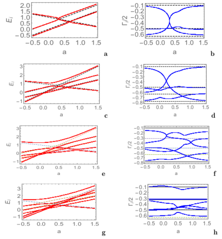
Figure 1: The eigenvalue trajectories ${\cal E}_{i}\equiv E_{i}+i/2\Gamma_{i}$ of a different number $N$ of states located in a certain energy window, $N=~{}3,~{}4,~{}5$ and 6. In all cases, the individual resonance states overlap. The parameters of the plots are: $e_{1}=1-a/2$; $e_{2}=a$; $e_{3}=1/2+a$; $e_{4}=2a$; $e_{5}=2a$; $e_{6}=a+1$; $\gamma_{1}/2=-.5$; $\gamma_{2}/2=-0.1$; $\gamma_{3}/2=-0.6335$; $\gamma_{4}/2=-0.323$; $\gamma_{5}/2=-0.31$; $\gamma_{6}/2=-0.5$; The off-diagonal elements of the coupling matrix are $\omega_{ij}=0.2$.

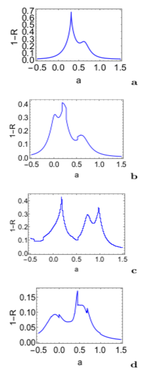
Figure 2: The eigenfunction trajectories corresponding to the eigenvalue trajectories of Fig. 1. The $R$ are averaged phase rigidities obtained by averaging over the individual phase rigidities $r_{i}$ of neighboring states in the considered energy interval. The 1-R averaged over the considered interval are  0.119819 for $N=3$;  0.122872 for $N=4$;  0.164372 for $N=5$;  0.0634185 for $N=6$.

In Fig. 1, the eigenvalue trajectories obtained from a calculation with respectively $N=3,~{}4,~{}5$ and $6$ states are shown. The differences of the results arise from the different degree of overlapping of the states in the different subfigures. The corresponding eigenfunction trajectories are shown in Fig. 2. The averaged phase rigidities $R$ are the individual phase rigidities $r_{i}$ of the states $i$ averaged over the number of neighboring states in the considered energy interval.

On the one hand, the value $R$ is an indicator for the difference between the description of the system by a non-Hermitian Hamiltonian and that by a Hermitian one. In other words when the value of $R$ is near to 1, the difference between the description of an open quantum system by a Hermitian and that by a non-Hermitian Hamiltonian is not remarkable. According to our results, this happens only when the number $N$ of states is really large, see Fig. 2.d.

On the other hand, the value $R$ contains also information on the role of nonlinear terms which are involved in the equations. As expected, $R$ decreases first with the number $N$ of states in the considered parameter region, see the caption of Fig. 2. For $N\to 6$, however, $R\to 1$ according to Fig. 2.d.

The results show a similar behavior of all eigenvalue and eigenfunction trajectories in the considered energy window. It is the behavior characteristic of interferences, and the EPs cannot be identified at large $N$. Here, hints to their existence even vanish. The interferences are caused by the individual contributions from all the resonance states at each point in the considered energy window. That means the individual resonance states contribute to the cross section not only in a restricted small parameter range near to an EP. They contribute rather to the cross section in a relatively large parameter range around the EPs, and the contributions of the different resonance states overlap (when the level density is sufficiently large). Such a behavior is, of course, described best by means of the different nonlinear contributions (caused by the individual EPs) to the cross section.

Most interesting are the results for $N=6$. Additionally to the results shown in Figs. 1 and 2, we performed calculations also for resonance states different from those in these figures, such that the results are of broader meaning. In all cases, the features typical of the eigenfunctions of a non-Hermitian operator vanish at large $N$. The phases of the eigenfunctions become rigid in the energy window considered, i.e. they behave like the phases of the eigenfunctions of a Hermitian operator. Correspondingly, the averaged value $R$ approaches the value $1$. Obviously, the system is described at high level density best by the Hermitian formalism with inclusion of nonlinear effects.

IV Conclusions

The numerical results represented in the two figures show very clearly that the nonlinearities arising from the EPs determine the behavior of realistic physical systems at high level density. It is therefore justified to replace the concept EP (defined at a certain point in the parameter space) by the synonym nonlinearity (defined in a much broader parameter range). Such a replacement corresponds to the real situation appearing in (small) open quantum systems at high level density.

References

- (1) I. Rotter, J. Phys. A 42, 153001 (2009)
- (2) I. Rotter and J.P. Bird, Rep. Prog. Phys. 78, 114001 (2015)
- (3) H. Friedrich and D. Wintgen, Phys. Rev. A 31, 3964 (1985)
- (4) H. Friedrich and D. Wintgen, Phys. Rev. A 32, 3231 (1985)
- (5) I. Rotter, Entropy 20, 441 (2018)
- (6) T. Kato, Perturbation Theory for Linear Operators, Springer, Berlin 1966
- (7) U. Gunther, I. Rotter and B.F. Samsonov, J. Phys. A 40, 8815 (2007)
- (8) H. Eleuch and I. Rotter, Phys. Rev. A 95, 022117 (2017)
- (9) In contrast to the definition that is used in, for example, nuclear physics, we define the complex energies before and after diagonalization of by and , respectively, with and for decaying states. This definition will be useful when discussing systems with gain (positive widths) and loss (negative widths).
- (10) Y.V. Fyodorov and D.V. Savin, Phys. Rev. Lett. 108, 184101 (2012)
- (11) J.B. Gros, U. Kuhl, O. Legrand, F. Mortessagne, E. Richalot, and D.V. Savin, Phys. Rev. Lett. 113, 224101 (2014)