Master Majorana neutrino mass parametrization

Abstract

After introducing a master formula for the Majorana neutrino mass matrix we present a master parametrization for the Yukawa matrices automatically in agreement with neutrino oscillation data. This parametrization can be used for any model that induces Majorana neutrino masses. The application of the master parametrization is also illustrated in an example model, with special focus on its lepton flavor violating phenomenology.

Introduction: The Standard Model (SM) of particle physics stands as one of the most successful physical theories ever built. However, despite its tremendous success, it cannot describe all particle physics phenomena. Neutrino oscillation experiments have firmly established that neutrinos have non-zero masses and mixings, hence demanding an extension of the SM that accounts for them.

Many neutrino mass models have been proposed. A short list, to quote only a few reviews and general classification papers, includes models with Dirac Ma:2016mwh ; CentellesChulia:2018gwr or Majorana neutrinos Ma:1998dn , with neutrino masses induced at tree-level or radiatively at 1-loop/2-loop Cai:2017jrq or 3-loop Cepedello:2018rfh , at low- Boucenna:2014zba or high-energy scales, and by operators of dimension 5 or higher dimensionalities Anamiati:2018cuq .

The goal of this letter is twofold. First, we will introduce a master formula that unifies all Majorana neutrino mass models, which can be regarded as particular cases of this general expression. And second, we will present a master parametrization for the Yukawa matrices appearing in this formula. The parametrization presented in this letter extends previous results in the literature Casas:2001sr and can be used for any model that induces Majorana neutrino masses.

The master formula: With full generality, a Majorana neutrino mass matrix can be written in the form

$$m=f\,\left(y_{1}^{T}\,M\,y_{2}+y_{2}^{T}\,M^{T}\,y_{1}\right)\,.$$ (1)

Here $m$ is the $3\times 3$ complex symmetric neutrino mass matrix, which can be diagonalized as

$$D_{m}=\text{diag}\left(m_{1},m_{2},m_{3}\right)=U^{T}\,m\,U\,,$$ (2)

with $U$ a $3\times 3$ unitary matrix ($U^{\dagger}U=UU^{\dagger}=\mathbb{I}_{3}$). The matrices $y_{1}$ and $y_{2}$ are general dimensionless $n_{1}\times 3$ and $n_{2}\times 3$ complex matrices, respectively, and $M$ is a $n_{1}\times n_{2}$ complex matrix with dimension of mass. Without loss of generality, we will assume $n_{1}\geq n_{2}$. We note that $m$ must contain at least two non-vanishing eigenvalues in order to explain neutrino oscillation data. Therefore, in the following we consider $r_{m}=\text{rank}(m)=2\,\text{or}\,3$.

Eq. (1) is a master formula valid for all Majorana neutrino mass models. This can be illustrated with several examples. The simplest one is based on the popular seesaw mechanism Minkowski:1977sc ; Yanagida:1979as ; Mohapatra:1979ia ; GellMann:1980vs ; Magg:1980ut ; Schechter:1980gr , in particular on the standard type-I seesaw with $3$ generations of right-handed neutrinos. The light neutrino mass matrix in this model is given by $m=-\langle H^{0}\rangle^{2}\,y^{T}M_{R}^{-1}y$, an expression that can be obtained with the master formula by taking $f=-1$, $y_{1}=y_{2}=y/\sqrt{2}$ and $M=\langle H^{0}\rangle^{2}\,M_{R}^{-1}$. Here $\langle H^{0}\rangle=v/\sqrt{2}$ is the SM Higgs vacuum expectation value (VEV) and $M_{R}$ the Majorana mass matrix for the right-handed neutrinos. Moreover, these matrices are all $3\times 3$ and hence $n_{1}=n_{2}=3$ in this model. The mass matrices of more complicated Majorana neutrino models can also be accommodated with the master formula. For instance, the inverse seesaw Mohapatra:1986bd would correspond to $M=\langle H^{0}\rangle^{2}\,(M_{R}^{T})^{-1}\mu M_{R}^{-1}$, with $\mu$ the small lepton number violating mass scale in this model, whereas the scotogenic model Ma:2006km , in which neutrino masses are induced at the 1-loop level, corresponds to $f=\lambda_{5}/(16\pi^{2})$ and $M=\langle H^{0}\rangle^{2}\,M_{R}^{-1}F_{\rm loop}$, with $\lambda_{5}$ the coupling of the quartic term $(H^{\dagger}\eta)^{2}$ involving the standard ($H$) and inert ($\eta$) scalar doublets, and $F_{\rm loop}$ a matrix of loop functions. In particular, models with $y_{1}\neq y_{2}$ can be described with the master formula, as shown below with the specific example of the BNT model Babu:2009aq .

The master parametrization: Our goal after introducing the master formula in Eq. (1) is to establish a parametrization of the $y_{1}$ and $y_{2}$ Yukawa matrices with three properties:

• General: valid for all models.

• Complete: containing all the degrees of freedom in the model.

• Programmable: easy to use in phenomenological analyses.

Matrix	Dimensions	Property	Real parameters
$X_{1}$	$(n_{2}-n)\times 3$	Absent if $n=n_{2}$	$6(n_{2}-n)$
$X_{2}$	$(n_{1}-n_{2})\times 3$	Absent if $n_{1}=n_{2}$	$6(n_{1}-n_{2})$
$X_{3}$	$(n_{2}-n)\times 3$	Absent if $n=n_{2}$	$6(n_{2}-n)$
$W$	$n\times r$		$r(2n-r)$
$T$	$r\times r$	Upper triangular with $(T)_{ii}>0$	$r^{2}$
$K$	$r\times r$	Antisymmetric	$r(r-1)$
$\bar{B}$	$(n-r)\times 3$	Absent if $n=r$	$6(n-r)$
$C_{1}$	$r\times 3$	Case-dependent	$0$ or $2$
$C_{2}$	$3\times 3$	Case-dependent	-

Table 1: Matrices containing free parameters in the master parametrization. Even though the matrix $C_{2}$ does not contain any free parameter, we include it in this list since its form depends on the values of $r_{m}$ and $r$.

We will call this parametrization of the Yukawa matrices the master parametrization. We now proceed to present it. The Yukawa matrices $y_{1}$ and $y_{2}$ can be generally parametrized as

$$y_{1} =\frac{1}{\sqrt{2\,f}}\,V_{1}^{\dagger}\,\left(\begin{array}[]{c}\Sigma^{-1/2}\,W\,A\\ X_{1}\\ X_{2}\end{array}\right)\,\bar{D}_{\sqrt{m}}\,U^{\dagger}\,,$$ (6)

$$y_{2} =\frac{1}{\sqrt{2\,f}}\,V_{2}^{\dagger}\,\left(\begin{array}[]{c}\Sigma^{-1/2}\,\widehat{W}^{\ast}\,\widehat{B}\\ X_{3}\end{array}\right)\,\bar{D}_{\sqrt{m}}\,U^{\dagger}\,.$$ (9)

Several matrices have been defined in the previous two expressions, where $\ast$ denotes the conjugate matrix. We have defined the matrix $\bar{D}_{\sqrt{m}}$ as diag$\left(\sqrt{m_{1}},\sqrt{m_{2}},\sqrt{m_{3}}\right)$ if $r_{m}=3$ or diag$\left(\sqrt{m_{1}},\sqrt{m_{2}},\sqrt{v}\right)$ if $r_{m}=2$. In fact, $v$ can be replaced in this definition by any non-vanishing reference mass scale since it is a dummy variable that drops out in the calculation of the neutrino mass matrix. A singular-value decomposition has been applied to the matrix $M$,

$$M=V_{1}^{T}\,\widehat{\Sigma}\,V_{2}\,,$$ (10)

where $\widehat{\Sigma}$ is a $n_{1}\times n_{2}$ matrix that can be written as

$$\widehat{\Sigma}=\left(\begin{array}[]{c}\begin{array}[]{cc}\Sigma&0\\ 0&0_{n_{2}-n}\end{array}\\ \hline\cr 0_{n_{1}-n_{2}}\end{array}\right)\,,$$ (11)

and $\Sigma=\text{diag}\left(\sigma_{1},\sigma_{2},\dots,\sigma_{n}\right)$ is a diagonal $n\times n$ matrix containing the positive and real singular values of $M$ ($\sigma_{i}>0$). Therefore, we define $n$ as the number of non-zero singular values of the matrix $M$. Since the total number of singular values of $M$ is $n_{2}$, it is clear that $n\leq n_{2}$. It is possible to have vanishing singular values which are specifically encoded in the zero square $(n_{2}-n)\times(n_{2}-n)$ matrix $0_{n_{2}-n}$. $V_{1}$ and $V_{2}$ are $n_{1}\times n_{1}$ and $n_{2}\times n_{2}$ unitary matrices and can be found by diagonalizing the square matrices $MM^{\dagger}$ and $M^{\dagger}M$, respectively. $X_{1}$, $X_{2}$ and $X_{3}$ are, respectively, $(n_{2}-n)\times 3$, $(n_{1}-n_{2})\times 3$ and $(n_{2}-n)\times 3$ arbitrary complex matrices with dimensions of mass^-1/2. $\widehat{W}$ is an $n\times n$ matrix defined as

$$\widehat{W}=\left(W\quad\bar{W}\right)\,,$$ (12)

where $W$ is an $n\times r$ complex matrix, with $r=\text{rank}(W)$, such that $W^{\dagger}W=W^{T}W^{*}=\mathbb{I}_{r}$, and $\bar{W}$ is an $n\times(n-r)$ complex matrix, built with vectors that complete those in $W$ to form an orthonormal basis of $\mathbb{C}^{n}$. Therefore, $\widehat{W}$ is a unitary complex $n\times n$ matrix. $A$ is an $r\times 3$ matrix, which can be written as

$$A=T\,C_{1}\,,$$ (13)

with $T$ an upper-triangular $r\times r$ invertible square matrix with positive real values in the diagonal, and $C_{1}$ is an $r\times 3$ matrix. $\widehat{B}$ is an $n\times 3$ complex matrix defined as

$$\widehat{B}=\left(\begin{array}[]{c}B\\ \bar{B}\\ \end{array}\right)\,,$$ (14)

with $\bar{B}$ an arbitrary $(n-r)\times 3$ complex matrix and $B$ an $r\times 3$ complex matrix given by

$$B\equiv B\left(T,K,C_{1},C_{2}\right)=\left(T^{T}\right)^{-1}\,\left[C_{1}\,C_{2}+K\,C_{1}\right]\,,$$ (15)

where we have introduced the antisymmetric $r\times r$ square matrix $K$ and the $3\times 3$ matrix $C_{2}$. The exact form of the matrices $C_{1}$ and $C_{2}$ depends on the values of $r_{m}$ and $r$. For $r_{m}=r=3$ these matrices take the form

$$C_{1}=\mathbb{I}_{3},\quad C_{2}=\mathbb{I}_{3}+K_{12}\,\frac{T_{13}}{T_{11}}\,\left(\begin{array}[]{ccc}0&0&0\\ 0&0&1\\ 0&-1&0\end{array}\right)\,,$$ (19)

while the expressions for other cases, as well as a rigorous mathematical proof of the master parametrization, will be given elsewhere future . We summarize the matrices that appear in the master parametrization and count their free parameters in Tab. 1.

Parameter counting: In order to guarantee that the master parametrization is complete, a detailed parameter counting must be performed. In full generality, one can write

$$\texttt{\#}_{\rm free}=\texttt{\#}_{y_{1}}+\texttt{\#}_{y_{2}}-\texttt{\#}_{\rm eqs}-\texttt{\#}_{\rm extra}=6(n_{1}+n_{2})-\texttt{\#}_{\rm eqs}-\texttt{\#}_{\rm extra}\,,$$ (20)

where $\texttt{\#}_{y_{1}}=2\cdot 3\cdot n_{1}$ and $\texttt{\#}_{y_{2}}=2\cdot 3\cdot n_{2}$ are the number of real degrees of freedom in $y_{1}$ and $y_{2}$, respectively, and $\texttt{\#}_{\rm eqs}$ is the number of independent (real) equations contained in Eq. (1). Since this matrix equation is symmetric, one would naively expect to have 6 complex equations, which would then translate into 12 real restrictions on the elements of $y_{1}$ and $y_{2}$. However, one can check by direct computation that for $r=1$ one of the complex equations is actually redundant and can be derived from the other five. Therefore,

$$\texttt{\#}_{\rm eqs}=\left\{\begin{array}[]{l}12\quad\text{for}\,r=3\,\text{or}\,2,\\ 10\quad\text{for}\,r=1.\end{array}\right.$$ (21)

Note that the case $r=1$ is allowed only because (1) contains two terms, each of which in principle can be of rank 1, as long as the rank of the sum of both terms is 2. Finally, $\texttt{\#}_{\rm extra}$ is the number of extra (real) restrictions imposed on $y_{1}$ and $y_{2}$. In the most common case of the standard type-I seesaw one has $\texttt{\#}_{\rm extra}=0$. However, scenarios with additional restrictions have $\texttt{\#}_{\rm extra}\neq 0$. The total number of free parameters $\texttt{\#}_{\rm free}$ must match the sum of the number of free parameters in each of the matrices appearing in the master parametrization of Eqs. (6) and (9). Therefore

$$\texttt{\#}_{\rm free} =\texttt{\#}_{X_{1}}+\texttt{\#}_{X_{2}}+\texttt{\#}_{X_{3}}+\texttt{\#}_{A}+\texttt{\#}_{W}+\texttt{\#}_{B}+\texttt{\#}_{\bar{B}}+\texttt{\#}_{C_{1}}$$

$$=\texttt{\#}_{X_{1}}+\texttt{\#}_{X_{2}}+\texttt{\#}_{X_{3}}+\texttt{\#}_{T}+\texttt{\#}_{W}+\texttt{\#}_{K}+\texttt{\#}_{\bar{B}}+\texttt{\#}_{C_{1}}\,.$$ (22)

In the previous expressions we have taken $\texttt{\#}_{\bar{W}}=0$ and assigned all the free parameters in the product $\bar{W}\,\bar{B}$ to $\bar{B}$. This is possible because these two matrices always appear in the combination $\bar{W}\,\bar{B}$ and, given that all the parameters contained in $\bar{B}$ are free, $\texttt{\#}_{\bar{W}\bar{B}}\equiv\texttt{\#}_{\bar{B}}$.

It proves convenient to discuss a particular example in order to understand the general parameter counting procedure. Let us consider $n_{1}=n_{2}=n=3$ and focus on a scenario with $(r_{m},r)=(3,3)$. In this case $\widehat{\Sigma}\equiv\Sigma$, $\texttt{\#}_{\rm eqs}=12$ and $\texttt{\#}_{\rm extra}=0$. Therefore, from Eq.(20), one finds $\texttt{\#}_{\rm free}^{(3,3)}=24$. Using now Eq. (22), one finds

$$\texttt{\#}_{\rm free}^{(3,3)}=24=\texttt{\#}_{W}^{(3,3)}+\texttt{\#}_{A}^{(3,3)}+\texttt{\#}_{B}^{(3,3)}+\texttt{\#}_{C_{1}}^{(3,3)}=15+\texttt{\#}_{W}^{(3,3)}\,,$$ (23)

where $\texttt{\#}_{W}^{(3,3)}=9$ is the number of real free parameters in the matrix $W$ in the $(3,3)$ case. We point out that $\texttt{\#}_{W}^{(3,3)}=9$ also follows from the fact that $W$ is a unitary $3\times 3$ matrix, which makes a good consistency check of the parameter counting we just performed. In addition, we note that $\texttt{\#}_{A}^{(3,3)}=9$ and $\texttt{\#}_{B}^{(3,3)}=6$.

The Casas-Ibarra limit: One must finally compare the master parametrization to previously known parametrizations in the literature. In particular, let us compare to the Casas-Ibarra parametrization Casas:2001sr . As already explained above, the type-I seesaw corresponds to $y_{1}=y_{2}=y/\sqrt{2}$, $n_{1}=n_{2}=n=r=3$, $f=-1$ and $M=\langle H^{0}\rangle^{2}M_{R}^{-1}$. Furthermore, in this model the symmetric matrix $M$ can be diagonalized by a single matrix, $V_{1}=V_{2}$, which can be taken to be the identity if the right-handed neutrinos are in their mass basis, and the matrices $X_{1,2,3}$, $\overline{W}$ and $\overline{B}$ drop from all the expressions. Finally, imposing $y_{1}=y_{2}$ is equivalent to $W^{T}WA=B$. Solving this matrix equation leads to $B=\left(A^{T}\right)^{-1}$ and allows one to define $R=W\,A$, with $R$ a general $3\times 3$ orthogonal matrix. Replacing all these ingredients into Eqs. (6) and (9) one finds

$$y=\sqrt{2}\,y_{1}=\sqrt{2}\,y_{2}=i\,\Sigma^{-1/2}\,R\,D_{\sqrt{m}}\,U^{\dagger}\,,$$ (24)

which is nothing but the Casas-Ibarra parametrization for the type-I seesaw Yukawa matrices. We note that $R$ can be identified with the usual Casas-Ibarra matrix Casas:2001sr . Imposing $y_{1}=y_{2}$ leads to $18\,(=9\cdot 2)$ real constraints, this is, $\texttt{\#}_{\rm extra}=18$. Therefore, direct application of the general counting formula in Eq. (20) leads to $\texttt{\#}_{\rm free}=6$. These are the free real parameters contained in $R$ which can be parametrized by means of $3$ complex angles. We conclude that the Casas-Ibarra parametrization can be regarded as a particular case of the general master parametrization.

An application: The full power of the master parametrization is better illustrated with an application to the BNT model Babu:2009aq . In addition to the SM particles, the model contains three copies of the vector-like fermions $\psi_{L,R}$ transforming as $({\bf 1},{\bf 3},-1)$ under the SM gauge group and an exotic scalar $\Phi$ transforming as $({\bf 1},{\bf 4},3/2)$. The quantum numbers of the new particles in the BNT model are given in Table 2.

	generations	$\mathrm{SU(3)}_{c}$	$\mathrm{SU(2)}_{L}$	$\mathrm{U(1)}_{Y}$
$\Phi$	1	${\bf 1}$	${\bf 4}$	$3/2$
$\psi_{L,R}$	3	${\bf 1}$	${\bf 3}$	$-1$

Table 2: New particles in the BNT model.

The Lagrangian of the model contains the following pieces relevant for neutrino mass generation

$$-\mathcal{L} \supset y_{\psi}\,\overline{L}\,H\,\psi_{R}+y_{\bar{\psi}}\,\overline{L^{c}}\,\Phi\,\psi_{L}+M_{\psi}\overline{\psi}\,\psi+\mathrm{h.c.}\,,$$ (25)

where we have omitted $\mathrm{SU(2)_{L}}$ and flavor indices to simplify the notation. The scalar potential of the model is given by

$$\mathcal{V} =M_{H}^{2}|H|^{2}+M_{\Phi}^{2}|\Phi|^{2}+\frac{1}{2}\lambda_{1}\,|H|^{4}+\frac{1}{2}\lambda_{2}\,|\Phi|^{4}$$

$$+\lambda_{3}\,\left(|H|^{2}|\Phi|^{2}\right)_{\bf 1}+\lambda_{4}\,\left(|H|^{2}|\Phi|^{2}\right)_{\bf 3}+\lambda_{\Phi}\,\left[H^{3}\,\Phi^{\dagger}+\mathrm{h.c.}\right]\,.$$ (26)

Here $H$ is the SM Higgs doublet. We note that there are two possible $\mathrm{SU(2)_{L}}$ contractions of $|H|^{2}|\Phi|^{2}$, corresponding to the $\lambda_{3}$ and $\lambda_{4}$ quartic terms. All the couplings in the scalar potential must be real, with the exception of $\lambda_{\Phi}$, which can be complex. The introduction of $\lambda_{\Phi}\neq 0$ precludes the introduction of a non-vanishing lepton number for $\Phi$. In fact, one can easily see that lepton number is broken in two units in the BNT model. Furthermore, this term induces a non-zero VEV for the neutral component of $\Phi$, $\Phi^{0}$, which is given by

$$\langle\Phi^{0}\rangle=\frac{v_{\Phi}}{\sqrt{2}}=\frac{\lambda_{\Phi}v^{3}}{2\sqrt{2}M_{\Phi}^{2}}\,.$$ (27)

In the BNT model, neutrino masses are generated at dimension 7 as shown in Fig. 1. The resulting expression for the neutrino mass matrix is

$$m=\frac{\lambda_{\Phi}v^{4}}{4M_{\Phi}^{2}}\,\left[y_{\psi}^{T}\,M_{\psi}^{-1}\,y_{\bar{\psi}}+y_{\bar{\psi}}^{T}\,(M_{\psi}^{-1})^{T}\,y_{\psi}\right]\,.$$ (28)

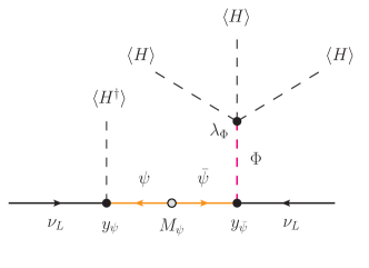
Figure 1: Neutrino mass generation in the BNT model.

The usual Casas-Ibarra parametrization cannot be applied in this model since one has two independent $y_{1}=y_{\psi}$ and $y_{2}=y_{\bar{\psi}}$ Yukawa matrices. Therefore, in order to guarantee that the parameters measured in neutrino oscillation experiments are correctly reproduced one must make use of the master parametrization. In order to apply the master parametrization we must first identify the different pieces taking part of the neutrino mass expression in the BNT model, Eq. (28). By direct comparison to the master formula in Eq. (1) we identify

$$f=\frac{\lambda_{\Phi}v^{2}}{2M_{\Phi}^{2}}\,,\quad M=\frac{v^{2}}{2}\,M_{\psi}^{-1}\,.$$ (29)

Furthermore, in this model $y_{1}$, $y_{2}$ and $M$ are $3\times 3$ matrices and then $n_{1}=n_{2}=3$. One also has $3$ non-vanishing singular values in $M$ and therefore $n=3$ and $\widehat{\Sigma}\equiv\Sigma$. Finally, taking $r=r_{m}=3$, the matrices $X_{1,2,3}$ and $\bar{B}$ are absent, while $C_{1}$ and $C_{2}$ are given in Eq. (19).

The application of the master parametrization is now straightforward. In the numerical scans that follow, the values of the neutrino oscillation parameters from the global fit deSalas:2017kay are imposed, thus guaranteeing the consistency with oscillation experiments. We have implemented the model in SARAH Staub:2013tta and obtained numerical results with the help of SPheno Porod:2011nf . In the following we concentrate on the lepton flavor violating (LFV) phenomenology of the model. The LFV observables have been computed with FlavorKit Porod:2014xia . Some selected results on the LFV observable Br$(\mu\to e\gamma)$ are shown in Figs. 2 and 3. When running a numerical scan of the BNT model, one can assume specific simple forms for the matrices that appear in the master parametrization (such as $T=\mathbb{I}$ or $K=0$) or cover more general parameter regions. Fig. 2 shows the results of a random scan with/without using the freedom in the matrices $T$ and $K$ as a function of $v_{\Phi}$, while Fig. 3 shows a contour plot in the plane [$T_{11},T_{12}$]. Both examples serve to demonstrate that it is important to scan over all allowed degrees of freedom in order to obtain a general result.

Figure 2: Example points for Br$(\mu\to e\gamma)$ in the BNT model as a function of the quadruplet VEV $v_{\Phi}$. This figure has been obtained by allowing the neutrino oscillation parameters to vary within the 3 $\sigma$ ranges determined by the global fit deSalas:2017kay , assuming normal hierarchy, $M_{\Psi}$ randomly taken in the interval $[0.5,2]$ TeV and $W=\mathbb{I}$. The purple points correspond to a scan in which the entries of the matrices $T$ and $K$ are randomly taken in the following ranges: $T_{ii}\in[0,2]$ and $K_{ij}$, $T_{ij}$ (with $i\neq j$) $\in[-1,1]$. The black points in the foreground correspond to a simplified scan with $T=\mathbb{I}$ and $K=0$.

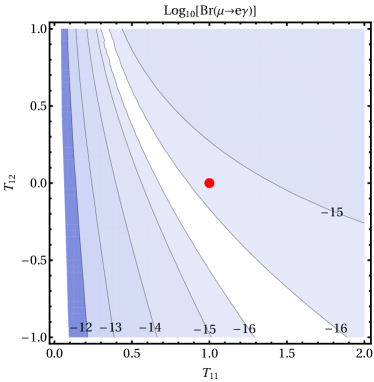
Figure 3: Example contours for Br$(\mu\to e\gamma)$ in the $(T_{11},T_{12})$ plane for the BNT model. Neutrino oscillation parameters are taken at their best fit points according to deSalas:2017kay , while $M_{\Psi}=0.5$ TeV and $v_{\Phi}=10$ KeV are fixed. All entries in the matrices $W$, $T$ and $K$ are taken to be trivial ($W=T=\mathbb{I}$ and $K=0$), except for $T_{11}$ and $T_{12}$, which are left as free parameters. The point in the middle of the plot [$T_{11}=1,T_{12}=0$] corresponds to a simplified scenario with $T=\mathbb{I}$.

Final discussion: The master parametrization allows one to explore the parameter space of any Majorana neutrino mass model in a complete way, while fixing at the same time the parameters to be in agreement with all neutrino data. The master parametrization is easy to program, thus making parameter space exploration more direct than ever. The master parametrization may also provide analytical insight on some scenarios.

The application of the master parametrization is straightforward. First, one must use the information from neutrino oscillation experiments to fix the light neutrino masses and leptonic mixing angles appearing in $\bar{D}_{\sqrt{m}}$ and $U$, respectively. Then, by comparing the expression for the mass matrix of the light neutrinos in the model under consideration with the general master formula in Eq. (1) one can easily identify the global factor $f$, the Yukawa matrices $y_{1}$ and $y_{2}$ as well as the matrix $M$. The latter can be singular-value decomposed to determine $\Sigma$, $V_{1}$ and $V_{2}$, while the Yukawa matrices $y_{1}$ and $y_{2}$ are expressed in terms of a set of matrices ($\widehat{W}$, $X_{1,2,3}$, $\bar{B}$, $T$, $K$ and $C_{1,2}$) by means of the master parametrization in Eqs. (6) and (9). In a numerical analysis one can simply randomly scan over the free parameters contained in these matrices to completely explore the parameter space of a given model.

In closing, we should also point out some potential limitation of our approach: In exceptional cases, the master parametrization may become either unnecessary, not direct or impractical. Exceptional cases are simply those for which $y_{1}$ and $y_{2}$ are not completely free parameters. A first category of exceptional models is given by those with $y_{1}=y_{2}=\mathbb{I}$, such as in type-II seesaw. However, this example of an unnecessary case can also trivially be solved. More involved situations are found in models with symmetric Anamiati:2016uxp or antisymmetric Zee:1980ai ; Cheng:1980qt ; Zee:1985id ; Babu:1988ki Yukawa matrices, or models in which the Yukawa matrices have specific textures imposed by flavor symmetries. For such cases the master parametrization may be applicable only with additional constraints or become even impractical. We plan to return to a more detailed discussion of these cases in a future publication future .

References

- (1) E. Ma and O. Popov, Phys. Lett. B 764 (2017) 142 doi:10.1016/j.physletb.2016.11.027 [arXiv:1609.02538 [hep-ph]].
- (2) S. Centelles Chuliá, R. Srivastava and J. W. F. Valle, Phys. Lett. B 781 (2018) 122 doi:10.1016/j.physletb.2018.03.046 [arXiv:1802.05722 [hep-ph]].
- (3) E. Ma, Phys. Rev. Lett. 81 (1998) 1171 doi:10.1103/PhysRevLett.81.1171 [hep-ph/9805219].
- (4) Y. Cai, J. Herrero-García, M. A. Schmidt, A. Vicente and R. R. Volkas, Front. in Phys. 5 (2017) 63 doi:10.3389/fphy.2017.00063 [arXiv:1706.08524 [hep-ph]].
- (5) R. Cepedello, R. M. Fonseca and M. Hirsch, JHEP 1810, 197 (2018) doi:10.1007/JHEP10(2018)197 [arXiv:1807.00629 [hep-ph]].
- (6) S. M. Boucenna, S. Morisi and J. W. F. Valle, Adv. High Energy Phys. 2014 (2014) 831598 doi:10.1155/2014/831598 [arXiv:1404.3751 [hep-ph]].
- (7) G. Anamiati, O. Castillo-Felisola, R. M. Fonseca, J. C. Helo and M. Hirsch, arXiv:1806.07264 [hep-ph].
- (8) J. A. Casas and A. Ibarra, Nucl. Phys. B 618 (2001) 171 doi:10.1016/S0550-3213(01)00475-8 [hep-ph/0103065].
- (9) P. Minkowski, Phys. Lett. 67B (1977) 421. doi:10.1016/0370-2693(77)90435-X
- (10) T. Yanagida, Conf. Proc. C 7902131 (1979) 95.
- (11) R. N. Mohapatra and G. Senjanovic, Phys. Rev. Lett. 44 (1980) 912. doi:10.1103/PhysRevLett.44.912
- (12) M. Gell-Mann, P. Ramond and R. Slansky, Conf. Proc. C 790927 (1979) 315 [arXiv:1306.4669 [hep-th]].
- (13) M. Magg and C. Wetterich, Phys. Lett. 94B (1980) 61. doi:10.1016/0370-2693(80)90825-4
- (14) J. Schechter and J. W. F. Valle, Phys. Rev. D 22 (1980) 2227. doi:10.1103/PhysRevD.22.2227
- (15) R. N. Mohapatra and J. W. F. Valle, Phys. Rev. D 34 (1986) 1642. doi:10.1103/PhysRevD.34.1642
- (16) E. Ma, Phys. Rev. D 73 (2006) 077301 doi:10.1103/PhysRevD.73.077301 [hep-ph/0601225].
- (17) K. S. Babu, S. Nandi and Z. Tavartkiladze, Phys. Rev. D 80 (2009) 071702 doi:10.1103/PhysRevD.80.071702 [arXiv:0905.2710 [hep-ph]].
- (18) I. Cordero-Carrión, M. Hirsch and A. Vicente, to appear.
- (19) P. F. de Salas, D. V. Forero, C. A. Ternes, M. Tortola and J. W. F. Valle, Phys. Lett. B 782 (2018) 633 doi:10.1016/j.physletb.2018.06.019 [arXiv:1708.01186 [hep-ph]].
- (20) F. Staub, Comput. Phys. Commun. 185 (2014) 1773 doi:10.1016/j.cpc.2014.02.018 [arXiv:1309.7223 [hep-ph]].
- (21) W. Porod and F. Staub, Comput. Phys. Commun. 183 (2012) 2458 doi:10.1016/j.cpc.2012.05.021 [arXiv:1104.1573 [hep-ph]].
- (22) W. Porod, F. Staub and A. Vicente, Eur. Phys. J. C 74 (2014) no.8, 2992 doi:10.1140/epjc/s10052-014-2992-2 [arXiv:1405.1434 [hep-ph]].
- (23) G. Anamiati, M. Hirsch and E. Nardi, JHEP 1610 (2016) 010 doi:10.1007/JHEP10(2016)010 [arXiv:1607.05641 [hep-ph]].
- (24) A. Zee, Phys. Lett. 93B (1980) 389 Erratum: [Phys. Lett. 95B (1980) 461]. doi:10.1016/0370-2693(80)90349-4, 10.1016/0370-2693(80)90193-8
- (25) T. P. Cheng and L. F. Li, Phys. Rev. D 22 (1980) 2860. doi:10.1103/PhysRevD.22.2860
- (26) A. Zee, Nucl. Phys. B 264 (1986) 99. doi:10.1016/0550-3213(86)90475-X
- (27) K. S. Babu, Phys. Lett. B 203 (1988) 132. doi:10.1016/0370-2693(88)91584-5