Simulating dynamically assisted production of Dirac pairs
in gapped graphene monolayers

Abstract

In a vicinity of the Fermi surface, graphene layers with bandgaps allow for closely simulating the vacuum of quantum electrodynamics and, thus, its yet unverified strong-field phenomenology with accessible field strengths. This striking feature is exploited to investigate a plausible materialization of dynamically assisted pair production through the analog production of light but massive pairs of Dirac quasiparticles. The process is considered in a field configuration combining a weak high-frequency electric mode and a strong low-frequency electric field oscillating in time. Its theoretical study is carried out from a quantum kinetic approach, similar to the one governing the spontaneous production of pairs in QED. We show that the presence of the weak assisting mode can strongly increase the number of produced massive Dirac pairs as compared with a setup driven by the strong field only. The efficiency of the process is contrasted, moreover, with the case of gapless graphene to highlight the role played by the quasiparticle mass.

I Introduction

Perceiving the vacuum as a region in which quantum fluctuations of all realizable fields in nature occur has always been accompanied by the intriguing possibility of their materialization into real particles at the expense of the vacuum instability. Among field theories describing the fundamental interactions, quantum electrodynamics (QED) provides the most accessible scenario in which this phenomenon could be realized. There, the spontaneous production of fermions is predicted to occur in form of electron-positron pairs if an electric-like background [$E^{2}-B^{2}>0$] polarizes the quantum vacuum. The simplest configuration allowing for the pair production (PP) process – commonly known as the Schwinger mechanism – requires just a constant electric field [$B=0,\;E=\rm const$]. In such a situation, the associated PP rate $\mathcal{R}\sim\exp[-\pi m^{2}c^{3}/(e\hbar E)]$ manifests an essential singularity in the coupling strength $e$ indicating the nonperturbative nature of this striking strong field phenomenon Sauter:1931 ; Heisenberg:1935 ; Schwinger:1951nm . That the Schwinger mechanism has so far eluded any detection agrees with the exponential suppression that $\mathcal{R}$ undergoes, because – by now – it is impossible to generate macroscopically extended electric fields with amplitude $E$ comparable to the critical scale in QED, $E_{\rm cr}=m^{2}c^{3}/(e\hbar)\sim 10^{16}\ \rm V/cm$.

Due to continuous progress toward high-power lasers facilities, the possibility of observing the (dynamical) Schwinger mechanism in tightly focused pulses is currently receiving considerable attention. Envisaged multi-petawatt facilities such as the Extreme Light Infrastructure (ELI) ELI and the Exawatt Center for Extreme Light Studies (XCELS) xcels are expected to achieve peak field strengths of the order of $\sim 10^{-2}E_{\rm cr}$, which will bring the PP process closer to experimental accessibility. Motivated by these prospects, theoreticians have studied special configurations of laser fields that might help to attain a detectable PP signal (see Refs. Hebenstreit:2014lra ; Bulanov2010 and references therein). In particular, various proposals have been put forward to mitigate the exponential suppression of the Schwinger pair creation rate dgs2008 ; dgs2009 ; Orthaber2011 ; Grobe2012 ; Akal:2014eua ; Otto:2014ssa ; Linder:2015vta ; Panferov:2015yda ; torgrimsson2016 ; Akal:2017em . Indeed, compelling theoretical evidences indicate a significant enhancement of the PP rate $\mathcal{R}\sim\exp[-\kappa E_{\rm cr}/E]$ with $0<\kappa\ll 1$, when the strong field configuration is assisted by a fast-oscillating laser beam of weaker intensity. In a physically intuitive picture, this enhancement in $\mathcal{R}$ is caused by the absorption of a photon from the fast-oscillating field, this way reducing effectively the width of the barrier that an electron has to tunnel from negative to positive Dirac continuum.

Although promising, this so-called dynamically assisted Schwinger mechanism still awaits a proof-of-principle test, and even with the envisaged fields in operation, it is likely that its experimental verification remains a very challenging task. A complementary route for probing the vacuum instability assisted by an additional fast-oscillating wave is to look for a QED-like vacuum in which the mentioned process becomes manifest at much lower energies and field strengths. In this sense, graphene monolayers designed with a bandgap $\Delta\varepsilon\lesssim 0.3\ \rm eV$ Substrate1 ; Substrate2 ; basov ; Varykhalov constitute an ideal scenario. Indeed, recent measurements of optical radiation emitted from regular graphene layers [$\Delta\varepsilon=0$] irradiated by ultrashort terahertz pulses, provide strong evidence about the interband transition of electrons in the field of the THz pulse. The radiation is presumably caused by the recombinations of electron-hole pairs created via the Schwinger mechanism Oladyshkin . See also Refs. Lui ; Tani .

The suitability of bandgapped – or semiconductor – graphene layers can be understood as a direct consequence of the quasiparticle mass $\mathpzc{m}=\Delta\varepsilon/(2\mathpzc{v}_{f}^{2})\lesssim 10\ \mathrm{keV}/c^{2}$ [with $\mathpzc{v}_{f}\approx c/300$ the Fermi velocity] and the relativistic-like dispersion relation $\mathpzc{w}_{\boldsymbol{p}}=(\boldsymbol{p}^{2}\mathpzc{v}_{f}^{2}+\mathpzc{m}^{2}\mathpzc{v}_{f}^{4})^{\nicefrac{{1}}{{2}}}$ that Dirac fermions exhibit when their energies are nearby the Fermi surface, i.e. close to any of the two inequivalent Dirac points $\boldsymbol{K}_{\pm}$ in the reciprocal lattice Wallace . Indeed, within the nearest-neighbours tight-binding model these two properties allow us to closely simulate the matter sector of QED, and thus, its quantum vacuum. Likewise, the electron-positron PP process finds an analogous phenomenon: the field-induced creation of quasiparticle-hole pairs from valence to conduction band. Recently, the similarity has been stressed further by noticing that the associated PP rate in the vicinity of $\boldsymbol{K}_{\pm}$ closely resembles the exponential dependence $\mathcal{R}_{\mathpzc{g}}\sim\exp[-\pi\mathpzc{m}^{2}\mathpzc{v}_{f}^{3}/(e\hbar E)]$ found for the Schwinger mechanism Akal:2016stu . The feasibility for materializing relativistic-like tunneling in semiconductors has also been investigated in Ref. Linder:2015fba . As in QED, critical field strengths can be associated with these materials. For instance, in graphene varieties with band gaps this one $E_{\mathpzc{g}}=\mathpzc{m}^{2}\mathpzc{v}_{f}^{3}/(e\hbar)\lesssim 10^{5}\ \rm V/cm$ is set by the exponent of $\mathcal{R}_{\mathpzc{g}}$. However, in contrast to $E_{\mathrm{cr}}$, the latter can be easily overpassed with present-day laser technology, without damaging the material. This feature offers a genuine opportunity for a well-controllable materialization of both the Schwinger mechanism and its dynamically assisted version through the described solid-state analog.

Here, we investigate the production of quasiparticle-hole pairs in an external field configuration involving a fast-oscillating electric mode of weak intensity superposed on a strong, low-frequency electric field oscillating in time. Our study is carried out from a quantum kinetic approach, similar to the one governing the spontaneous PP process in QED. Our outcomes reveal that the number of created massive quasiparticles in this assisted setup can be strongly enhanced by the presence of the high-frequency mode. In particular, by exploiting the laser repetition rate in our bifrequent setup, the number of pairs can become comparable to the single-shot outcome resulting from a scenario in which the high-frequency wave is not present and the Dirac fermions are massless instead. The mentioned aspects are exposed in two sections. In Sec. II, we set the theoretical framework on which our study relies. Likewise, some important features of the production of electron-hole pairs in bandgapped graphene are analyzed in connection with transport theory. The numerical results are presented in Sec. III, where in parallel, the role of the resonant effects arising in the single-particle distribution function is discussed. Also the density of pairs yielded in the assisted field configuration is shown in this section. Further comments and remarks are given in the conclusions.

II Quantum kinetic approach

Let us briefly precise some general features linked to the spontaneous production of electron-hole pairs in graphene layers. Previous studies on this phenomenon have been carried out Allor:2007ei ; Mostepanenko ; Avetissian ; Fillion-Gourdeau:2015dga ; Fillion-Gourdeau:2016izx in connection with the absence of a gap $\Delta\varepsilon=0$ that the regular synthesization of graphene manifests GrExp1 ; GrExp2 ; GrExp3 . Such a characteristic constitutes, however, a drawback when thinking of materializing the dynamically-assisted PP process via the graphene analogue because the exponential suppression of the corresponding rate is removed fully. As this behavior is essential for judging both the plausible PP enhancement as well as the nonperturbative character of this phenomenon, we will suppose that the charge carriers can acquire a tiny mass $\mathpzc{m}=\Delta\varepsilon/2\mathpzc{v}_{f}^{2}$ corresponding to a gap $\Delta\varepsilon\sim 0.1\;\rm eV$ [$\lambda=2\pi/(\mathpzc{m}\mathpzc{v}_{f})\sim 0.1\ \rm nm$], which can originate from the epitaxial growth of graphene on SiC substrate Substrate1 ; Substrate2 , for instance. We emphasize that, in addition to this techniques, there exist a variety of well-known forms to induce gaps in the band structure of graphene. They include elastic strain basov or Rashba spin splittings on magnetic substrates Varykhalov .

From now on the external electric field $\boldsymbol{E}(t)=-\partial\boldsymbol{\mathpzc{A}}(t)/(c\partial t)$ [$\mathpzc{A}_{0}(t)=0$] is supposed spatially homogeneous but time dependent with

$$\boldsymbol{\mathpzc A}(t)= -\mathscr{F}(\phi)\left[\frac{cE_{s}}{\Omega}\sin(\phi)+\frac{cE_{w}}{\omega}\sin(\eta\phi)\right]\boldsymbol{n}.$$ (1)

Here $\Omega$ and $E_{s}$ are the respective frequency and the electric field amplitude of the strong field, whereas $\omega$ and $E_{w}$ correspond to the frequency and the field strength of the perturbative fast-oscillating wave. The parameters contained within the trigonometric functions are $\phi=\Omega t$ and $\eta=\omega/\Omega$. Besides, $\boldsymbol{n}^{T}=(0,1,0)$ defines the polarization direction of the field which we assume – hereafter – embedded in the plane defined by the graphene sheet, i.e. at $z=0$. In Eq. (1) the envelope function is chosen with $\sin^{2}$-ramping and de-ramping intervals, whereas a plateau region of constant field intensity is taken in between:

$$\begin{split}\mathscr{F}(\phi)&=\sin^{2}\left(\phi/2\right)\left[\Theta(\pi-\phi)\Theta(\phi)+\Theta(2\pi N-\phi)\right.\\ &\times\left.\Theta(\phi-2\pi\mathpzc{K})\right]+\Theta(\phi-\pi)\Theta(2\pi\mathpzc{K}-\phi),\end{split}$$ (2)

where $N=N_{\mathrm{plateau}}+1$, $\mathpzc{K}=N-\frac{1}{2}$ and $\Theta(x)$ denotes the unit step function: $\Theta(x)=1$ at $x\geqslant 0$, $\Theta(x)=0$ at $x<0$. Here $N_{\mathrm{plateau}}$ counts for the number of cycles within the region where $\mathscr{F}(\phi)=1$. Observe that Eq. (1) and (2) guarantee the starting of the oscillating electric field with zero-amplitude at $t=0$.

There exist various ways of generating a field of this nature. A first option could be a head-on collision of two pairs of linearly polarized laser pulses sharing two frequencies, the same polarization directions and which propagate perpendicularly to the graphene sheet. A second option can be envisaged by combining the field generated by a capacitor with ac voltage and the one generated by the collision of two counterpropagating monochromatic laser waves which, as in the previous setup, impinge perpendicularly to the layer. Observe that, to fit with our theoretical treatment, the field directions of both time dependent electric components have to coincide. The described scenarios do not provide a homogeneous electric field; those resulting from the wave collisions depend on their direction of propagation. However, because of the chosen geometry, no essential effect due to the spatial inhomogeneity along the direction of propagation is expected. Clearly, the field generated by the laser waves also has a transverse finite extension characterized by the waist size $w_{0}$, and so it is inhomogeneous in the $(x,y)-$plane. We remark that no impact due to this transverse focusing is expected either as long as $w_{0}$ turns out to be much larger than the length of the graphene layer, which we take here of the order of $\ell\sim\mathcal{O}(10)\;\rm\mu m$. Clearly, the counterpropagation of the electric-field-generating plane-waves could take place along the graphene sheet rather than perpendicular to it. If this is the case, the homogeneous electric field approximation requires the involved laser wavelengths $\lambda_{s,w}$ to exceed significantly the typical formation length of the PP process $\mathpzc{l}_{\mathrm{pair}}\sim\delta/|eE_{s}|$ with $\delta=\Delta\varepsilon-\omega$ DiPiazza:2009py ; Jansen2013 .

From the theory prospect, quantum kinetic theory constitutes an appropriate approach for investigating the production of electron-hole pairs in graphene. In contrast to perturbative processes in unstable vacuum–described by Feynman diagrams Gitman ; Fradkin –the dynamical information of the pure PP process can be comprised in the single-particle distribution function $W_{\mathpzc{g}}(\boldsymbol{p},t)$ of electrons and holes to which the degrees of freedom in the external field are relaxed at asymptotically large times [$t\to\pm\infty$], i.e., when the electric field is switched off $\boldsymbol{E}(\pm\infty)\to 0$. Whenever the momentum of the massive quasiparticles $\boldsymbol{p}$, relative to $\boldsymbol{K}_{\pm}$ satisfies the condition $|\boldsymbol{p}|\ \ll|\boldsymbol{K}_{\pm}|=\frac{4\pi}{3\sqrt{3}a_{0}}$ with $a_{0}=0.142\ \rm nm$ basov , the time evolution of this quantity is dictated by a quantum kinetic equation Akal:2016stu :

$$\dot{W}_{\mathpzc{g}}(\boldsymbol{p},t)=Q(\boldsymbol{p},t)\int_{-\infty}^{t}d\tilde{t}\;Q(\boldsymbol{p},\tilde{t})\left[\frac{1}{2}-W_{\mathpzc{g}}(\boldsymbol{p},\tilde{t})\right]$$

$$\qquad\quad\qquad\times\cos\left[2\int_{\tilde{t}}^{t}dt^{\prime}\ \mathpzc{w}_{\boldsymbol{p}}(t^{\prime})\right].$$ (3)

Here, the vacuum initial condition $W_{\mathpzc{g}}(\boldsymbol{p},-\infty)=0$ is assumed. This formula is characterized by the function $Q(\boldsymbol{p},t)\equiv eE(t)\mathpzc{v}_{f}\epsilon_{\perp}/\mathpzc{w}_{\boldsymbol{p}}^{2}(t)$, which depends on the transverse energy of the Dirac fermions $\epsilon_{\perp}=\sqrt{\mathpzc{m}^{2}\mathpzc{v}_{f}^{4}+p_{x}^{\,2}\mathpzc{v}_{f}^{2}}$ and their respective total energy squared $\mathpzc{w}^{2}_{\boldsymbol{p}}(t)=\epsilon_{\perp}^{2}+[p_{y}-e\mathpzc{A}(t)/c]^{2}\mathpzc{v}_{f}^{2}$ of a Dirac quasiparticle. As no dependence on temperature is manifested in Eq. (II), any prediction resulting from it must be understood within the zero temperature limit. We remark that, at asymptotically earlier times $t\to-\infty$ for which both $\mathpzc{A}(t),\;E(t)\to 0$, the system is assumed to meet equilibrium conditions. In this limit the total energy of a Dirac quasiparticle $\mathpzc{w}_{\boldsymbol{p}}(t)\to\sqrt{\boldsymbol{p}^{2}\mathpzc{v}_{f}^{2}+\mathpzc{m}^{2}\mathpzc{v}_{f}^{2}}$ has to be understood relative to the Fermi-level:

$$\varepsilon_{\mathrm{F}}=\mathpzc{mv}_{f}^{2}\left[\sqrt{\frac{\mathpzc{N}_{\;\mathrm{in}}}{\mathpzc{N}_{\;0}}+1}-1\right].$$ (4)

Here $\mathpzc{N}_{\;\mathrm{in}}$ denotes the initial density of Dirac fermions, whereas the constant value $\mathpzc{N}_{\;0}=g_{s}g_{v}\mathpzc{m}^{2}\mathpzc{v}_{f}^{2}/(4\pi)$ depends on the respective “spin” ($g_{s}=2$) and valley ($g_{v}=2$) degeneracy factors. For $\mathpzc{m}=11.7\;\mathrm{keV}/c^{2}$, corresponding to a bandgap $\Delta\varepsilon=0.26\;\rm eV$, $\mathpzc{N}_{\;0}\approx 1.26\times 10^{12}\;\rm cm^{-2}$. Observe that, in the limit $\mathpzc{N}_{\mathrm{in}}\gg\mathpzc{N}_{\;0}$, the Fermi energy reduces to the expression known for gapless graphene monolayers: $\varepsilon_{\mathrm{F}}\approx(\pi\mathpzc{v}_{f}^{2}\mathpzc{N}_{\;\mathrm{in}})^{\nicefrac{{1}}{{2}}}$.

Despite its compactness, the consequences embedded in Eq. (II) are often facilitated via equivalent systems of ordinary differential equations. Here we utilize one combining two equations in which the Bogoliubov coefficients $f(\boldsymbol{p},t)$ and $g(\boldsymbol{p},t)$ appear explicitly Akal:2014eua ; Akal:2016stu :

$$\begin{split}&i\dot{f}(\boldsymbol{p},t)=\mathpzc{a}_{\boldsymbol{p}}(t)f(\boldsymbol{p},t)+\mathpzc{b}_{\boldsymbol{p}}(t)g(\boldsymbol{p},t),\\ &i\dot{g}(\boldsymbol{p},t)=\mathpzc{b}^{*}_{\boldsymbol{p}}(t)f(\boldsymbol{p},t)-\mathpzc{a}_{\boldsymbol{p}}(t)g(\boldsymbol{p},t).\end{split}$$ (5)

In this context the distribution function is given by $W_{\mathpzc{g}}(\boldsymbol{p},t)=|f(\boldsymbol{p},t)|^{2}$ and the initial conditions are chosen so that $f(\boldsymbol{p},-\infty)=0$ and $g(\boldsymbol{p},-\infty)=1$. The remaining parameters contained in these formulas are given by

$$\begin{array}[]{c}\displaystyle\mathpzc{a}_{\boldsymbol{p}}(t)=\mathpzc{w}_{\boldsymbol{p}}(t)+\frac{eE(t)p_{x}\mathpzc{v}_{f}^{2}}{2\mathpzc{w}_{\boldsymbol{p}}(t)(\mathpzc{w}_{\boldsymbol{p}}(t)+\mathpzc{m}\mathpzc{v}_{f}^{2})},\\ \\ \displaystyle\mathpzc{b}_{\boldsymbol{p}}(t)=\frac{1}{2}\frac{eE(t)\epsilon_{\perp}}{\mathpzc{w}_{\boldsymbol{p}}^{2}(t)}\exp\left[-i\tan^{-1}\left(\frac{p_{x}q_{\parallel}\mathpzc{v}_{f}^{2}}{\epsilon_{\perp}^{2}+\mathpzc{m}\mathpzc{v}_{f}^{2}\mathpzc{w}_{\boldsymbol{p}}(t)}\right)\right],\\ \end{array}$$ (9)

where the kinetic momentum along the external field direction is $q_{\parallel}=p_{y}-e\mathpzc{A}(t)/c$.

Further aspects deserve to be mentioned. It is worth remarking that Eq. (II) – or alternatively Eq. (5) – strongly relies on the electron-hole symmetry. Hence, its outcomes should provide good estimates within the nearest-neighbours tight-binding model. However, if the next-to-nearest-neighbours interactions are taken into account this invariance does not hold anymore Wallace and corrections due to this fact have to be included. We note besides that the treatment based on these formulae ignores the effect caused by both the collisions between the created Dirac-quasiparticles and their inherent radiation fields. Similar to QED Tanji:2008ku ; Bloch:1999eu ; Vinnik:2001qd , both phenomena are expected to become relevant as the field strength is stronger than the critical field scale in bandgapped graphene $E\gtrsim E_{\mathpzc{g}}$ with $E_{\mathpzc{g}}=\mathpzc{m}^{2}\mathpzc{v}_{f}^{3}/e\sim 10^{5}\ \rm V/cm$. However, for assessing the plausible materialization of the assisted Schwinger mechanism in band-gapped graphene, field strengths $E_{s,w}<E{g}$ will be utilized.

Noteworthy, as the production of electron-hole pairs in graphene is governed by a transport equation [see Eq. (II)] which resembles the one in QED, various existing insights linked to $W_{\mathrm{QED}}(\boldsymbol{p},t)$ can be extrapolated to elucidate the behavior of $W_{\mathpzc{g}}(\boldsymbol{p},t)$. Thus, we expect that $W_{\mathpzc{g}}(\boldsymbol{p},t)$ mimics the resonances spectrum Akal:2014eua ; Otto:2014ssa ; Panferov:2015yda associated with the absorption of quanta from the field [see Eq. (1)]. This phenomenon takes place as the resonant condition

$$2\bar{\varepsilon}_{\boldsymbol{p}}\approx n_{s}\Omega+n_{w}\omega$$ (10)

holds. In this relation, $n_{s}$ ($n_{w}$) refers to the number of absorbed quanta from the strong (weak) wave, whereas $\bar{\varepsilon}_{\boldsymbol{p}}=\frac{1}{\tau}\int_{0}^{\tau}dt\;\mathpzc{w}_{\boldsymbol{p}}(t)$ denotes the quasienergy of the produced particles, i.e. the energy averaged over the total pulse length $\tau$. The behavior of the distribution function $W_{\mathrm{QED}}(\boldsymbol{p},t)$ near a resonance characterized by $n_{s}$ and $n_{w}$ is known. Assuming that the external field exists for a time duration $\tau$ we have

$$\begin{array}[]{c}\displaystyle W_{\mathpzc{g}}^{(n_{s},n_{w})}(\boldsymbol{p},\tau)\approx\frac{1}{4}\mathcal{A}_{\boldsymbol{p}}^{(n_{s},n_{w})}\frac{\sin^{2}\left(x_{\boldsymbol{p}}\right)}{x_{\boldsymbol{p}}^{2}},\\ \displaystyle\mathcal{A}_{\boldsymbol{p}}^{(n_{s},n_{w})}=|\Lambda^{(n_{s},n_{w})}_{\boldsymbol{p}}|^{2}\tau^{2},\quad x_{\boldsymbol{p}}=\Omega^{(\mathrm{Rabi})}_{\boldsymbol{p}}\tau.\end{array}$$ (11)

Here $\Lambda^{(n_{s},n_{w})}_{\boldsymbol{p}}$ is a complex time-independent coefficient whose explicit expression is not necessary to understand what follows. In this formula the Rabilike frequency of the vacuum $\Omega_{\boldsymbol{p}}^{(\mathrm{Rabi})}=\frac{1}{2}\left[|\Lambda_{\boldsymbol{p}}^{(n_{s},n_{w})}|^{2}+(\Delta_{\boldsymbol{p}}^{(n_{s},n_{w})})^{2}\right]^{\nicefrac{{1}}{{2}}}$ with $\Delta_{\boldsymbol{p}}^{(n_{s},n_{w})}\equiv 2\bar{\varepsilon}_{\boldsymbol{p}}-n_{s}\Omega-n_{w}\omega$ being the detuning parameter. We should, however, emphasize that the above resonant approximation is valid if the Rabilike frequency is slow in comparison with the laser one $\Omega^{(\mathrm{Rabi})}_{\boldsymbol{p}}\ll\omega,\;\Omega$ mocken2010 . Observe that for a certain parameter combination ($\Omega,\;\omega\;n_{s}\;n_{w}$), there might be multiple choices of momenta $\{\boldsymbol{p}_{0}\}$ with $\boldsymbol{p}_{0}=(p_{x0},p_{y0})$ which satisfy the resonant condition in Eq. (10). For all these points the detuning parameter vanishes [$\Delta^{(n_{s},n_{w})}_{\boldsymbol{p}_{0}}\approx 0$], the Rabilike frequency reduces to $\Omega^{(\mathrm{Rabi})}_{\boldsymbol{p}_{0}}\approx\frac{1}{2}|\Lambda^{(n_{s},n_{w})}_{\boldsymbol{p}_{0}}|$ and the single-particle distribution function approaches $W_{\mathpzc{g}}^{(n_{s},n_{w})}(\boldsymbol{p}_{0},\tau)\approx\sin^{2}\left[\Omega^{(\mathrm{Rabi})}_{\boldsymbol{p}_{0}}\tau\right]$.

III Enhanced production of electron-hole pairs in graphene

We wish to illustrate the phenomenological consequences of the external field [see Eq. (1)] on the PP process of massive charge carriers. In line with Ref. Akal:2016stu we chose $\Delta\varepsilon=0.26\;\rm eV$ as our standard band-gap value, which corresponds to $\mathpzc{m}=11.7\ \mathrm{keV}/c^{2}$. A suitable realization of the assisted scenario requires, in first instance, a frequency for the perturbative wave carrying a substantial fraction of band gap energy [$\omega\lesssim\Delta\varepsilon$]. The strong field frequency $\Omega$, on the other hand, should remain smaller than the difference between $\Delta\varepsilon$ and $\omega$, i.e., $\Omega<\Delta\varepsilon-\omega$. Because of this, we will take $\Omega=0.026\ \rm eV$ and $\omega=0.206\ \rm eV$, so that $n_{s}\geqslant 3$ is required for any field strength. The plateau region will comprise $N_{\mathrm{plateau}}=26$ cycles corresponding to a total pulse length of $\tau=2\pi N/\Omega\approx 4.2\ \rm ps$. Here, the strong field strength is taken $E_{s}=4.9\times 10^{4}\ \rm V/cm$ which corresponds to a laser intensity $I_{s}=cE_{s}^{2}=6.4\times 10^{6}\ \rm W/cm^{2}$. The intensity of the perturbative laser wave is set to $I_{w}=9.6\times 10^{4}\ \rm W/cm^{2}$, leading to a field strength $E_{w}=0.6\times 10^{4}\ \rm V/cm$. Observe that, in the current scenario the critical field is $E{g}=\mathpzc{m}^{2}\mathpzc{v}_{f}^{3}/e\approx 2.6\times 10^{5}\ \rm V/cm$ and, correspondingly, a critical scale for the laser intensity $I{g}=cE{g}^{2}\approx 1.8\times 10^{8}\ \rm W/cm^{2}$ can be set. Clearly, the parameters above can be combined separately to define the laser intensity parameter of the strong field $\xi_{s}=eE_{s}/(\mathpzc{mv}_{f}\Omega)\approx 0.94$ and the perturbative fast-oscillating field $\xi_{w}=eE_{w}/(\mathpzc{mv}_{f}\omega)\approx 0.014$. It is worth emphasizing that none of the chosen intensities for the waves overpasses the critical scale $I_{s},\;I_{w}\ll I_{\mathpzc{g}}$. Indeed, all of them can be attained comfortably with terahertz laser systems with picosecond duration tera1 ; tera2 . Noteworthy, both the wavelengths associated with the strong field $\lambda_{s}\approx 47.4\;\rm\mu m$ and the highly oscillating pulse $\lambda_{w}\approx 5.9\;\rm\mu m$ exceed the characteristic formation lengths $\mathpzc{l}_{\mathrm{pair}}\sim 10^{-2}\;\mu\rm m$ [read discussion in the paragraph above the one containing Eq. (II)].

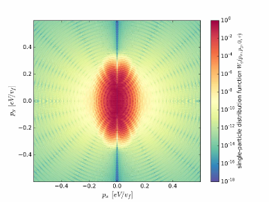
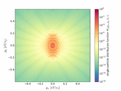
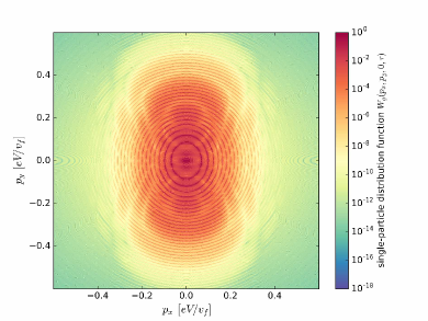
Figure 1: Logarithmic plot of the single-particle distribution functions $W_{\mathpzc{g}}(\boldsymbol{p},\tau)$. The result shown in the upper panel corresponds to a model involving massless charge carriers. Conversely, the middle and lower panels display outcomes obtained by considering massive Dirac quasiparticles. The distributions in the upper and middle panels follow from the strong field only, i.e. $E_{w}=0$, while the lower one takes into account that both the strong and the fast-oscillating waves are present. The following benchmark parameters have been used $\Delta\varepsilon=0.26\;\rm eV$, $E_{s}=4.9\times 10^{4}\ \rm V/cm$, $E_{w}=0.6\times 10^{4}\ \rm V/cm$, $N_{\mathrm{plateau}}=26$ cycles ($\tau\approx 4.2\ \rm ps$), $\Omega=0.026\ \rm eV$ and $\omega=0.206\ \rm eV$.

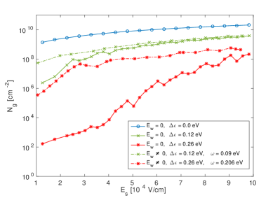
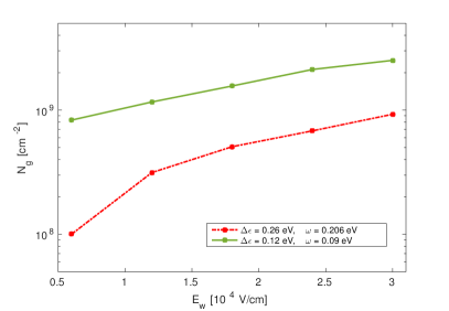
Figure 2: Density of produced electron-hole pairs as a function of $E_{s}$[left panel] and $E_{w}$[right panel]. The blue curve in the left panel reveals the trend obtained for the massless model when the weak field is off. For the same field setting, the lower curves in green and red – both with more pronounced slopes as compared with the remaining curves – result from considering massive Dirac quasiparticles with bandgaps $\Delta\varepsilon=0.12\ \rm eV$ and $\Delta\varepsilon=0.26\ \rm eV$, respectively. The corresponding outcomes resulting from the configuration assisted by the perturbative fast-oscillating wave share the previous color scheme but the curves are those containing asterisks. Both assisted curves have been obtained by setting $E_{w}=0.6\times 10^{4}\;\rm V/cm$. The results exhibited in both panels were obtained by setting the pulse length $N_{\mathrm{plateau}}=26\;\rm cycles$ ($\tau\approx 4.2\;\rm ps$) and the strong field frequency $\Omega=0.026\ \rm eV$. Besides, for $\Delta\varepsilon=0.26\ \rm eV$ the frequency of the perturbative field was chosen $\omega=0.206\ \rm eV$, whereas for $\Delta\varepsilon=0.12\ \rm eV$ we have utilized $\omega=0.09\ \rm eV$. The curves in the right panel have been obtained by considering the two previous gaps: green for $\Delta\varepsilon=0.12\;\rm eV$ and red for $\Delta\varepsilon=0.26\;\rm eV$. There the strong field was taken as $E_{s}=4.9\times 10^{4}\ \rm V/cm$ with $\Omega=0.026\ \rm eV$.

Now, we solve the system of differential equations (5) by varying the momentum components within the interval $-0.5\ \mathrm{eV}\leqslant p_{x,y}\mathpzc{v}_{f}\leqslant 0.5\ \mathrm{eV}$. The results of this analysis are displayed in Fig. 1 in a density color scheme which corresponds to $\log_{10}[W{g}(\boldsymbol{p},\tau)]$. While the upper panel shows the outcomes associated with the massless model, the consequences associated with the mass $\mathpzc{m}=11.7\ \mathrm{keV}/c^{2}$ can be evaluated by comparing with the middle panel. It is worth remarking that both pictures were generated by considering the effects due to the strong field only. Their main features – including the occurrence of a narrow vertical blue sector in the massless case – have been studied previously. For details, we refer the reader to Ref. Akal:2016stu . We note that these panels have been added here to facilitate – via comparisons – the understanding of the main outcome resulting from a scenario in which massive Dirac quasiparticles are produced by the combined effect of both the strong and the perturbative fast-oscillating wave [lower panel]. Observe that the three spectral densities are sharply anisotropic with respect to the momentum components, and manifest gradual decrements as both $p_{x}$ and $p_{y}$ increase. The stretching along $p_{y}$ is understood as a result of the minimal coupling between the external field and the quasiparticle via the kinetic momentum $p_{y}-e\mathpzc{A}(t)/c$, which enters into the quasienergy [see below Eq. (10)]. Hence, the creation of quasiparticle-hole pairs with rather large longitudinal momentum is more likely to take place.

All panels in Fig. 1 are characterized by ringlike structures which differ between each other. Each ring is understood as an isocontour of fixed quasienergy $\bar{\varepsilon}_{\boldsymbol{p}}$ satisfying the resonance condition in Eq. (10). The regions encompassed between two neighboring rings are characterized by less intense colors, this way indicating the formation of intermediate valleys. Observe that the outcome shown in the middle panel, i.e. for massive carriers with the fast-oscillating field turned off, looks rather different as compared with the model of massless Dirac quasiparticles [upper]. Clearly the number of resonances in the former is considerably smaller than in the latter case where the red-colored area is much more pronounced and compact. In view of this behavior, we can infer that the volume below the surface $W_{\mathpzc{g}}(p_{x},p_{y})$ will be substantially larger in the massless model [upper panel] than in the case where the Dirac quasiparticles are massive and only the strong field is on [middle panel]. As these volumes result from the integration over the momentum components, actually they will determine the number of yielded pairs per unit of area

$$\begin{split}\mathpzc{N}_{\;\mathpzc{g}}=&\lim_{t\to\infty}g_{s}g_{v}\int\frac{d^{2}p}{(2\pi)^{2}}\,W_{\mathpzc{g}}(\boldsymbol{p},t).\end{split}$$ (12)

We remark that the factor $g_{s}=2$ ($g_{v}=2$) accounts for the spin (valley) degeneracy. Formally, the integration has to be performed over all the Fourier space. However, the outcomes given in Fig. 1 provide evidences that the contribution of $W_{\;\mathpzc{g}}(\boldsymbol{p},\tau)$ is almost insignificant as long as $p_{x},\;p_{y}>10\;\mathrm{eV}/\mathpzc{v}_{f}$. This fact is consistent with the limitation indicated above Eq. (II). Hence, to compute Eq. (12) numerically we will restrict the integration domain to an area $A$ embedded within a circle with radius $|\boldsymbol{p}|\ll 10\ \mathrm{eV}/\mathpzc{v}_{f}$.

The situation changes when massive Dirac quasiparticles experience both the strong and the perturbative fast-oscillating wave simultaneously [lower panel]. Owing to the latter, the number of resonances increases and the red area enlarges considerably as compared with the panel in the middle. This fact makes clear that the corresponding volume below the surface $W_{\;\mathpzc{g}}(p_{x},p_{y})$, i.e. the density of produced electron-hole pairs, increases in comparison to the situation where $\mathpzc{m}=11.7\ \mathrm{keV}/c^{2}$ with the perturbative wave being switched off. Certainly, the red area in the lower panel turns out to be less intense than in the upper one [$\mathpzc{m}=0$]. However, in the former case, the red portion covers regions in the $(p_{x},p_{y})$-plane that the upper panel does not. Consequently, the volume enclosed by $W_{\;\mathpzc{g}}(p_{x},p_{y})$ in the assisted setting could reach values comparable to the one associated with the scenario involving massless carriers and, so for the density of created pairs [see Eq. (12)].

In order to verify this enhancement, we compute numerically the dependence of $\mathpzc{N}_{\;\mathpzc{g}}$ [see Eq. (12)] with respect to the strong electric field strength $E_{s}$. The results of this assessment are summarized in the left panel of Fig. 2. The outcome linked to the massless model is shown in blue, whereas those resulting from scenarios driven by massive Dirac quasiparticles characterized by a bandgap $\Delta\varepsilon=0.26\ \rm eV$ are depicted in red. For comparison, the results linked to a reduced gap $\Delta\varepsilon=0.12\ \rm eV$ have been included [green curves with an adjusted fast-oscillating frequency $\omega=0.09\;\rm eV$]. We note that the latter corresponds to a mass $\mathpzc{m}=5.4\;\mathrm{keV}/c^{2}$ and a critical field strength $E_{\mathpzc{g}}\approx 5.5\times 10^{4}\ \rm V/cm$ which is an order of magnitude smaller than the one associated with the energy gap $\Delta\varepsilon=0.26\ \rm eV$, i.e. $E{g}\approx 2.6\times 10^{5}\ \rm V/cm$. The right panel in Fig. 2 shows the dependence of $\mathpzc{N}_{\;\mathpzc{g}}$ on the weak field strength $E_{w}$. Each curve corresponds to one of the nontrivial bandgaps: green for $\Delta\varepsilon=0.12\;\rm eV$ and red for $\Delta\varepsilon=0.26\;\rm eV$. Both have been obtained by setting the strong field to $E_{s}=4.9\times 10^{4}\ \rm V/cm$. As the previous strength is comparable to the critical field linked to the gap $\Delta\varepsilon=0.12\;\rm eV$, the corresponding results have to be considered as estimates. Referring to the red curve, we see that the density of pairs grows from left to right by a factor of $\approx 20$ when the amplitude of the weak field is increased by a factor of 8, implying an average growth which is faster than linear. For comparison we note that, for PP by a bichromatic electric field in a pure QED context Akal:2014eua , a linear dependence on $E_{w}$ (respectively $\xi_{w}$) has been obtained to a good approximation. This simple scaling behavior may be attributed to the range of field parameters considered there.

Now, throughout the whole range of $E_{s}$ [left panel] the number of pairs yielded from the assisted scenario – green and red curves marked with asterisks – is substantially larger than those arising when the perturbative fast-oscillating field is off, i.e. green and red curves marked with crosses. We note that, in a scenario with an energy gap $\Delta\varepsilon=0.26\ \rm eV$ and $E_{s}\approx 2.7\times 10^{4}\;\rm V/cm$, the result of the assisted setup exceeds the outcome driven by a pure strong field setup by four orders of magnitude. For comparison we note that the presence of the assisting field [$E_{w}=0.6\times 10^{4}\;\rm V/cm$, $\omega=0.206\;\rm eV$] enhances the pair yield in the massless model by only a factor $2$, approximately. As – in average – the slopes of those curves linked to a pure strong field scenario [$\mathpzc{m}\neq 0$] are larger than the corresponding one in the assisted setting, the enhancement effect due to the weak field diminishes as $E_{s}$ grows [see also Refs. dgs2008 ; DiPiazza:2009py ; Jansen2013 ; Augustin2014 ]. This behavior can be expected because – in an assisted scenario – there are two paths for increasing the number of produced pairs. Namely, either by growing the strong field strength or through the absorption of energetic quanta, this way promoting the emergence of new resonances. While the former becomes more relevant as $E_{s}$ grows, the latter dominates as the opposite situation takes place.

Noteworthy, those curves linked to scenarios in which the production of massive electron-hole pairs is driven by the strong field only, manifest pronounced steep fallings which are caused by the so-called channel-closing effect [see, e.g., HReiss ; Kohlfurst:2013ura ; Akal:2014eua ; Akal:2016stu ]. Also the results associated with the assisted setups reveal these drop-offs, although much less noticeable due to the large scale covered by the vertical axis. We recall that the channel-closing phenomenon can be attributed to the extinction of a resonance at those field strengths for which $W_{\;\mathpzc{g}}(\boldsymbol{p},\tau)$ is locally minimized. Indeed, in the absence of a perturbative fast-oscillating wave, the number of produced pairs can increase through the growing of the strong field strength $E_{s}$. When this happens, the quasienergies that characterize the resonances [see below Eq. (10)] change too. Most of theses resonances – featured by a specific $n_{s}$ – survive during the electric field change because – when integrating over $\boldsymbol{p}$ – a readjustment in the corresponding momentum occurs in such a way that the relations $2\varepsilon_{\boldsymbol{p}}=n_{s}\Omega$ still hold. However, throughout the change, the minimal energy to be absorbed from the field – $\varepsilon_{\boldsymbol{p}=0}$ – might die out, this way compensating the enhancement induced by the strong field increment. If this occurs, the volume below the surface $W_{\;\mathpzc{g}}(p_{x},p_{y})$ diminishes and a drop-off emerges in the plane $(\mathpzc{N}_{\;\mathpzc{g}},E_{s})$. That this behavior does not manifest in the assisted curves may be then understood as a direct consequence of the additional production channel that the assisted scenario provides. Within the context of the resonant condition [see Eq. (10)], this manifests via the term which contains the number of quanta $n_{w}$ absorbed from the weak field.

Let us finally estimate the number of electron-hole pairs produced by a single shot in a sheet of graphene with a characteristic length $\ell\sim 10\;\mu\rm m$. Consider first the nonassisted scenario with $E_{s}\approx 5.6\times 10^{4}\;\rm V/cm$ and $\mathpzc{m}=11.7\;\mathrm{keV}/c^{2}$, for which $\mathpzc{N}_{\;\mathpzc{g}}\sim 10^{6}\;\rm cm^{-2}$. Under such circumstances the number of pairs created from the vacuum in a single shot is $\mathpzc{N}_{\;\mathpzc{g}}\ell^{2}\sim 1$ approximately. However, if the previous setup is assisted by a perturbative fast-oscillating wave with $\omega=0.206\ \rm eV$ and $E_{w}\approx 3\times 10^{4}\ \rm V/cm$, the density of pairs reaches values of the order of $\mathpzc{N}_{\;\mathpzc{g}}\sim 10^{8}\;\rm cm^{-2}$. As a consequence the number of electron-hole pairs produced by a single shot would be of the order of $N_{\mathrm{pairs}}\approx\mathpzc{N}_{\;\mathpzc{g}}\ell^{2}\sim 10^{2}$, i.e. two orders of magnitude larger than in the nonassisted configuration. The layer could accumulate a much larger number of electron-hole pairs by taking advantage of the laser repetition rate. For instance, values of the order of $N_{\mathrm{pairs}}\sim 10^{6}$ could be reached after $n_{\mathrm{shots}}\sim 10^{4}$ laser shots. For a repetition rate of $\nu\sim\mathcal{O}(10-100)\;\rm Hz$, this would require to irradiate the sample during $\mathcal{O}(2-17)\;\rm min$, approximately. After this period the density of produced electron-hole pairs reaches values of the order of $\mathpzc{N}_{\;f}=n_{\mathrm{shots}}\mathpzc{N}_{\;\mathpzc{g}}\sim 10^{12}\;\rm cm^{-2}$ which exceeds by $2$ orders of magnitude the density obtained from a single shot in a model with no gap [see blue curve, left panel in Fig. 2].

We note that for a final density $\mathpzc{N}_{\;f}\sim 10^{12}\;\rm cm^{-2}$ the electrostatic interactions becomes relevant Lewkovicz ; Ahiezer . This way facilitating the attraction between carriers with different charges and, thus, the formation of excitons i.e. the analog of the positronium in a pure QED context. As in the latter scenario, the formed excitons are expected to be unstable bound states which decay into photons. In first instance, the detection of these photons would constitute a direct signature of a prior realization of the assisted pair creation process. A study of the annihilation channels is beyond the scope of the present investigation, but they will be analyzed in a forthcoming publication.

IV Conclusion

Matter-antimatter pair creation via the Schwinger mechanism is one of the most striking nonperturbative phenomena in quantum field theory. Since it has eluded any experimental verification, so far, catalyzing mechanisms in nonstatic macroscopic gauge fields prove very promising in order to circumvent the dramatic suppression of the creation rate. Alternatively, one may also look for analog realizations in appropriate low energy condensed matter systems like graphene. In contrast to earlier studies, we have focused on scenarios where a tiny bandgap is present in the vicinity of its Dirac points, giving rise to the characteristic tunneling exponential in the Schwinger pair creation rate. This feature has allowed us to verify theoretically that such semiconducting graphene varieties are rather suitable not only to probe the Schwinger effect but also the proposed mechanism of dynamical assistance.

Employing a quantum kinetic approach with reduced effective dimensionality, we first have computed the corresponding single-particle distribution function for experimentally motivated field parameters. In doing so, we have verified that the presence of an assisting weak field can yield a notably enhancement, approaching values obtained for ordinary massless graphene via the standard PP mechanism. For all configurations a characteristic resonant behavior, reflected in form of isocontours of fixed quasienergy, has been identified in the momentum plane. Based on the obtained distribution functions, we then have computed the total number of created quasiparticle-hole pairs. We have shown that the latter enabled via the assisted mechanism turned out to be several orders of magnitude larger than in the nonassisted process. We have argued that, with a suitable laser repetition rate, the density of produced electron-hole pairs increases by several orders of magnitude, allowing to reach the level from which the emission of photons – as a result of the recombination process – becomes a clear signature of the assisted Schwinger mechanisms.

References

- (1)
- (2) F. Sauter, Über das Verhalten eines Elektrons im homogenen elektrischen Feld nach der relativistischen Theorie Diracs, Z. Phys. 69, 742 (1931).
- (3) W. Heisenberg and H. Euler, Folgerungen aus der Diracschen Theorie des Positrons, Z. Phys. 98, 714 (1936).
- (4) J. S. Schwinger, On gauge invariance and vacuum polarization, Phys. Rev. 82, 664 (1951).
- (5) See: http://www.eli-laser.eu
- (6) See: http://www.xcels.iapras.ru/
- (7) F. Hebenstreit and F. Fillion-Gourdeau, Optimization of Schwinger pair production in colliding laser pulses, Phys. Lett. B 739, 189 (2014).
- (8) S. S. Bulanov, V. D. Mur, N. B. Narozhny, J. Nees, and V. S. Popov, Multiple colliding electromagnetic pulses: a way to lower the threshold of pair production from vacuum, Phys. Rev. Lett. 104, 220404 (2010).
- (9) R. Schützhold, H. Gies and G. Dunne, Dynamically assisted Schwinger mechanism, Phys. Rev. Lett 101, 130404 (2008).
- (10) G. Dunne, H. Gies and R. Schützhold, Catalysis of Schwinger vacuum pair production, Phys. Rev. D 80, 111301 (2009).
- (11) M. Orthaber, F. Hebenstreit, and R. Alkofer, Momentum spectra for dynamically assisted Schwinger pair production, Phys. Lett. B 698, 80 (2011).
- (12) M. Jiang, W. Su, Z. Q. Lv, X. Lu, Y. J. Li, R. Grobe, and Q. Su, Pair creation enhancement due to combined external fields, Phys. Rev. A 85, 033408 (2012).
- (13) I. Akal, S. Villalba-Chávez and C. Müller, Electron-positron pair production in a bifrequent oscillating electric field, Phys. Rev. D 90, 113004 (2014).
- (14) A. Otto, D. Seipt, D. Blaschke, B. Kämpfer, S. A. Smolyansky, Lifting shell structures in the dynamically assisted Schwinger effect in periodic fields, Phys. Lett. B 740, 335 (2014).
- (15) A. D. Panferov, S. A. Smolyansky, A. Otto, B. Kämpfer, D. B. Blaschke, and Ł. Juchnowski, Assisted dynamical Schwinger effect: pair production in a pulsed bifrequent field, Eur. Phys. J. D 70, 56 (2016).
- (16) M. F. Linder, C. Schneider, J. Sicking, N. Szpak, and R. Schützhold, Pulse shape dependence in the dynamically assisted Sauter-Schwinger effect, Phys. Rev. D 92, 085009 (2015).
- (17) G. Torgrimsson, J. Oertel, and R. Schützhold, Doubly assisted Sauter-Schwinger effect, Phys. Rev. D 94, 065035 (2016).
- (18) I. Akal, G. Moortgat-Pick, Euclidean mirrors: enhanced vacuum decay from reflected instantons, J. Phys. G 45, 055007 (2018).
- (19) A. Di Piazza, E. Lötstedt, A. I. Milstein and C. H. Keitel, Barrier control in tunneling - photoproduction, Phys. Rev. Lett. 103, 170403 (2009).
- (20) M. J. A. Jansen and C. Müller, Strongly enhanced pair production in combined high- and low-frequency laser fields, Phys. Rev. A 88, 052125 (2013).
- (21) S. Augustin and C. Müller, Nonperturbative Bethe-Heitler pair creation in combined high- and low-frequency laser fields, Phys. Lett. B 737, 114 (2014).
- (22) S. Y. Zhou et al., Substrate-induced bandgap opening in epitaxial graphene, Nature Materials 6, 770 (2007).
- (23) G. Giovannetti, P. A. Khomyakov, G. Brocks, P. J. Kelly, and J. van den Brink, Substrate-induced band gap in graphene on hexagonal boron nitride: Ab initio density functional calculations, Phys. Rev. B 76, 073103 (2007).
- (24) D. N. Basov, M. M. Fogler, A. Lanzara, F. Wang, and Y. Zhang, Colloquium: Graphene Spectroscopy, Rev. Mod. Phys. 86, 959 (2014).
- (25) A. Varykhalov, J. Sánchez-Barriga, A. M. Shikin, C. Biswas, E. Vescovo, A. Rybkin, D. Marchenko, and O. Rader, Electronic and Magnetic Properties of Quasifreestanding Graphene on Ni, Phys. Rev. Lett. 101, 157601 (2008).
- (26) I. V. Oladyshkin, S. B. Bodrov, Yu. A. Sergeev, A. I. Korytin, M. D. Tokman, and A. N. Stepanov, Optical emission of graphene and electron-hole pair production induced by a strong terahertz field, Phys. Rev. B. 96, 155401 (2017).
- (27) Ch. Lui, K. F. Mak, J. Shan, and T. F. Heinz, Ultrafast photoluminicence from graphene, Phys. Rev. Lett. 105, 127404 (2010).
- (28) S. Tani, F. Blanchard, and K. Tanaka, Ultrafast carrier Dynamics in graphene under a high electric field, Phys. Rev. Lett. 109, 166603 (2012).
- (29) P. R. Wallace, The band theory of graphite, Phys. Rev. 71, 622 (1947).
- (30) I. Akal, R. Egger, C. Müller, and S. Villalba-Chávez, Low-dimensional approach to pair production in an oscillating electric field: Application to bandgap graphene layers, Phys. Rev. D 93, 116006 (2016).
- (31) M. F. Linder, A. Lorke and R. Schützhold, Analog Sauter-Schwinger effect in semiconductors for spacetime-dependent fields, Phys. Rev. B 97, 035203 (2018).
- (32) D. Allor, T. D. Cohen and D. A. McGady, The Schwinger mechanism and graphene, Phys. Rev. D 78, 096009 (2008).
- (33) G. L. Klimchitskaya, and V. M. Mostepanenko, Creation of quasiparticles in graphene by a time-dependent electric field, Phys. Rev. D 78, 096009 (2008).
- (34) H. K. Avetissian, A. K. Avetissian, G. F. Mkrtchian and Kh. V. Sedrakian, Creation of particle-hole superposition states in graphene at multiphoton resonant excitation by laser radiation, Phys. Rev. B 85, 115443 (2012).
- (35) F. Fillion-Gourdeau and S. MacLean, Time-dependent pair creation and the Schwinger mechanism in graphene, Phys. Rev. B 92, 035401 (2015).
- (36) F. Fillion-Gourdeau, D. Gagnon, C. Lefebvre and S. MacLean, Time-domain quantum interference in graphene, Phys. Rev. B 94, 125423 (2016).
- (37) K. S. Novoselov, et al., Electric Field effect in atomically thin Carbon films, Science 306, 666 (2004).
- (38) K. S. Novoselov et al., Two-dimensional atomic crystals, Proc. Natl. Acad. Sci. 102, 10451 (2005).
- (39) K. S. Novoselov et al., Two-dimensional gas of massless Dirac fermions in graphene, Nature 438, 197 (2005).
- (40) D. M. Gitman Processes of arbitrary order in quantum electrodynamics with a pair-creating external field, J. Phys. A 10, 2007 (1977).
- (41) E. S. Fradkin, D. M. Gitman, and S. M. Shvartsman, Quantum Electrodynamics with Unstable Vacuum (Springer-Verlag, Berlin, 1991).
- (42) D. V. Vinnik, A. V. Prozorkevich, S. A. Smolyansky, V. D. Toneev, C. D. Roberts, and S. M. Schmidt, Plasma production and thermalization in a strong field, Eur. Phys. J. C 22, 341 (2001).
- (43) J. C. R. Bloch, V. A. Mizerny, A. V. Prozorkevich, C. D. Roberts, S. M. Schmidt, S. A. Smolyansky, D. V. Vinnik, Pair creation: Back reactions and damping, Phys. Rev. D 60, 116011 (1999).
- (44) N. Tanji, Dynamical view of pair creation in uniform electric and magnetic fields, Annals Phys. 324, 1691 (2009).
- (45) F. Hebenstreit, R. Alkofer and H. Gies, Schwinger pair production in space- and time-dependent electric fields: Relating the Wigner formalism to quantum kinetic theory, Phys. Rev. D 82, 105026 (2010).
- (46) G. R. Mocken, M. Ruf, C. Müller and C. H. Keitel, Nonperturbative multiphoton electron-positron-pair creation in laser fields, Phys. Rev. A 81, 022122 (2010).
- (47) D. J. Cook and R. M. Hochstrasser, Intense terahertz pulses by four-wave rectification in air, Opt. Lett. 25, 1210 (2000).
- (48) T. Bartel, P. Gaal, K. Reimann, M. Woerner, and T. Elsaesser, Generation of single-cycle THz transients with high electric-field amplitudes, Opt. Lett. 30, 2805 (2005).
- (49) H. R. Reiss, Special analytical properties of ultrastrong coherent fields, Eur. Phys. J. D 55, 365-374 (2009).
- (50) C. Kohlfürst, H. Gies, and R. Alkofer, Effective mass signatures in multiphoton pair production, Phys. Rev. Lett. 112, 050402 (2014).
- (51) A. I. Ahiezer, and V. B. Beresteckiy, Quantum electrodynamics, Nakua, Moscow (1981).
- (52) M. Lewkovicz, H. C. Kao, and B. Rosentein, Signature of the Schwinger pair creation rate via radiation generated in graphene by strong electric current, Phys. Rev. B. 84, 035414 (2011).