The hadronic vacuum polarization contribution to $(g-2)_{\mu}$ from 2 + 1 flavours of O($a$) improved Wilson quarks

Abstract:

We report on our ongoing project to determine the leading-order hadronic vacuum polarisation contribution to the muon $g-2$, using ensembles with $N_{\rm f}=2+1$ flavours of O($a$) improved Wilson quarks generated by the CLS effort, with pion masses down to the physical value. We employ O($a$) improved versions of the local and conserved vector currents to compute the contributions of the light, strange and charm quarks to $(g-2)_{\mu}$, using the time-momentum representation. We perform a detailed investigation of the systematic effects arising from constraining the long-distance regime of the vector correlator. To this end we make use of auxiliary calculations in the iso-vector channel using distillation and the Lüscher formalism. Our results are corrected for finite-volume effects by computing the timelike pion form factor in finite and infinite volume. For certain parameter choices, the corrections computed in this way can also be confronted with results determined on different volumes. Currently, the overall precision of our results is limited by the uncertainties in the lattice scale.

1 Introduction

The persistent discrepancy of $\approx 3.5$ standard deviations between the direct measurement of the muon’s anomalous magnetic moment $a_{\mu}=\frac{1}{2}(g-2)_{\mu}$ and the value predicted by theory [1] is one of the most promising hints for physics beyond the Standard Model. In view of the fact that the experimental precision is set to increase by a factor four, owing to the efforts by the Fermilab E989 and J-PARC E34 experiments, it is of paramount importance to reduce the error of the theoretical prediction. Lattice QCD calculations have emerged as a promising method to obtain estimates for both the hadronic vacuum polarisation and light-by-light scattering contributions, $a_{\mu}^{\rm hvp}$ and $a_{\mu}^{\rm hlbl}$, with controlled uncertainties (see the recent review in [2]). In Ref. [3] we published a result for $a_{\mu}^{\rm hvp}$ in two-flavour QCD, i.e.

$$a_{\mu}^{\rm hvp}=(654\pm 32\,{{}^{+21}_{-23}})\cdot 10^{-10},$$ (1)

where the first error is statistical and the second represents a combination of various systematic errors. Clearly, the total precision of $\approx 6$ % is insufficient to have an impact on resolving the $g-2$ puzzle. Here we report on our ongoing effort to determine $a_{\mu}^{\rm hvp}$ in lattice QCD with $N_{\rm f}=2+1$ flavours of O($a$) improved Wilson fermions. Previous accounts have been given in [4] and [2].

2 Features of our calculation

Our evaluation of $a_{\mu}^{\rm hvp}$ is based on the time-momentum representation (TMR) [5], i.e.

$$a_{\mu}^{\rm hvp}=\left(\frac{\alpha}{\pi}\right)^{2}\int_{0}^{\infty}dx_{0}\,\tilde{K}(x_{0})G(x_{0}),$$ (2)

where $\tilde{K}(x_{0})$ is a known kernel function depending on the Euclidean time $x_{0}$ [5, 3], and $G(x_{0})$ is the spatially summed correlator of two electromagnetic currents

$$G(x_{0})=-a^{3}\sum_{\vec{x}}\,\left\langle J_{k}(x)J_{k}(0)\right\rangle,\quad J_{\mu}(x)={\textstyle\frac{2}{3}}\bar{u}\gamma_{\mu}u-{\textstyle\frac{1}{3}}\bar{d}\gamma_{\mu}d-{\textstyle\frac{1}{3}}\bar{s}\gamma_{\mu}s+\ldots.\vspace{-0.2cm}$$ (3)

Previous calculations suggest that the tail of the integrand $\tilde{K}(x_{0})G(x_{0})$, i.e. the region $x_{0}\gtrsim 3$ fm makes a sizeable contribution of about 3% to $a_{\mu}^{\rm hvp}$. Hence, in order to determine $a_{\mu}^{\rm hvp}$ with sufficient precision, it is important to accurately constrain the long-distance regime of the correlator $G(x_{0})$, which is dominated by the two-pion contribution to the iso-vector component.

Below we sketch the main features of our calculation. We employ the gauge ensembles generated as part of the CLS effort, using $N_{\rm f}=2+1$ flavours of O($a$) improved Wilson quarks [6]. In order to combat the problem of topology freezing, a large fraction of the ensembles have open boundary conditions in the time direction [7, 8]. The hopping parameters of the dynamical light and strange quarks were chosen such that the physical point is reached along a trajectory where ${\rm Tr}\,M=\rm const$. Further details of the 17 ensembles used in this study are listed in Table 1: we have computed $a_{\mu}^{\rm hvp}$ for four different lattice spacings, covering a range of pion masses from around 400 MeV down to the physical one. While all ensembles satisfy $m_{\pi}L\geq 4$, we can also study finite-volume effects by comparing results at different volumes for fixed $m_{\pi}$. The lattice scale is set via the gradient flow time, which has been determined in [9] as $\sqrt{8t_{0}}=0.415(4)(2)$ fm. The current uncertainty of the scale determination of about 1% limits the overall precision of our calculation of $a_{\mu}^{\rm hvp}$ (see the discussion on the scale setting error in [3, 4]).

In order to constrain the long-distance regime of the vector correlator, we have performed a dedicated calculation of the light-quark iso-vector correlator, employing correlator matrices and the distillation technique [10, 11], which allows not only for the determination of the $I=1$ scattering phase shift but also of the timelike pion form factor [12]. For the evaluation of quark-disconnected diagrams we have resorted to using hierarchical probing [13], as well as a new covariant coordinate space technique [14].

ensemble	BCs	$\beta$	$a$ [fm]	$L/a$	$T/a$	$L$ [fm]	$m_{\pi}$ [MeV]	$m_{\pi}L$
H101	obc	3.40	0.0865	32	96	2.77	420	5.9
H102	obc			32	96	2.77	350	4.9
H105	obc			32	96	2.77	280	3.9
N101	obc			48	128	4.15	280	5.9
C101	obc			48	96	4.15	220	4.6
B450	pbc	3.46	0.0765	32	64	2.45	415	5.2
S400	obc			32	128	2.45	350	4.3
N401	obc			48	128	3.67	280	5.2
H200	obc	3.55	0.0644	32	96	2.06	420	4.4
N202	obc			48	128	3.09	420	6.6
N203	obc			48	128	3.09	340	5.3
N200	obc			48	128	3.09	280	4.4
D200	obc			64	128	4.12	200	4.2
E250	pbc			96	192	6.18	135	4.2
N300	obc	3.70	0.0499	48	128	2.40	420	5.1
N302	obc			48	128	2.40	340	4.1
J303	obc			64	192	3.19	260	4.2

Table 1: Simulation parameters and pion masses of the ensembles used in this study. The labels “obc” and “pbc” indicate the use of open or periodic boundary conditions, respectively.

In our calculations we employ the O($a$) improved versions of the local (loc) and conserved (con) vector currents. For the local current, $V_{\mu}^{\rm loc}(x)=(\bar{\psi}\gamma_{\mu}\psi)(x)$, the expression is

$$(V_{\mu}^{\rm loc}(x))^{I}=V_{\mu}^{\rm loc}(x)+ac_{\rm V}^{\rm loc}\,\tilde{\nabla}_{\nu}T_{\mu\nu}(x),\vspace{-0.1cm}$$ (4)

where $T_{\mu\nu}=-\frac{1}{2}\bar{\psi}[\gamma_{\mu},\gamma_{\nu}]\psi$ is the tensor current, $\tilde{\nabla}_{0}$ denotes the symmetrised lattice derivative, and $c_{\rm V}^{\rm loc}$ is an improvement coefficient that can be evaluated non-perturbatively by imposing chiral Ward identities [15, 16]. There is an analogous expression for the improved conserved current, with coefficient $c_{\rm V}^{\rm con}$. The local vector current must be renormalised, and in this contribution we employ the non-perturbative determination of the renormalisation factor $Z_{\rm V}$ from ratios of three- and two-point correlation functions, similarly to our two-flavour calculation [3]. The expression of the (mixed) correlator involving the conserved and local currents for quark flavour $f$ reads

$$G^{lc}_{f}(x_{0})=-\frac{a^{3}}{3}\sum_{k=1}^{3}\sum_{\vec{x}}{q}_{f}^{2}\,Z_{\rm V}\left\langle V_{k,f}^{\rm con}(x_{0},\vec{x})V_{k,f}^{\rm loc}(0)\right\rangle,\qquad f=ud,s,c,\vspace{-0.2cm}$$ (5)

where $V_{k,f}$ denotes the spatial component of the vector current of flavour $f$, and ${q}_{f}$ is the corresponding electric charge. Note that only quark-connected contributions are included in Eq. (5). We also consider the correlator $G^{ll}_{f}(x_{0})$ of two local currents, which contains a factor of $Z_{\rm V}^{2}$.

A recent analysis of the renormalisation pattern of the improved local vector current has shown that SU(3) flavour breaking induces a mixing between the local vector currents of different quark flavours at O($a$) [16]. Hence, in order to be consistent with improvement, the contributions of individual quark flavours to $a_{\mu}^{\rm hvp}$ must be derived from linear combinations of correlators of appropriately renormalised quark currents. The findings of Ref. [16] were not available at the time of the conference, and we leave the full analysis to a later publication.

3 Preliminary results

In the left panel of Fig. 2 we show the integrand $\tilde{K}(x_{0})G^{ll}_{ud}(x_{0})$ on ensemble D200, at a pion mass of about 200 MeV. The data, denoted by black points, are compared to the results of our auxiliary calculation of the iso-vector correlator $G^{\rho\rho}(x_{0},L)$, whose long-distance behaviour is

$$G^{\rho\rho}(x_{0},L)\stackrel{{\scriptstyle x_{0}\gg 0}}{{\sim}}\sum_{n}\,|A_{n}|^{2}\,{\rm e}^{-\omega_{n}x_{0}},\qquad\omega_{n}=2\sqrt{m_{\pi}^{2}+k^{2}},$$ (6)

where $k$ is the scattering momentum. The energy levels $\omega_{n}$ were determined for the four lowest-lying states by computing correlator matrices using $\rho$ and $\pi\pi$ interpolating operators and stochastic distillation [11] and solving the associated generalised eigenvalue problem. In a second step, the amplitude $A_{n}\equiv\langle 0|V_{k,ud}^{\rm con}(0)|n\rangle$ was determined as the matrix element of the local current and the approximate interpolator onto the $n^{\rm{th}}$ energy eigenstate $|n\rangle$. From the figure it is clear that the accumulated contributions from the four lowest-lying states saturate the iso-vector correlator for $x_{0}\gtrsim 1$ fm. Furthermore, the long-distance behaviour of the integrand $\tilde{K}(x_{0})G^{ll}_{ud}(x_{0})$ is well described by the iso-vector contribution which is also statistically more accurate. Finally, one concludes that the two-pion contribution, denoted by the red filled circles, dominates the vector correlator for $x_{0}\gtrsim 3$ fm.

The long-distance behaviour of the vector correlator is closely related to the important issue of finite-volume effects. In [17, 3] it was shown how finite-volume corrections can be computed by inserting the difference of the isovector correlator in finite and infinite volume into the integral representation Eq. (2). For the latter, the expression is

$$G^{\rho\rho}(x_{0},\infty)=\int_{0}^{\infty}d\omega\,\omega^{2}\,\rho(\omega^{2})\,{\rm e}^{-\omega|x_{0}|},\quad\rho(\omega^{2})=\frac{1}{48\pi^{2}}\left(1-\frac{4m_{\pi}^{2}}{\omega^{2}}\right)^{3/2}\left|F_{\pi}(\omega)\right|^{2},$$ (7)

where $\rho(\omega^{2})$ denotes the spectral function, which is related to the timelike pion form factor $F_{\pi}(\omega)$. In the absence of any direct lattice calculation of $F_{\pi}(\omega)$ one may resort to the Gounaris-Sakurai (GS) parameterisation [18]. Obviously, it is important to verify the predictions of the GS model by confronting them with lattice data obtained on different volumes. In the right panel of Fig. 2 we compare the TMR integrand computed on ensembles H105 and N101, which realise the same pion mass ($m_{\pi}=280$ MeV) on two different volumes, corresponding to ${m_{\pi}}L=3.9$ and 5.9, respectively. One then finds that the finite-volume correction determined by the GS model is tiny for the larger volume (N101). Second, one finds that the FV-corrected data on the smaller volume (H105) agree with those on N101 within errors. We conclude that finite-size effects are well described by the GS parameterisation of $F_{\pi}(\omega)$. At the physical pion mass and for $m_{\pi}L=4$, which corresponds to our ensemble E250, we estimate a finite-volume correction to $a_{\mu}^{\rm hvp}$ of $(20\pm 4)\cdot 10^{-10}$ using the GS model. It is interesting to note that this correction is reduced by a factor 10 for $m_{\pi}L=6$. A calculation of the timelike pion form factor has been performed for a subset of our previously studied two-flavour ensembles [19]. The implications for $a_{\mu}^{\rm hvp}$ will be discussed in a forthcoming publication [20].

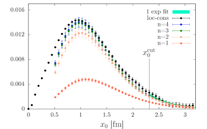
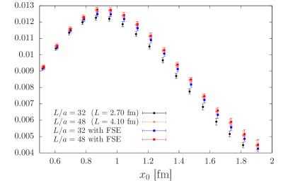
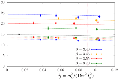
Figure 1: Left: The integrand $\tilde{K}(x_{0})G^{ll}_{ud}(x_{0})$ on ensemble D200 in units of $m_{\mu}$, compared to the iso-vector contribution $\tilde{K}(x_{0})G^{\rho\rho}(x_{0},L)$. Right: the integrand $\tilde{K}(x_{0})G^{lc}_{ud}(x_{0})$ computed on ensembles H105 and N101, before and after applying the finite-volume correction computed using the Gounaris-Sakurai parameterisation of $F_{\pi}(\omega)$.

Figure 2: Chiral and continuum extrapolations of the contributions of the charm (left) and light quarks (right) to $a_{\mu}^{\rm hvp}$, in units of $10^{-10}$. Data points are plotted versus the variable $\tilde{y}=m_{\pi}^{2}/(16\pi^{2}f_{\pi}^{2})$. Solid and dotted lines describe the pion mass dependence of the results determined from the local-local and local-conserved correlators, respectively. Estimates at the physical point are represented by black circles.

In Fig. 2 we show examples of our combined chiral and continuum extrapolations for the charm and light quark contributions. We perform a simultaneous extrapolation of the results obtained from the local-conserved and local-local correlator to a common value at the physical point, based on the fit function $f(m_{\pi},\beta)=\alpha_{1}+\alpha_{2}m_{\pi}^{2}+\alpha_{3}m_{\pi}^{2}\ln m_{\pi}^{2}+\alpha_{4}a^{2}$. One finds that the availability of two different discretisations of the correlator leads to a much more reliable extrapolation, in particular in the case of the charm quark contribution for which discretisation effects are quite large. Owing to the fact that the hopping parameter corresponding to the bare charm quark mass has not been determined yet on ensemble E250, there is currently no direct result at the physical pion mass. Restricting the analysis to the connected contribution only, we obtain the following estimates for the light, strange and charm quark contributions at the physical point:

$$(a_{\mu}^{\rm hvp})^{ud}=643(21)\cdot 10^{-10},\quad(a_{\mu}^{\rm hvp})^{s}=52.6(2.5)\cdot 10^{-10},\quad(a_{\mu}^{\rm hvp})^{c}=14.95(47)\cdot 10^{-10}.$$ (8)

The quoted statistical errors are dominated by the uncertainty in the lattice scale.

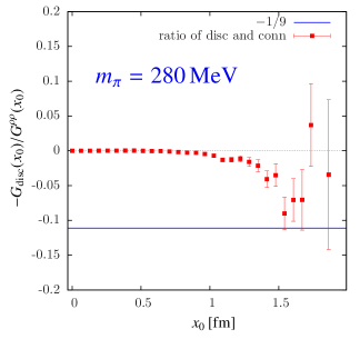
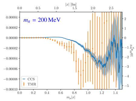
Figure 3: Left: The ratio of the disconnected over the connected light quark contribution (red circles) compared to the asymptotic value of $-1/9$ (blue horizontal line) for ensemble N200. Right: Comparison of the accumulated disconnected contribution determined using the TMR (orange circles) and the CCS method (blue band) for ensemble D200.

We have also computed the contributions from quark-disconnected diagrams, employing the technique of hierarchical probing with Hadamard vectors [13]. As in our previous calculation we took advantage of the cancellation of stochastic noise between light and strange quark loops [21]. In the left panel of Fig. 3 we plot the ratio $-G_{\rm{disc}}(x_{0})/G^{\rho\rho}(x_{0})$ of the disconnected and the light quark connected isovector contribution. As shown in [3], this ratio approaches the value $-1/9$ as $x_{0}\to\infty$, and indeed we see the onset of the expected asymptotic behaviour in the data. In the right panel we display a comparison of the accumulated disconnected contribution to $a_{\mu}^{\rm hvp}$ computed using our standard method to the results obtained using the covariant coordinate space (CCS) method of Ref. [14], which was also applied in a calculation of the hadronic corrections to the weak mixing angle [22]. While both techniques give consistent results, the CCS method is statistically more accurate.

4 Conclusions

Adding the contributions from light, strange and charm quarks in Eq. (8) we obtain our preliminary result of $a_{\mu}^{\rm hvp}=711\cdot 10^{-10}$, with an error of about 3% which is dominated by scale setting. Our calculation will be improved further by increasing statistics, the inclusion of the contribution from quark-disconnected diagrams and the effects from strong and electromagnetic isospin breaking. Details of our calculational framework can be found in Refs. [23, 24].

Acknowledgments: Our calculations were performed on the HPC Clusters Wilson, Clover and MOGON-II at the University of Mainz, on the JUQUEEN computer at NIC, Jülich (Project HMZ21) and on Hazel Hen at HLRS, Stuttgart (Project GCS-HQCD, Acid 44131). We thank Marco Cè for providing the plot of the right-hand panel in Fig. 3. KO is supported by DFG grant HI 2014/1-1. We thank our colleagues within the CLS initiative for sharing ensembles.

References

- [1] Particle Data Group, M. Tanabashi et al., Phys. Rev. D98 (2018) 030001.
- [2] H. B. Meyer and H. Wittig, Prog. Part. Nucl. Phys. 104 (2019) 46 [1807.09370].
- [3] M. Della Morte, A. Francis, V. Gülpers, G. Herdoíza, G. von Hippel, H. Horch et al., JHEP 10 (2017) 020 [1705.01775].
- [4] M. Della Morte et al., EPJ Web Conf. 175 (2018) 06031 [1710.10072].
- [5] D. Bernecker and H. B. Meyer, Eur. Phys. J. A47 (2011) 148 [1107.4388].
- [6] M. Bruno et al., JHEP 02 (2015) 043 [1411.3982].
- [7] ALPHA collaboration, S. Schaefer, R. Sommer and F. Virotta, Nucl. Phys. B845 (2011) 93 [1009.5228].
- [8] M. Lüscher and S. Schaefer, JHEP 1107 (2011) 036 [1105.4749].
- [9] M. Bruno, T. Korzec and S. Schaefer, Phys. Rev. D95 (2017) 074504 [1608.08900].
- [10] Hadron Spectrum collaboration, M. Peardon, J. Bulava, J. Foley, C. Morningstar, J. Dudek, R. G. Edwards et al., Phys. Rev. D80 (2009) 054506 [0905.2160].
- [11] C. Morningstar, J. Bulava, J. Foley, K. J. Juge, D. Lenkner, M. Peardon et al., Phys. Rev. D83 (2011) 114505 [1104.3870].
- [12] H. B. Meyer, Phys. Rev. Lett. 107 (2011) 072002 [1105.1892].
- [13] A. Stathopoulos, J. Laeuchli and K. Orginos, 1302.4018.
- [14] H. B. Meyer, Eur. Phys. J. C77 (2017) 616 [1706.01139].
- [15] M. Guagnelli and R. Sommer, Nucl. Phys. Proc. Suppl. 63 (1998) 886 [hep-lat/9709088].
- [16] A. Gérardin, T. Harris and H. B. Meyer, 1811.08209.
- [17] A. Francis, B. Jäger, H. B. Meyer and H. Wittig, Phys. Rev. D88 (2013) 054502 [1306.2532].
- [18] G. J. Gounaris and J. J. Sakurai, Phys. Rev. Lett. 21 (1968) 244.
- [19] F. Erben, J. Green, D. Mohler and H. Wittig, EPJ Web Conf. 175 (2018) 05027 [1710.03529].
- [20] F. Erben, J. Green, D. Mohler and H. Wittig, in preparation, .
- [21] V. Gülpers, A. Francis, B. Jäger, H. Meyer, G. von Hippel and H. Wittig, PoS LATTICE2014 (2014) 128 [1411.7592].
- [22] M. Cè, A. Gérardin, K. Ottnad and H. B. Meyer, PoS LATTICE2018 (2018) 137 [1811.08669].
- [23] A. Risch and H. Wittig, EPJ Web Conf. 175 (2018) 14019 [1710.06801].
- [24] A. Risch and H. Wittig, PoS LATTICE2018 (2018) 059 [1811.00895].