Positive and Negative Photospheric Fields in Solar Cycles 21 - 24

1 Introduction

All variety of manifestations of the solar activity (SA) is related to magnetic fields of various strength and their localization on the surface of the Sun. The distribution of magnetic fields over the surface of the Sun and its change in the course of the solar cycle is one of the key points in creating of the solar dynamo models (see, for example, Charbonneau, 2010). Evolution of zonal distribution of the Sun’s magnetic field was considered by Hoeksema (1991) on the basis of magnetograms of the Wilcox Solar Observatory (WSO). It was shown that the magnetic flux is closely connected to the level of activity and is similar to the Maunder butterfly diagram which reflects the distribution of sunspots. Variations of magnetic fields in time and latitude are considered by Akhtemov et al. (2015) where the strong difference of variations of the magnetic flux at low and high latitudes is revealed.

In contrast to the 11-year solar cycle which shows itself in the increase and following decrease of the number and area of sunspots, the 22-year recurrence of the magnetic field is observed as changes in polarity of the solar magnetic fields: sign change of the leading and following sunspots in the solar cycle minimum (Hale’s law), sign change of the polar field near SA maximum. Thus, the polarity of magnetic fields of the Sun is important characteristic of many processes, which are connected with the recurrence of SA.

Field lines of the magnetic field are closed, therefore the magnetic fluxes of the Sun of the positive and negative polarity have to be equal. However by consideration of separate manifestations of SA the balance of polarity is often broken. For example, the imbalance of magnetic fields of the leading and following sunspots is a well-known fact. In Cycle 21 at the northern/southern active regions the positive/negative fields were on average stronger, than negative/positive (Petrie, 2012). During Cycle 22 the situation was opposite, and the picture returned again to initial when Cycle 23 began. These relations reflect widely known fact that magnetic fields of bipolar groups of sunspots display the asymmetry with the leading polarity being as a rule stronger.

The imbalance is observed also in the polar fields which are antisymmetric except for some abnormal periods. During the reversal of the polar field the two hemispheres develop rather independently, therefore polar fields do not complete the change of sign reversals synchronously (Svalgaard and Kamide, 2013). In some periods the global field of the Sun lost the dipole character and looked as a monopole (Wilcox, 1972; Kotov, 2009).

The dipole character of the global field is manifested in the defining role of the dipole moment among coefficients of the magnetic field multipole expansion according to the PFSS model (the potential-field source-surface model (Hoeksema and Scherrer, 1986)). The dominating terms of the expansion are the dipole, hexapole, and quadrupole, the main field components during minima of SA being the axial ones (Bravo and González-Esparza, 2000). While the dipole and hexapole have opposite polarities at the Sun’s poles, the quadrupole has the same sign at both poles. In each minimum of SA the polarity of the quadrupole is opposite to the dipole and the hexapole polarity in the north and coincides with the polarity of the dipole and the hexapole in the south. Because of this property the quadrupole moment increases the polar magnetic field of the southern hemisphere, at the same time weakening the polar field of the northern hemisphere which results in asymmetry of the magnetic field of the Sun. Weak magnetic fields occupy most of the solar surface. Ioshpa, Obridko, and Chertoprud (2009) showed that small-scale background magnetic fields form a population which has a tendency to specific cyclic variations.

Exploring the imbalance of the positive and negative magnetic fields we take into consideration only the sign of the field, irrespective of the field strength. Due to this approach the fields with the weak and average strength are observed more distinctly, because only the surface area occupied with fields of certain polarity was taken into account. The purpose of this research was studying of the distribution of the photospheric fields with opposite polarities over the solar surface and the change of this distribution during a 22-year magnetic cycle.

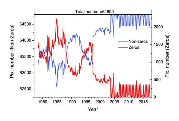
Figure 1.: The number of zero (red line) and non-zero (blue line) values of the magnetic field strength in synoptic maps (number of pixels). Each map consists of 64800 pixels. Data of KPVT: $1978-2003$; data of SOLIS: $2003-2016$. zeros

2 Data and method

We used as basic data synoptic maps of the photospheric magnetic field of National Solar Observatory Kitt Peak (NSO Kitt Peak). Combining the data obtained by two instruments of the Kitt Peak Observatory - KPVT (Kitt Peak Vacuum Telescope) for $1976-2003$ (ftp://nispdata.nso.edu/kpvt/synoptic/mag/) and SOLIS/VSM (Synoptic Optical Long-term Investigations of the Sun, Vector Solar Magnetometer) for $2003-2016$ (https://magmap.nso.edu/solis/archive.html) we studied the change of positive and negative magnetic fields during four solar cycles. Synoptic maps of the photospheric magnetic field are produced with the resolution of $1^{\circ}$ of the longitude (360 steps) and 180 equal steps in the sine of the latitude. Thus, each map contained 360x180 pixels of magnetic field in gauss. Because of large gaps in data during the initial stage of the KPVT operation interval $1976-1977$ was not considered.

A color scale displaying the strength of the magnetic field is often used while creating diagrams latitude vs. time on the basis of synoptic maps. Such a scale usually represents the strength of the magnetic field from the weakest to strongest fields of the sunspot zone. As a result strong fields are most distinctly shown in diagram, reproducing only the distribution of sunspots (Maunder butterfly diagram) and suppressing fields with lower strength. We set another task: to consider mainly distribution of fields with average and low strength. Replacing value of the field strength B in each of pixels with +1 for $B>0$, and with -1 for $B<0$, we consider only the sign of the field, disregarding strength value. Thus, we estimate the area occupied with fields of a certain polarity while sunspots occupying a small part of the solar surface give only insignificant contribution. The fields with $B>100$ G make about $1\%$ of pixels while the fields with $100>B>5$ G occupy $34\%$ of the solar surface, and the fields with $B<5$ G - $65\%$. We considered distribution of fields $B>0$ and $B<0$, having excluded pixels with $B=0$.

The number of pixels with the non-zero field strength $|B|>0$ and the number of pixels with $B=0$ presented in Figure zeros show that zero values of the strength appear not so much as a result of measurements but rather as a result of gaps in data. An unexpected jump of zeros number (Figure zeros) occurred in 1997 which is perhaps connected with change of the instrument sensitivity. In the dataset of SOLIS, since the second half of 2003, not all lines of pixels near to the poles are filled by extrapolation. This explains the emergence of a peculiar ”comb” - fluctuations of zeros number. In general, pixels with $B=0$ make a small percent (no more $\sim 3.5\%$) from the total number of pixels in the synoptic map, and they can be neglected. Those rotations in which there were considerable gaps in data (number of zero values more than $3.5\%$) were not used in the analysis. 4 rotations were excluded from the dataset for $1978-2003$, 15 rotations were excluded from the dataset of SOLIS for $2003-2016$.

3 Results and discussion

We replace the values of the magnetic field strength with $+1$ or $-1$ according to the sign of the field in a pixel and average each synoptic map over longitude. In this way the single latitude-time diagram for $1978-2016$ (Carrington rotations from 1670 to 2190) is obtained where the color scale from blue $-1$ to red $+1$ represents the relative abundance of positive and negative pixels as a function of latitude and rotation number (Figure map).

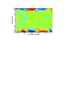
Figure 2.: The diagram latitude-time for Carrington rotations $1670-2190$ ($1978-2016$). The color scale represents the relative abundance of the positive and negative pixels at each latitude (red color corresponds to the presence only of positive pixels $B>0$ G, blue color corresponds to the presence only of negative pixels $B<0$ G).map

The 22-year periodicity in the magnetic field polarity is shown as alternation of blue and red regions near the poles. The middle points of the corresponding time intervals coincide with the SA minima. However the 11-year cycle of SA is hardly distinguishable in the sunspot zones because the contribution of the strong fields is suppressed. As a result the alternating blue-green and red-yellow inclined strips going from the equator to poles became clearly seen. Apparently, these strips correspond to streams of the magnetic fields of different polarities which are transferred to the poles due to the meridional circulation. The inclination of these strips (number of degrees/rotation) allows to evaluate the speed of the field transfer. The estimates give the following speed values: for the northern hemisphere $13.1\pm 0.8$ m/s and for southern (where separate streams are more pronounced) $12.9\pm 0.6$ m/s. These estimates are slightly lower than the value of speed 20 m/s obtained by measurement of Doppler shift (see Petrie, 2012 and references in it), however they lie within the limits of $10-20$ m/s observed by Roudier et al. (2018).

Most clearly appear in Figure map the near-polar regions where one of the two polarities alternately dominates defining the general dominating polarity of this hemisphere. In Figure hemalla time change of relative number of pixels with the positive polarity $N_{plus}$ is presented as a percentage for the northern hemisphere. It can be seen that the area occupied by the positive fields in the northern hemisphere is closely connected with the sign of the polar field in this hemisphere and changes with the 22-year period. During those periods of time when the sign of the northern polar field was positive, the area occupied by the positive polarity in SA minimum is up to $60\%$ of the hemisphere surface (Figure hemalla). Similar conclusions apply to the time changes of the negative field percentage, but the negative fields in the northern hemisphere develop in an antiphase with the fields of the positive polarity, reaching the maximum area when the sign of the northern polar field is negative. In Figure hemallb relative change in number of pixels with positive polarity $S_{plus}$ is presented as a percentage for the southern hemisphere. The same conclusions, as for the northern hemisphere are true: the positive polarity of the southern hemisphere is closely connected with the sign of the polar field in the southern hemisphere and reaches the maximum values $\sim 60\%$ in years close to the SA minimum. The dominating fields in each hemisphere during 11 years are those which sign coincides with the sign of the polar field in this hemisphere. Thus, the imbalance of positive and negative fields in each hemisphere changes with the 22-year period.

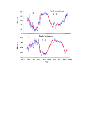
Figure 3.: The area of the Sun’s surface (as a percentage) occupied with magnetic fields (a) of positive polarity in the whole northern hemisphere $N_{plus}$ and (b) of positive polarity in the southern hemisphere $S_{plus}$ for each Carrington rotation. Red lines show the sliding smoothing on 20 rotations.hemall

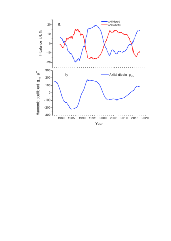
Figure 4.: (a) The imbalance of the number of positive and negative pixels as a percentage for the northern and southern hemispheres: $\Delta N(North)=N_{plus}-N_{minus}$ (blue line) and $\Delta N(South)=S_{plus}-S_{minus}$ (red line), respectively. (b) axial dipole moment $g_{10}$ of the magnetic field (WSO).g10

In Figure g10a imbalances of magnetic fields for the northern hemisphere $N_{plus}-N_{minus}$ and the southern hemisphere $S_{plus}-S_{minus}$ are presented. Though in this case we do not take into account the magnetic field strength B and consider the whole range of latitudes, we receive results close to those obtained in (Vernova et al., 2018) for high latitudes (from $40^{\circ}$ up to $90^{\circ}$) and the fields with $B<50$ G. Consequently the dipole magnetic field is the determining factor for the polarity imbalance in a separate hemisphere. In Figure g10b the axial dipole moment $g_{10}$ is shown which was calculated at the Wilcox Solar Observatory (WSO, http://wso.stanford.edu/) using PFSS model. The polarity imbalance in the northern hemisphere changes in phase with the dipole moment $g_{10}$ (Figure g10a,b).

Connection of the surface area occupied by the fields of a certain polarity with the sign of the polar field is most pronounced for the high-latitude fields (from $40^{\circ}$ to $90^{\circ}$). We compare positive fields of the northern hemisphere (Figure higha) and negative fields of the southern hemisphere (Figure highb). These fields develop in phase showing the correlation coefficient $R=0.94$. At high latitudes the fields of the positive polarity occupy about $80\%$ of the surface when the sign of the northern polar field is positive during SA minimum (Figure higha). If we consider the whole hemisphere, the percentage is about $60\%$ (see Figure hemalla). Two characteristic groups of the large-scale magnetic fields were described by Andryeyeva and Stepanian (2008): the first group represented weak background fields $3-10$ G, the second group represented stronger fields $75-100$  G. It was shown that weak fields with the N-polarity in the northern hemisphere correlate with the S-polarity fields in the southern hemisphere. This result is in good agreement with Figure high.

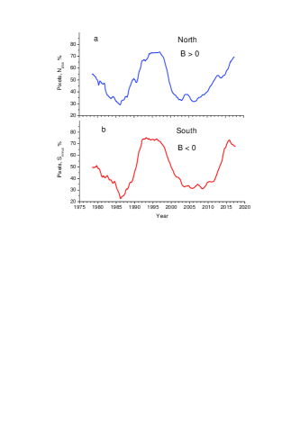
Figure 5.: High heliolatitudes. The area of the Sun’s surface (as a percentage) occupied with the magnetic fields (a) of positive polarity in the northern hemisphere $N_{plus}$ (heliolatitudes from $+40^{\circ}$ to $+90^{\circ}$) and (b) of negative polarity in the southern hemisphere $S_{minus}$ (from $-40^{\circ}$ to $-90^{\circ}$). Data are averaged over 20 solar rotations. high

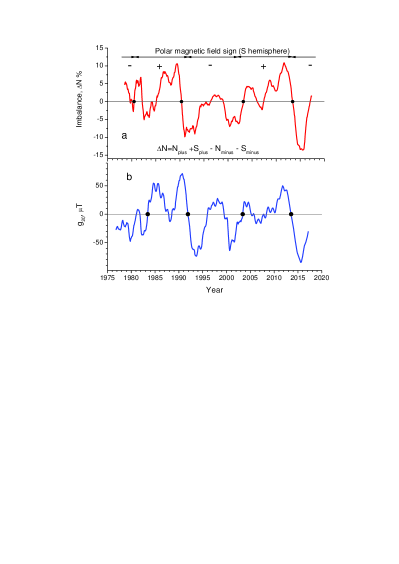
Figure 6.: The polarity imbalance at the high latitudes. (a) Heliolatitudes from $+40^{\circ}$ to $+90^{\circ}$ and from $-40^{\circ}$ to $-90^{\circ}$: the difference of number of positive and negative pixels in polar regions of two hemispheres ($\Delta N=N_{plus}+S_{plus}-N_{minus}-S_{minus}$). In the top part of the figure the sign of the polar field in the southern hemisphere is shown; (b) quadrupole moment $g_{20}$ of magnetic field (WSO). Black circles mark the sign changes of the imbalance near periods of the polar field reversal.imbhigh

To estimate the total polarity imbalance for high latitudes ($40^{\circ}-90^{\circ}$) we considered the difference of number of positive and negative pixels $\Delta N$ in polar regions of both hemispheres (Figure imbhigha):

$$\ilabel{dpix}\Delta N=N_{plus}+S_{plus}-N_{minus}-S_{minus}$$ (1)

During four solar cycles the strict regularity of the imbalance change is observed. For 11 years from one solar maximum to another the imbalance keeps the sign, changing it during the period close to the reversal of the polar field. Thus the periodicity of the imbalance-sign change is 22 years. The sign of the imbalance coincides with the sign of the polar field in the southern hemisphere (the sign is shown at the top of Figure imbhigha). In Figure imbhighb the quadrupole moment $g_{20}$ of the photospheric magnetic field (WSO) is shown. The polarity imbalance and the quadrupole moment have nearly the same time course, displaying good coincidence of their signs. These results agree with our conclusions in (Vernova et al., 2018) where the magnetic field strength was taken into account.

In the sunspot zone the positive and negative fields occupy approximately equal areas. Nevertheless in the latitude range from $-40^{\circ}$ to $+40^{\circ}$ some difference between the number of the positive and negative pixels is observed (Figure imblow, the blue line), the maximum of the imbalance being $5-8\%$ of the total number of pixels. The quadrupole moment taken with the reversed sign $-g_{20}$ is shown in Figure imblow (the red line). For several time periods both parameters change the sign almost simultaneously. The similarity of changes in the imbalance and the quadrupole moment is observed from 1978 to 2003 though the imbalance is a little shifted relative to the quadrupole moment. Discrepancy of these curves is seen at the decrease phase of Cycle 23 when the imbalance continues to remain positive (2003–2008) while the quadrupole moment $-g_{20}$ becomes negative. From 2009 to 2016 the imbalance and the quadrupole moment change almost synchronously.

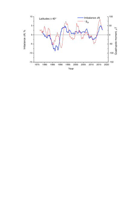
Figure 7.: The imbalance of the positive and negative pixel number at the equatorial latitudes $\pm 40^{\circ}$ - the blue line and the quadrupole moment with the reversed sign ($-g_{20}$)

- the red line. imblow

The recurrence of the imbalance is similar to the features of the imbalance of strong magnetic fields (Vernova et al., 2018). Change of the sign of the imbalance in the years close to reversals of the polar field was the main feature of the imbalance of the strong fields of the sunspot zone. The sign of the imbalance of the strong fields changes with the 22-year period just as the sign of the quadrupole moment $-g_{20}$ and coincides with the sign of the polar field in the northern hemisphere. The same features can be seen in Figure imblow in the imbalance of the positive and negative fields considered irrespective of the magnetic field strength. Thus, though not for the whole interval of time, there is a connection of the sign of the magnetic field imbalance of the sunspot zone with the quadrupole moment $-g_{20}$ and with the sign of the polar field in the northern hemisphere. The time interval when the sign of the imbalance and the sign of the quadrupole moment coincide is about $75\%$ of the considered period of time.

4 Conclusions

1. We consider distribution of the positive and negative magnetic fields over the surface of the Sun for four solar cycles, taking into account only the field sign irrespective of its strength. Such approach allows us to emphasize the peculiarities of the distribution of the magnetic fields with average and small strengths due to the suppression of the strong fields connected with active regions of the Sun. Thus, we study the area occupied with fields of the positive and negative polarities.

2. We show that the features of the distribution for the fields of different polarity are defined generally by the high-latitude fields. The polarity imbalance in each hemisphere is closely connected with the changes in the dipole moment $g_{10}$. The effect of the dipole component of the field on the imbalance of the positive and negative fields is observed for the whole hemisphere, and not just for high latitudes, as it was in the case when the magnetic field strength was taken into account.

3. For high latitudes the imbalance of positive and negative fields in the latitude ranges from $+40^{\circ}$ to $+90^{\circ}$ and from $-40^{\circ}$ to $-90^{\circ}$ is considered. The sign of the imbalance changes with the 22-year period and coincides both with the sign of the polar field in the southern hemisphere, and with the sign of the quadrupole moment $g_{20}$. These important results are obtained by taking into account only the area occupied by the fields of positive or negative polarities.

4. For the most part of time ($\sim 75\%$) for the fields in the latitude range $\pm 40^{\circ}$ we observe coincidence of the imbalance sign of magnetic fields with the reversed sign of quadrupole moment $-g_{20}$ and with the sign of the polar field in the northern hemisphere.

5. The diagram latitude-time shows structures in the form of inclined strips which became discernible due to the domination of one of the polarities. The inclination of these strips, apparently, is connected with transfer of magnetic fields in the direction from the equator to the poles. In that case the speed of transfer will be equal to about 13 m/s which is close to estimates of speed of meridional circulation made by the other authors.

5 Acknowledgements

NSO/Kitt Peak data used here are produced cooperatively by NSF/NOAO, NASA/GSFC, and NOAA/SEL. This work utilizes SOLIS data obtained by the NSO Integrated Synoptic Program (NISP), managed by the National SolarObservatory. Wilcox Solar Observatory data used in this study was obtained via the web site http://wso.stanford.edu courtesy of J.T. Hoeksema.

References

- Akhtemov et al. (2015) Akhtemov, Z.S., Andreyeva, O.A., Rudenko, G.V., Stepanian, N.N., and Fainshtein, V.G.: 2015, Adv. Space Res. 55, 3, 968. ADS, DOI.
- Andryeyeva and Stepanian (2008) Andryeyeva, O.A., Stepanian, N.N.: 2008, Astron. Nachr. 329, 579. ADS, DOI.
- Bravo and González-Esparza (2000) Bravo, S., González-Esparza, J.A.: 2000, Geophys. Res. Lett. 27, 847. ADS, DOI.
- Charbonneau (2010) Charbonneau, P.: 2010, Living Rev. Solar Phys. 7, 3. ADS, DOI.
- Hoeksema (1991) Hoeksema, J.T.: 1991, J. Geomagn. Geoelectr. 43, Suppl., 59.
- Hoeksema and Scherrer (1986) Hoeksema, J.T., Scherrer, P.H.: 1986, Solar Magnetic Field – 1976 through 1985. Report UAG-94, WDCA, Boulder, USA. ADS.
- Ioshpa, Obridko, and Chertoprud (2009) Ioshpa, B.A.; Obridko, V.N.; Chertoprud, V.E.: 2009, Astron. Let. 35, 424. ADS, DOI.
- Kotov (2009) Kotov, V.A.: 2009, Bull. Crimean Astrophys. Obs. 105, 45. ADS, DOI.
- Petrie (2012) Petrie, G.J.D.: 2012, Solar Phys. 289, 577. ADS, DOI.
- Roudier et al. (2018) Roudier, Th., Švanda, M., Ballot, J., Malherbe, J.M., Rieutord, M.: 2018, Astron. Astrophys. 611, id.A92, 9pp. ADS, DOI.
- Svalgaard and Kamide (2013) Svalgaard, L., Kamide, Y.: 2013, Astrophys. J. 763, 23. ADS, DOI.
- Vernova et al. (2018) Vernova, E.S., Tyasto, M.I., Baranov, D.G., Danilova, O.A.: 2018, Solar Phys. 293, 158. ADS, DOI.
- Wilcox (1972) Wilcox, J.M.: 1972, Comments Astrophys. Space Phys. 4, 141. ADS.