Study of warm inflationary models and their parameter estimation from CMB

Richa Arya    Raghavan Rangarajan
Abstract

Observations of the temperature anisotropies in the Cosmic Microwave Background (CMB) radiation show that the models of inflation with the monomial potentials are inconsistent with the allowed nsrsubscript𝑛𝑠𝑟n_{s}-r bounds. However certain monomial potentials of inflation are allowed in the context of Warm Inflation, where the inflaton’s coupling with other fields are significant both during and after the inflationary phase. In our study, we consider λϕ4𝜆superscriptitalic-ϕ4\lambda\phi^{4} and λϕ6𝜆superscriptitalic-ϕ6\lambda\phi^{6} models of warm inflation with different forms of the inflaton dissipation coefficient. We parameterize the primordial power spectrum in terms of the model parameters, namely, the inflaton self coupling, λ𝜆\lambda, and the dissipation parameter, QPsubscript𝑄𝑃Q_{P}, due to inflaton’s interaction with the other fields. Then we obtain the joint and marginal distributions of these parameters by carrying out a Markov Chain Monte Carlo (MCMC) analysis using the CosmoMC numerical code. An estimation of these physical parameters is essential for model building. We also obtain the nssubscript𝑛𝑠n_{s} and r𝑟r values for the mean values of the parameters and find them to be consistent with the observational bounds, confirming that these simple models are viable models for describing inflation.

1 Introduction

Cosmological Inflation [1, 2, 3, 4, 5, 6, 7] is a phase of accelerated expansion for a very brief duration in the early Universe. It provides a solution to many shortcomings of the Standard Big Bang Model of cosmology. As a bonus, it also provides a mechanism to generate the primordial density fluctuations that can explain the anisotropies in the Cosmic Microwave Background (CMB) radiation and seed the growth of Large Scale Structure (LSS) at late times. (For a review, refer to Refs. [8, 9].)

Inflation is driven by a scalar field, ϕitalic-ϕ\phi, known as the inflaton. When the energy density of the inflaton field dominates the energy density of the Universe, inflation takes place. In the standard description, one presumes that the inflaton’s coupling to other fields are ineffective during the slow roll inflationary phase. During inflation, the Universe expands nearly exponentially and consequently, the number densities of all species dilute away and the Universe enters into a supercooled state. When inflation ends, the Universe undergoes a reheating phase in which the inflaton oscillates and dissipates its energy into particles [10]. We refer to this inflationary scenario as Cold Inflation.

However, there is another description of inflation known as Warm Inflation [11, 12, 13], in which one considers the inflaton’s coupling with other fields both during and after inflation. As the inflaton dissipates into radiation during the slow roll inflationary phase as well, the Universe is not supercooled and has a temperature and is hence warm during inflation (for a review refer to Refs. [14, 15]). The condition for warm inflation to take place is that the temperature of the thermal bath of radiation should be greater than the Hubble expansion of the Universe (T>H𝑇𝐻T>H), so that the thermal de Broglie wavelength of the radiation (T1proportional-toabsentsuperscript𝑇1\propto T^{-1}) is smaller than the Hubble radius (H1superscript𝐻1H^{-1}).

The importance of studying warm inflation are manifold. First, it is natural and proper to include the inflaton couplings to other fields not just in the reheating phase, but also during the inflationary phase. Second, the condition of the flat potential required for the slow roll of inflaton is somewhat relaxed in warm inflation. As a result inflation can last long enough even if the potential is not very flat. Third, as pointed out in Refs. [16, 17, 18, 19], certain monomial potentials of inflation are viable models in warm inflation, unlike in cold inflation where they are ruled out. Therefore it is crucial to reconsider the monomial models in warm inflation and constrain their parameters using the CMB observations.

In our previous work [20], we obtained the model parameters for a λϕ4𝜆superscriptitalic-ϕ4\lambda\phi^{4} potential model of warm inflation with a cubic dissipation coefficient. In this study, we consider a λϕ4𝜆superscriptitalic-ϕ4\lambda\phi^{4} potential with a linear dissipation coefficient and a λϕ6𝜆superscriptitalic-ϕ6\lambda\phi^{6} potential with linear and cubic dissipation coefficients and carry out a Markov Chain Monte Carlo (MCMC) analysis to obtain the parameters consistent with the CMB observations. We parameterize the primordial power spectrum for our models in terms of two parameters, namely, λ𝜆\lambda, representing the inflaton self coupling, and the dissipation parameter at the pivot scale, QPsubscript𝑄𝑃Q_{P}, due to the inflaton’s interactions with other fields, and obtain their mean values. This is crucial for model building. We also verify that the nssubscript𝑛𝑠n_{s} and r𝑟r values for these mean values are compatible with the observational data.

Warm inflationary models usually require coupling the inflaton to a very large number of fields to maintain T>H𝑇𝐻T>H [16, 21]. Such a large number of fields can be achieved through some string theory inspired generation mechanism [22]. However recently proposed warm inflation models with the inflaton as a pseudo-Nambu-Goldstone boson require very few additional fields [23, 24] and allow for a well-motivated particle physics description.

The objective of our work is to study scalar field monomial potentials in the context of warm inflation and estimate the parameters that are consistent with the observations using a publicly available numerical code named CosmoMC [25]. We use the Planck 2015 data (high-l TT, TE, TE + low-l polarization) for our analysis. We plot the joint probability distribution of our model parameters and list the marginalised values of all the parameters along with 68%percent6868\% C.L. values using the GetDist GUI software.

This paper is organised as follows. We first overview the basic evolution equations for the inflaton and the radiation fields and define the slow roll parameters and conditions in Section 2. We also state the conditions required for warm inflation to begin and to end. We describe the primordial power spectrum for warm inflation and the forms of the dissipation coefficient that we consider. In Section 3, we present the models that we consider. Then in Sections 4, 5, 6, we parameterize the primordial power spectrum for our models in terms of the model parameters, λ𝜆\lambda, and QPsubscript𝑄𝑃Q_{P}. In Section 7, we determine the scale dependence of the power spectrum. Then in Section 8, we do a preliminary analysis using Mathematica and plot the dependences of the model parameters. After that, we carry out a MCMC analysis using CosmoMC and obtain the mean values for the parameters for the different models in Section 9. We also list the values of nssubscript𝑛𝑠n_{s} and r𝑟r for the mean values of the parameters. Lastly we end with our conclusions in Section 10.

In our notation, overdot represents derivative w.r.t. time and prime represents derivative w.r.t. ϕitalic-ϕ\phi throughout this paper.

2 The theory of warm inflation

2.1 Evolution equations for the inflaton and radiation

The equation of motion of the homogeneous inflaton field ϕitalic-ϕ\phi during warm inflation is given as

ϕ¨+(3H+Υ)ϕ˙+V(ϕ)=0,¨italic-ϕ3𝐻Υ˙italic-ϕsuperscript𝑉italic-ϕ0\ddot{\phi}+(3H+\Upsilon)\dot{\phi}+V^{\prime}(\phi)=0\,, (2.1)

where H𝐻H is the Hubble expansion rate, and Υ(ϕ,T)Υitalic-ϕ𝑇\Upsilon(\phi,T) is the dissipation coefficient which is a measure of inflaton dissipation into radiation. In the literature there are many forms of Υ(ϕ,T)Υitalic-ϕ𝑇\Upsilon(\phi,T), which depend on the mechanism by which the inflaton dissipation takes place. In this study, we have considered temperature dependent forms of ΥΥ\Upsilon which are described in Section 2.4. The dissipative term Υϕ˙Υ˙italic-ϕ\Upsilon\dot{\phi} is absent in the cold inflation scenario.

As a result of the inflaton dissipation, radiation is concurrently produced during warm inflation. From the continuity equation, the energy density of radiation ρrsubscript𝜌𝑟\rho_{r} evolves as

ρ˙r+4Hρr=Υϕ˙2.subscript˙𝜌𝑟4𝐻subscript𝜌𝑟Υsuperscript˙italic-ϕ2\dot{\rho}_{r}+4H\rho_{r}=\Upsilon{\dot{\phi}}^{2}~{}. (2.2)

The energy dissipated by the inflaton, Υϕ˙2Υsuperscript˙italic-ϕ2\Upsilon{\dot{\phi}}^{2}, is transferred to radiation. We define a dissipation parameter

QΥ3H𝑄Υ3𝐻Q\equiv\frac{\Upsilon}{3H}

and rewrite Eq. (2.1) as

ϕ¨+3H(1+Q)ϕ˙+V(ϕ)=0.¨italic-ϕ3𝐻1𝑄˙italic-ϕsuperscript𝑉italic-ϕ0\ddot{\phi}+3H(1+Q)\dot{\phi}+V^{\prime}(\phi)=0. (2.3)

The dissipation parameter, Q𝑄Q, is the ratio of the strength of inflaton dissipation into radiation to the Hubble rate of expansion. For Q1much-greater-than𝑄1Q\gg 1, the dissipation coefficient is larger than H𝐻H, and this regime is termed as the strong dissipative regime. For Q1much-less-than𝑄1Q\ll 1, the expansion is faster than dissipation, and this is termed as the weak dissipative regime of warm inflation. In this study, we have considered both the regimes for our models.

2.2 Slow roll parameters and conditions

The flatness of the potential V(ϕ)𝑉italic-ϕV(\phi) in warm inflation is measured in terms of the slow roll parameters which are defined in Ref. [26] as

ϵϕ=MPl216π(V,ϕV)2,ηϕ=MPl28πV,ϕϕV,\epsilon_{\phi}=\frac{M_{Pl}^{2}}{16\pi}\,\left(\frac{V_{,\phi}}{V}\right)^{2},\hskip 28.45274pt\eta_{\phi}=\frac{M_{Pl}^{2}}{8\pi}\,\frac{V_{,\phi\phi}}{V},
βΥ=MPl28π(Υ,ϕV,ϕΥV),δ=TV,ϕTV,ϕ\beta_{\Upsilon}=\frac{M_{Pl}^{2}}{8\pi}\,\left(\frac{\Upsilon_{,\phi}\,V_{,\phi}}{\Upsilon\,V}\right),\hskip 28.45274pt\delta=\frac{TV_{,{\phi T}}}{V_{,\phi}} (2.4)

Here V,ϕV_{,\phi} is the derivative of V𝑉V w.r.t. ϕitalic-ϕ\phi and Υ,ϕ\Upsilon_{,\phi} is the derivative of ΥΥ\Upsilon w.r.t. ϕitalic-ϕ\phi. MPl=1GN=1.2×10¹⁹subscript𝑀𝑃𝑙1subscript𝐺𝑁1.2superscript1019M_{Pl}=\frac{1}{\sqrt{G_{N}}}=1.2\times 10^{19} GeV is the Planck mass. In cold inflation, there is no βΥsubscript𝛽Υ\beta_{\Upsilon} or δ𝛿\delta, as there is no dissipation and temperature during inflation. In the literature one also defines the horizon flow parameters as

ϵH=H˙H2,ηH=H¨2HH˙.formulae-sequencesubscriptitalic-ϵ𝐻˙𝐻superscript𝐻2subscript𝜂𝐻¨𝐻2𝐻˙𝐻\epsilon_{H}=\frac{-\dot{H}}{H^{2}},\qquad\quad\eta_{H}=\frac{-\ddot{H}}{2H\dot{H}}. (2.5)

These different definition of slow roll parameters are then related as

ϵH=ϵϕ1+Q,ηH=ηϕ1+Q.formulae-sequencesubscriptitalic-ϵ𝐻subscriptitalic-ϵitalic-ϕ1𝑄subscript𝜂𝐻subscript𝜂italic-ϕ1𝑄\epsilon_{H}=\frac{\epsilon_{\phi}}{1+Q},\qquad\eta_{H}=\frac{\eta_{\phi}}{1+Q}\,. (2.6)

The slow roll conditions needed for the warm inflationary phase are given in Ref. [27] as

ϵϕ1+Q,|ηϕ|1+Q,|βΥ|1+Q,0<δQ1+Q.formulae-sequencemuch-less-thansubscriptitalic-ϵitalic-ϕ1𝑄formulae-sequencemuch-less-thansubscript𝜂italic-ϕ1𝑄formulae-sequencemuch-less-thansubscript𝛽Υ1𝑄0𝛿much-less-than𝑄1𝑄\epsilon_{\phi}\ll 1+Q,\quad|\eta_{\phi}|\ll 1+Q,\quad|\beta_{\Upsilon}|\ll 1+Q,\quad 0<\delta\ll\frac{Q}{1+Q}. (2.7)

We can see that for significant Q𝑄Q, these conditions reduce the requirement for the potential to be extremely flat. In the slow roll approximation, we can neglect ϕ¨¨italic-ϕ\ddot{\phi} in Eq. (2.3) which gives

ϕ˙V(ϕ)3H(1+Q).˙italic-ϕsuperscript𝑉italic-ϕ3𝐻1𝑄\dot{\phi}\approx\frac{-V^{\prime}(\phi)}{3H(1+Q)}. (2.8)

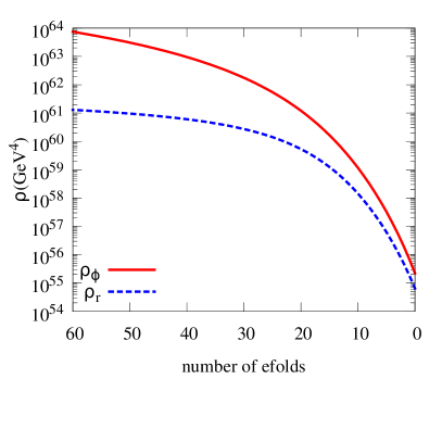
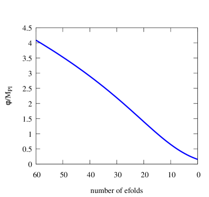
As shown in Fig. 1, the energy density of radiation does not change appreciably when the modes of cosmological interest cross the horizon. Also, ρ˙rsubscript˙𝜌𝑟\dot{\rho}_{r} is smaller than the other terms in Eq. (2.2) throughout inflation. Therefore, we can approximate ρ˙r0subscript˙𝜌𝑟0\dot{\rho}_{r}\approx 0 and obtain

ρr=π230gT4AT4Υ4Hϕ˙2=34Qϕ˙2,subscript𝜌𝑟superscript𝜋230subscript𝑔superscript𝑇4𝐴superscript𝑇4Υ4𝐻superscript˙italic-ϕ234𝑄superscript˙italic-ϕ2\rho_{r}=\frac{\pi^{2}}{30}g_{*}T^{4}\equiv AT^{4}\approx\frac{\Upsilon}{4H}{\dot{\phi}}^{2}=\frac{3}{4}Q{\dot{\phi}}^{2}, (2.9)

where gsubscript𝑔g_{*} is the number of relativistic degrees of freedom during warm inflation and we define A=π2g/30𝐴superscript𝜋2subscript𝑔30A=\pi^{2}g_{*}/30. (Here we take g200subscript𝑔200g_{*}\approx 200.)

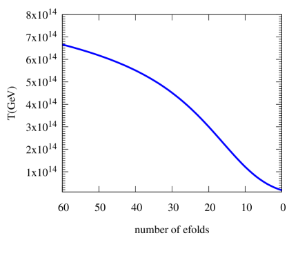
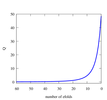
We show the behaviour of the evolution of ϕitalic-ϕ\phi (in units of MPlsubscript𝑀𝑃𝑙M_{Pl}) and the temperature T𝑇T during warm inflation for one of our models in Fig. 1. The dissipation parameter, Q𝑄Q, depends on both ϕitalic-ϕ\phi and T𝑇T, and is not a constant but rather evolves during inflation. This behaviour can also be seen in Fig. 1. It is possible that inflation starts in the weak dissipation regime, and with the evolution of Q𝑄Q, ends in the strong dissipation regime.

As already mentioned, the notion of a temperature is only valid for T>H𝑇𝐻T>H. For the models we have considered, we find that T>H𝑇𝐻T>H at all times during inflation holds for QP>105subscript𝑄𝑃superscript105Q_{P}>10^{-5}. So we have a lower bound on the value of QPsubscript𝑄𝑃Q_{P} of 105superscript10510^{-5}.

2.3 End of warm inflation

In the standard cold inflation, the violation of slow roll conditions marks the end of inflation. But warm inflation ends when either the slow roll conditions are violated or the radiation energy density dominates the inflaton energy density, i.e. ρr>ρϕ.subscript𝜌𝑟subscript𝜌italic-ϕ\rho_{r}>\rho_{\phi}. In Fig. 1, we plot the radiation and inflaton energy density as a function of N,𝑁N, the number of efolds from the end of inflation. For our models ρϕsubscript𝜌italic-ϕ\rho_{\phi} is larger than ρrsubscript𝜌𝑟\rho_{r}, even when the slow roll conditions fail and therefore the end of inflation is governed by the breaking of the slow roll conditions. As a consequence, the Universe will also go through a phase of reheating after inflation for the models we have considered.
Refer to caption
Refer to caption
Refer to caption
Refer to caption
Figure 1: The behaviour of the homogeneous inflaton field ϕitalic-ϕ\phi (in units of MPlsubscript𝑀𝑃𝑙M_{Pl}), the dissipation parameter Q𝑄Q, the energy density in ϕitalic-ϕ\phi (red solid) and radiation (blue dashed), and temperature T𝑇T of the Universe is shown as a function of the number of efolds N𝑁N counted from the end of inflation for V(ϕ)=λϕ6MPl2𝑉italic-ϕ𝜆superscriptitalic-ϕ6superscriptsubscript𝑀𝑃𝑙2V(\phi)=\lambda\frac{\phi^{6}}{M_{Pl}^{2}} with the dissipation coefficient Υ=CTTΥsubscript𝐶𝑇𝑇\Upsilon=C_{T}T. To generate this plot, we take QP=0.1subscript𝑄𝑃0.1Q_{P}=0.1, and as will be described later, fix the normalisation of the primordial power spectrum at the pivot scale P(kP)As=2.2×10⁹subscript𝑃subscript𝑘𝑃subscript𝐴𝑠2.2superscript109P_{\mathcal{R}}(k_{P})\equiv A_{s}=2.2\times 10^{-9}, and set NP=60subscript𝑁𝑃60N_{P}=60. This behaviour is similar for all the models we have considered.

2.4 Different forms of the dissipation coefficient considered

In the literature, a general expression for the dissipation coefficient is given as

Υ(ϕ,T)=CTcϕ2a/MX2bΥitalic-ϕ𝑇𝐶superscript𝑇𝑐superscriptitalic-ϕ2𝑎superscriptsubscript𝑀𝑋2𝑏\Upsilon(\phi,T)=CT^{c}\phi^{2a}/M_{X}^{2b} (2.10)

with a condition c+2a2b=1𝑐2𝑎2𝑏1c+2a-2b=1 [28], where MXsubscript𝑀𝑋M_{X} is the mass of the fields X𝑋X which are coupled to the inflaton. Here we have considered the following two forms of the dissipation coefficient for the supersymmetric models of inflation in which the inflaton is coupled with the intermediate bosonic and fermionic components of a superfield, X𝑋X, which subsequently decay into the scalar and fermionic components of the superfield, Y𝑌Y [29]. The field Y𝑌Y with mYTmuch-less-thansubscript𝑚𝑌𝑇m_{Y}\ll T thermalise and constitute the thermal bath.

  1. 1.

    Dissipation coefficient with a cubic dependence on the temperature,

    Υ(ϕ,T)=CϕT3ϕ2.Υitalic-ϕ𝑇subscript𝐶italic-ϕsuperscript𝑇3superscriptitalic-ϕ2\Upsilon(\phi,T)=C_{\phi}\frac{T^{3}}{\phi^{2}}. (2.11)

    This kind of dissipation term arises in the low temperature regime of warm inflation, where the intermediate X𝑋X fields are heavy (mXTmuch-greater-thansubscript𝑚𝑋𝑇m_{X}\gg T) [29, 30, 31]. The dimensionless constant Cϕsubscript𝐶italic-ϕC_{\phi} depends on the couplings and the multiplicities of X𝑋X and Y𝑌Y and is defined as

    Cϕ=14αNXsubscript𝐶italic-ϕ14𝛼subscript𝑁𝑋C_{\phi}=\frac{1}{4}\alpha N_{X}

    where α=h2NY4π𝛼superscript2subscript𝑁𝑌4𝜋\alpha=h^{2}\frac{N_{Y}}{4\pi} is less than 111, hh is the coupling between ϕitalic-ϕ\phi and X𝑋X, and NX,Ysubscript𝑁𝑋𝑌N_{X,Y} are the multiplicities of the X𝑋X and Y𝑌Y fields [32]. NXsubscript𝑁𝑋N_{X} can be very large; for example, for the sextic potential model that we consider with a cubic dissipation coefficient, Cϕsubscript𝐶italic-ϕC_{\phi} is 4×1074superscript1074\times 10^{7} for the mean values of the model parameters and so assuming α=0.1𝛼0.1\alpha=0.1, we get NX109similar-tosubscript𝑁𝑋superscript109N_{X}\sim 10^{9}. Such a huge number of fields is a drawback for the warm inflationary models.

  2. 2.

    Dissipation coefficient with a linear dependence on temperature,

    Υ(ϕ,T)=CTT.Υitalic-ϕ𝑇subscript𝐶𝑇𝑇\Upsilon(\phi,T)=C_{T}T. (2.12)

    This kind of dissipation term arises in the high temperature regime of warm inflation, where the X𝑋X fields are light, TmXmuch-greater-than𝑇subscript𝑚𝑋T\gg m_{X} [29, 30].

2.5 Primordial power spectrum

The primordial power spectrum for the warm inflation is given in Refs. [32, 24, 19, 28] (based on the references therein) as

P(k)=(Hk22πϕ˙k)2[1+2nk+(TkHk)23πQk3+4πQk]G(Qk),subscript𝑃𝑘superscriptsuperscriptsubscript𝐻𝑘22𝜋subscript˙italic-ϕ𝑘2delimited-[]12subscript𝑛𝑘subscript𝑇𝑘subscript𝐻𝑘23𝜋subscript𝑄𝑘34𝜋subscript𝑄𝑘𝐺subscript𝑄𝑘P_{\mathcal{R}}(k)=\left(\frac{H_{k}^{2}}{2\pi\dot{\phi}_{k}}\right)^{2}\left[1+2n_{k}+\left(\frac{T_{k}}{H_{k}}\right)\frac{2\sqrt{3}\pi Q_{k}}{\sqrt{3+4\pi Q_{k}}}\right]G(Q_{k}), (2.13)

where the subscript k𝑘k signifies the time when the mode of cosmological perturbations with wavenumber k𝑘k leaves the horizon during inflation, and the inflaton distribution nksubscript𝑛𝑘n_{k} is taken as a Bose-Einstein distribution,

nk=1exp(k/akTk)1subscript𝑛𝑘1𝑘subscript𝑎𝑘subscript𝑇𝑘1n_{k}=\frac{1}{\exp(\frac{k/a_{k}}{T_{k}})-1}

where a𝑎a is the scale factor and T𝑇T represents the physical temperature. Then

1+2nk=cothHk2Tk.12subscript𝑛𝑘hyperbolic-cotangentsubscript𝐻𝑘2subscript𝑇𝑘1+2n_{k}=\coth\frac{H_{k}}{2T_{k}}.

The perturbations in the radiation, because of inhomogeneous dissipation, can lead to growing inflaton perturbations in the primordial power spectrum [33]. This growth factor G(Qk)𝐺subscript𝑄𝑘G(Q_{k}) is dependent on the form of ΥΥ\Upsilon and is obtained numerically. As given in Ref. [24, 19]

ForΥTG(Qk)linear=1+0.0185Qk2.315+0.335Qk1.364formulae-sequenceproportional-toForΥ𝑇𝐺subscriptsubscript𝑄𝑘𝑙𝑖𝑛𝑒𝑎𝑟10.0185superscriptsubscript𝑄𝑘2.3150.335superscriptsubscript𝑄𝑘1.364{\rm For\,\,}\Upsilon\propto T\qquad\qquad G(Q_{k})_{linear}=1+0.0185\,Q_{k}^{2.315}+0.335\,Q_{k}^{1.364}
ForΥT3G(Qk)cubic=1+4.981Qk1.946+0.127Qk4.330.formulae-sequenceproportional-toForΥsuperscript𝑇3𝐺subscriptsubscript𝑄𝑘𝑐𝑢𝑏𝑖𝑐14.981superscriptsubscript𝑄𝑘1.9460.127superscriptsubscript𝑄𝑘4.330{\rm For\,\,}\Upsilon\propto T^{3}\qquad\qquad G(Q_{k})_{cubic}=1+4.981\,Q_{k}^{1.946}+0.127\,Q_{k}^{4.330}.

In the weak dissipation regime for small Q𝑄Q, the growth factor does not enhance the power spectrum much. But for Q>1𝑄1Q>1 in the strong dissipation regime, the growth factor significantly enhances the power spectrum.

The primordial tensor fluctuations of the metric give rise to a tensor power spectrum given in Ref. [32] as

PT(k)=16π(HkMPl)2.subscript𝑃𝑇𝑘16𝜋superscriptsubscript𝐻𝑘subscript𝑀𝑃𝑙2P_{T}(k)=\frac{16}{\pi}\left(\frac{H_{k}}{M_{Pl}}\right)^{2}. (2.14)

The ratio of the tensor to the scalar power spectrum is expressed in terms of a parameter r𝑟r as

r=PT(k)P(k).𝑟subscript𝑃𝑇𝑘subscript𝑃𝑘r=\frac{P_{T}(k)}{P_{\mathcal{R}}(k)}. (2.15)

3 Models of warm inflation considered

With the recent measurements of the temperature anisotropies in the Cosmic Microwave Background (CMB) radiation, tighter constraints on the spectral index of scalar perturbations, nssubscript𝑛𝑠n_{s} and the tensor-to-scalar ratio, r𝑟r are obtained which rule out simple monomial potential models of inflation like V(ϕ)=λϕ4𝑉italic-ϕ𝜆superscriptitalic-ϕ4V(\phi)=\lambda\phi^{4} and V(ϕ)=λϕ6𝑉italic-ϕ𝜆superscriptitalic-ϕ6V(\phi)=\lambda\phi^{6}. In our earlier work, we obtained the parameters of warm inflation for a potential, V(ϕ)=λϕ4𝑉italic-ϕ𝜆superscriptitalic-ϕ4V(\phi)=\lambda\phi^{4}, with a cubic dissipation coefficient Υ=CϕT3ϕ2Υsubscript𝐶italic-ϕsuperscript𝑇3superscriptitalic-ϕ2\Upsilon=C_{\phi}\frac{T^{3}}{\phi^{2}} in the weak dissipative regime [20]. For the strong dissipative regime, the nssubscript𝑛𝑠n_{s} and r𝑟r values were out of the Planck 2015 allowed values and hence this case is not of interest. Here in this study, we have considered the following models in the weak and strong dissipative regimes.

  • Model I: V(ϕ)=λϕ4𝑉italic-ϕ𝜆superscriptitalic-ϕ4V(\phi)=\lambda\phi^{4} with the dissipation coefficient Υ=CTTΥsubscript𝐶𝑇𝑇\Upsilon=C_{T}T.

  • Model II: V(ϕ)=λϕ6MPl2𝑉italic-ϕ𝜆superscriptitalic-ϕ6superscriptsubscript𝑀𝑃𝑙2V(\phi)=\lambda\frac{\phi^{6}}{M_{Pl}^{2}} with the dissipation coefficient Υ=CTTΥsubscript𝐶𝑇𝑇\Upsilon=C_{T}T.

  • Model III: V(ϕ)=λϕ6MPl2𝑉italic-ϕ𝜆superscriptitalic-ϕ6superscriptsubscript𝑀𝑃𝑙2V(\phi)=\lambda\frac{\phi^{6}}{M_{Pl}^{2}} with the dissipation coefficient Υ=CϕT3ϕ2Υsubscript𝐶italic-ϕsuperscript𝑇3superscriptitalic-ϕ2\Upsilon=C_{\phi}\frac{T^{3}}{\phi^{2}}.

For all the models, we first parametrize the primordial power spectrum in terms of the model parameters. After a primary analysis of the models with Mathematica, we perform a detailed Markov Chain analysis with CosmoMC and present the mean values of the parameters along with the 68%percent6868\% confidence limits. Then for the mean values we compute nssubscript𝑛𝑠n_{s} and r𝑟r and compare their values with the Planck 2015 results.

4 Primordial power spectrum for V(ϕ)=λϕ4𝑉italic-ϕ𝜆superscriptitalic-ϕ4V(\phi)=\lambda\phi^{4} with Υ=CTTΥsubscript𝐶𝑇𝑇\Upsilon=C_{T}T

In this section, we evaluate each factor of the primordial power spectrum Psubscript𝑃P_{\mathcal{R}} given in Eq. (2.13), and express them in terms of the inflaton self coupling λ𝜆\lambda, dissipation parameter Q𝑄Q, and the dimensionless constant CTsubscript𝐶𝑇C_{T}. In Section 7, we shall obtain Q(k)𝑄𝑘Q(k) which thereby gives Psubscript𝑃P_{\mathcal{R}} as a function of k𝑘k, λ𝜆\lambda and CTsubscript𝐶𝑇C_{T}. We will see in Section 7.3 that with another constraint on the number of efolds, the parameters λ𝜆\lambda and CTsubscript𝐶𝑇C_{T} are related. Then we will have only two independent model parameters, λ𝜆\lambda and QPsubscript𝑄𝑃Q_{P}, for CosmoMC111This model was also considered in Ref. [34], however, the power spectrum was parameterized differently..

  1. 1.

    The prefactor: The energy density during inflation is predominantly the potential of the inflaton field. Therefore we can write the Einstein equation as

    H2=8π3λϕ4MPl2.superscript𝐻28𝜋3𝜆superscriptitalic-ϕ4superscriptsubscript𝑀𝑃𝑙2H^{2}=\frac{8\pi}{3}\frac{\lambda\phi^{4}}{M_{Pl}^{2}}. (4.1)

    Using this we can express Eq. (2.8) for this model as

    ϕ˙V(ϕ)3H(1+Q)=4338πλϕMPl(1+Q).˙italic-ϕsuperscript𝑉italic-ϕ3𝐻1𝑄4338𝜋𝜆italic-ϕsubscript𝑀𝑃𝑙1𝑄\dot{\phi}\approx\frac{-V^{\prime}(\phi)}{3H(1+Q)}=-\frac{4}{3}\sqrt{\frac{3}{8\pi}}\sqrt{\lambda}\frac{\phi M_{Pl}}{(1+Q)}. (4.2)

    Then combining these, we can write 222The minus sign on the rhs was missed in Ref. [20] but it does not affect the power spectrum.

    Hk22πϕ˙k=8π3λ(ϕkMPl)3(1+Qk).superscriptsubscript𝐻𝑘22𝜋subscript˙italic-ϕ𝑘8𝜋3𝜆superscriptsubscriptitalic-ϕ𝑘subscript𝑀𝑃𝑙31subscript𝑄𝑘\frac{H_{k}^{2}}{2\pi\dot{\phi}_{k}}=-\sqrt{\frac{8\pi}{3}}\sqrt{\lambda}\left(\frac{\phi_{k}}{M_{Pl}}\right)^{3}(1+Q_{k}). (4.3)
  2. 2.

    T/H factor: On substituting Eq. (4.2) in the energy density of radiation given in Eq. (2.9), we obtain the temperature of the thermal bath as

    Tk=(15π3gQk(1+Qk)2λϕk2MPl2)14subscript𝑇𝑘superscript15superscript𝜋3subscript𝑔subscript𝑄𝑘superscript1subscript𝑄𝑘2𝜆superscriptsubscriptitalic-ϕ𝑘2superscriptsubscript𝑀𝑃𝑙214T_{k}=\left(\frac{15}{\pi^{3}g_{*}}\frac{Q_{k}}{(1+Q_{k})^{2}}\lambda\,\phi_{k}^{2}M_{Pl}^{2}\right)^{\frac{1}{4}} (4.4)

    and then combining with H𝐻H from Eq. (4.1), the factor T/H𝑇𝐻T/H becomes

    TkHk=(15π3g)1438πλ14Qk14(1+Qk)12(ϕkMPl)3/2.subscript𝑇𝑘subscript𝐻𝑘superscript15superscript𝜋3subscript𝑔1438𝜋superscript𝜆14superscriptsubscript𝑄𝑘14superscript1subscript𝑄𝑘12superscriptsubscriptitalic-ϕ𝑘subscript𝑀𝑃𝑙32\frac{T_{k}}{H_{k}}=\left(\frac{15}{\pi^{3}g_{*}}\right)^{\frac{1}{4}}\sqrt{\frac{3}{8\pi}}\lambda^{-\frac{1}{4}}\frac{Q_{k}^{\frac{1}{4}}}{(1+Q_{k})^{\frac{1}{2}}}\left(\frac{\phi_{k}}{M_{Pl}}\right)^{-3/2}. (4.5)

The dissipation parameter is defined as Q=Υ3H𝑄Υ3𝐻Q=\frac{\Upsilon}{3H}. In this model of warm inflation, we have considered Υ=CTT.Υsubscript𝐶𝑇𝑇\Upsilon=C_{T}T. On substituting this form of ΥΥ\Upsilon we get T=3HQCT.𝑇3𝐻𝑄subscript𝐶𝑇T=\frac{3HQ}{C_{T}}. We equate this with Eq. (4.4) and obtain

(ϕkMPl)=18π(4CT49λA1Qk3(1+Qk)2)16.subscriptitalic-ϕ𝑘subscript𝑀𝑃𝑙18𝜋superscript4superscriptsubscript𝐶𝑇49𝜆𝐴1superscriptsubscript𝑄𝑘3superscript1subscript𝑄𝑘216\left(\frac{\phi_{k}}{M_{Pl}}\right)=\sqrt{\frac{1}{8\pi}}\left(\frac{4C_{T}^{4}}{9\lambda A}\frac{1}{Q_{k}^{3}(1+Q_{k})^{2}}\right)^{\frac{1}{6}}. (4.6)

On substituting Eq. (4.6) in Eqs. (4.3) and (4.5), we can express P(k)subscript𝑃𝑘P_{\mathcal{R}}(k) in terms of variables λ,Qk𝜆subscript𝑄𝑘\lambda,Q_{k} and CTsubscript𝐶𝑇C_{T}. Also, from its definition in Eq. (2.5), the slow roll parameter can be written as

ϵH=8(1+Qk)8π(MPlϕk)2=81+Qk(9Aλ4CT4Qk3(1+Qk)2)13.subscriptitalic-ϵ𝐻81subscript𝑄𝑘8𝜋superscriptsubscript𝑀𝑃𝑙subscriptitalic-ϕ𝑘281subscript𝑄𝑘superscript9𝐴𝜆4superscriptsubscript𝐶𝑇4superscriptsubscript𝑄𝑘3superscript1subscript𝑄𝑘213\epsilon_{H}=\frac{8}{(1+Q_{k})8\pi}\left(\frac{M_{Pl}}{\phi_{k}}\right)^{2}=\frac{8}{1+Q_{k}}\left(\frac{9A\lambda}{4C_{T}^{4}}{Q_{k}^{3}(1+Q_{k})^{2}}\right)^{\frac{1}{3}}. (4.7)

It can also be seen that the slow roll parameters are related as

ϵH=23ηHandβΥ=0.formulae-sequencesubscriptitalic-ϵ𝐻23subscript𝜂𝐻andsubscript𝛽Υ0\epsilon_{H}=\frac{2}{3}\eta_{H}\qquad{\rm and}\quad\beta_{\Upsilon}=0.

Using Eq. (4.1), the tensor power spectrum for this model is evaluated as

PT(k)=16π(HkMPl)2=1283λ(ϕMPl)4.subscript𝑃𝑇𝑘16𝜋superscriptsubscript𝐻𝑘subscript𝑀𝑃𝑙21283𝜆superscriptitalic-ϕsubscript𝑀𝑃𝑙4P_{T}(k)=\frac{16}{\pi}\left(\frac{H_{k}}{M_{Pl}}\right)^{2}=\frac{128}{3}\lambda\left(\frac{\phi}{M_{Pl}}\right)^{4}. (4.8)

Further, we can use Eq. (4.6) and express PT(k)subscript𝑃𝑇𝑘P_{T}(k) in terms of model parameters.

5 Primordial power spectrum for V(ϕ)=λϕ6MPl2𝑉italic-ϕ𝜆superscriptitalic-ϕ6superscriptsubscript𝑀𝑃𝑙2V(\phi)=\lambda\frac{\phi^{6}}{M_{Pl}^{2}} with Υ=CTTΥsubscript𝐶𝑇𝑇\Upsilon=C_{T}T

In this model also we rewrite the primordial power spectrum in terms of λ𝜆\lambda, Q𝑄Q, and CTsubscript𝐶𝑇C_{T} and similarly we will see that with another constraint on the number of efolds, the parameters λ𝜆\lambda and CTsubscript𝐶𝑇C_{T} are related. Then we will have only two independent model parameters, λ𝜆\lambda and QPsubscript𝑄𝑃Q_{P} for the CosmoMC analysis.

  1. 1.

    The prefactor: For this inflaton potential, the Einstein equation is given as

    H2=8π3λϕ6MPl4.superscript𝐻28𝜋3𝜆superscriptitalic-ϕ6superscriptsubscript𝑀𝑃𝑙4H^{2}=\frac{8\pi}{3}\frac{\lambda\phi^{6}}{M_{Pl}^{4}}. (5.1)

    Using this we can express Eq. (2.8) for this model as

    ϕ˙V(ϕ)3H(1+Q)=238πλϕ2(1+Q).˙italic-ϕsuperscript𝑉italic-ϕ3𝐻1𝑄238𝜋𝜆superscriptitalic-ϕ21𝑄\dot{\phi}\approx\frac{-V^{\prime}(\phi)}{3H(1+Q)}=-2\sqrt{\frac{3}{8\pi}}\sqrt{\lambda}\frac{\phi^{2}}{(1+Q)}. (5.2)

    Then on combining these, we can write

    Hk22πϕ˙k=238π3λ(ϕkMPl)4(1+Qk).superscriptsubscript𝐻𝑘22𝜋subscript˙italic-ϕ𝑘238𝜋3𝜆superscriptsubscriptitalic-ϕ𝑘subscript𝑀𝑃𝑙41subscript𝑄𝑘\frac{H_{k}^{2}}{2\pi\dot{\phi}_{k}}=-\frac{2}{3}\sqrt{\frac{8\pi}{3}}\sqrt{\lambda}\left(\frac{\phi_{k}}{M_{Pl}}\right)^{4}(1+Q_{k}). (5.3)
  2. 2.

    T/H factor: On substituting Eq. (5.2) in the energy density of radiation given in Eq. (2.9), we obtain the temperature of the thermal bath as

    Tk=(1354π3gQk(1+Qk)2λ(ϕkMPl)4)14MPl.subscript𝑇𝑘superscript1354superscript𝜋3subscript𝑔subscript𝑄𝑘superscript1subscript𝑄𝑘2𝜆superscriptsubscriptitalic-ϕ𝑘subscript𝑀𝑃𝑙414subscript𝑀𝑃𝑙T_{k}=\left(\frac{135}{4\pi^{3}g_{*}}\frac{Q_{k}}{(1+Q_{k})^{2}}\lambda\,\left(\frac{\phi_{k}}{M_{Pl}}\right)^{4}\right)^{\frac{1}{4}}M_{Pl}.\vspace{-0.1cm} (5.4)

    and then using Eq. (5.1), the factor T/H𝑇𝐻T/H becomes

    TkHk=(1354π3g)1438πλ14Qk14(1+Qk)12(ϕkMPl)2.subscript𝑇𝑘subscript𝐻𝑘superscript1354superscript𝜋3subscript𝑔1438𝜋superscript𝜆14superscriptsubscript𝑄𝑘14superscript1subscript𝑄𝑘12superscriptsubscriptitalic-ϕ𝑘subscript𝑀𝑃𝑙2\frac{T_{k}}{H_{k}}=\left(\frac{135}{4\pi^{3}g_{*}}\right)^{\frac{1}{4}}\sqrt{\frac{3}{8\pi}}\lambda^{-\frac{1}{4}}\frac{Q_{k}^{\frac{1}{4}}}{(1+Q_{k})^{\frac{1}{2}}}\left(\frac{\phi_{k}}{M_{Pl}}\right)^{-2}. (5.5)

In this model of warm inflation, we have considered Υ=CTTΥsubscript𝐶𝑇𝑇\Upsilon=C_{T}T. On substituting this form in the definition of Q𝑄Q, we get T=3HQCT.𝑇3𝐻𝑄subscript𝐶𝑇T=\frac{3HQ}{C_{T}}. We equate this with Eq. (5.4) and obtain

(ϕkMPl)=(CT4λA1(8π)3Qk3(1+Qk)2)18.subscriptitalic-ϕ𝑘subscript𝑀𝑃𝑙superscriptsuperscriptsubscript𝐶𝑇4𝜆𝐴1superscript8𝜋3superscriptsubscript𝑄𝑘3superscript1subscript𝑄𝑘218\left(\frac{\phi_{k}}{M_{Pl}}\right)=\left(\frac{C_{T}^{4}}{\lambda A}\frac{1}{(8\pi)^{3}Q_{k}^{3}(1+Q_{k})^{2}}\right)^{\frac{1}{8}}~{}. (5.6)

On substituting Eq. (5.6) in Eqs. (5.3) and (5.5), we can express P(k)subscript𝑃𝑘P_{\mathcal{R}}(k) in terms of variables λ,Qk𝜆subscript𝑄𝑘\lambda,Q_{k} and CTsubscript𝐶𝑇C_{T}. Also, from its definition, the slow roll parameter can be written as

ϵH=ϵϕ1+Qk=188π(1+Qk)(MPlϕk)2=181+Qk(Aλ8πCT4Qk3(1+Qk)2)14subscriptitalic-ϵ𝐻subscriptitalic-ϵitalic-ϕ1subscript𝑄𝑘188𝜋1subscript𝑄𝑘superscriptsubscript𝑀𝑃𝑙subscriptitalic-ϕ𝑘2181subscript𝑄𝑘superscript𝐴𝜆8𝜋superscriptsubscript𝐶𝑇4superscriptsubscript𝑄𝑘3superscript1subscript𝑄𝑘214\epsilon_{H}=\frac{\epsilon_{\phi}}{1+Q_{k}}=\frac{18}{8\pi(1+Q_{k})}\left(\frac{M_{Pl}}{\phi_{k}}\right)^{2}=\frac{18}{1+Q_{k}}\left(\frac{A\lambda}{8\pi C_{T}^{4}}{Q_{k}^{3}(1+Q_{k})^{2}}\right)^{\frac{1}{4}} (5.7)

For this model, it can be seen that the different slow roll parameters are related as

ϵH=35ηHandβΥ=0.formulae-sequencesubscriptitalic-ϵ𝐻35subscript𝜂𝐻andsubscript𝛽Υ0\epsilon_{H}=\frac{3}{5}\eta_{H}\quad{\rm and}\quad\beta_{\Upsilon}=0.

Using Eq. (5.1), the tensor power spectrum for this model is evaluated as

PT(k)=16π(HkMPl)2=1283λ(ϕMPl)6.subscript𝑃𝑇𝑘16𝜋superscriptsubscript𝐻𝑘subscript𝑀𝑃𝑙21283𝜆superscriptitalic-ϕsubscript𝑀𝑃𝑙6P_{T}(k)=\frac{16}{\pi}\left(\frac{H_{k}}{M_{Pl}}\right)^{2}=\frac{128}{3}\lambda\left(\frac{\phi}{M_{Pl}}\right)^{6}. (5.8)

Further, we can use Eq. (5.6) and express PT(k)subscript𝑃𝑇𝑘P_{T}(k) in terms of model parameters.

6 Primordial power spectrum for V(ϕ)=λϕ6MPl2𝑉italic-ϕ𝜆superscriptitalic-ϕ6superscriptsubscript𝑀𝑃𝑙2V(\phi)=\lambda\frac{\phi^{6}}{M_{Pl}^{2}} with Υ=CϕT3ϕ2Υsubscript𝐶italic-ϕsuperscript𝑇3superscriptitalic-ϕ2\Upsilon=C_{\phi}\frac{T^{3}}{\phi^{2}}

The inflaton potential V(ϕ)𝑉italic-ϕV(\phi) in this case is the same as in the previous model. Therefore the prefactor and the T/H factor for this model are the same as in Section 5. In this warm inflation model, we have considered Υ=CϕT3ϕ2Υsubscript𝐶italic-ϕsuperscript𝑇3superscriptitalic-ϕ2\Upsilon=C_{\phi}\frac{T^{3}}{\phi^{2}}. From the definition of Q𝑄Q, we get T=(3Qϕ2HCϕ)1/3.𝑇superscript3𝑄superscriptitalic-ϕ2𝐻subscript𝐶italic-ϕ13T=\left(\frac{3Q\phi^{2}H}{C_{\phi}}\right)^{1/3}. On equating this with Eq. (5.4), we obtain

(ϕkMPl)=18π(81λCϕ48πA31Qk(1+Qk)6)18.subscriptitalic-ϕ𝑘subscript𝑀𝑃𝑙18𝜋superscript81𝜆superscriptsubscript𝐶italic-ϕ48𝜋superscript𝐴31subscript𝑄𝑘superscript1subscript𝑄𝑘618\left(\frac{\phi_{k}}{M_{Pl}}\right)=\sqrt{\frac{1}{8\pi}}\left(\frac{81\lambda C_{\phi}^{4}}{8\pi A^{3}}\frac{1}{Q_{k}(1+Q_{k})^{6}}\right)^{\frac{1}{8}}~{}. (6.1)

Using this, the slow roll parameter is expressed as

ϵH=ϵϕ1+Qk=188π(1+Qk)(MPlϕk)2=181+Qk(8πA381λCϕ4Qk(1+Qk)6)14.subscriptitalic-ϵ𝐻subscriptitalic-ϵitalic-ϕ1subscript𝑄𝑘188𝜋1subscript𝑄𝑘superscriptsubscript𝑀𝑃𝑙subscriptitalic-ϕ𝑘2181subscript𝑄𝑘superscript8𝜋superscript𝐴381𝜆superscriptsubscript𝐶italic-ϕ4subscript𝑄𝑘superscript1subscript𝑄𝑘614\epsilon_{H}=\frac{\epsilon_{\phi}}{1+Q_{k}}=\frac{18}{8\pi(1+Q_{k})}\left(\frac{M_{Pl}}{\phi_{k}}\right)^{2}=\frac{18}{1+Q_{k}}\left(\frac{8\pi A^{3}}{81\lambda C_{\phi}^{4}}Q_{k}(1+Q_{k})^{6}\right)^{\frac{1}{4}}. (6.2)

We can see that in this case the different slow roll parameters are related as

ϵH=35ηH=1(1+Q)32|βΥ|.subscriptitalic-ϵ𝐻35subscript𝜂𝐻11𝑄32subscript𝛽Υ\epsilon_{H}=\frac{3}{5}\,\eta_{H}=\frac{1}{(1+Q)}\frac{3}{2}\,|\beta_{\Upsilon}|.

The tensor power spectrum for this model is the same as given in Eq. (5.8) for Model II.

7 Scale dependence of the power spectrum, P(k)subscript𝑃𝑘P_{\mathcal{R}}(k)

After effectively obtainig the primordial power spectrum for all the models in terms of Q,λ𝑄𝜆Q,\lambda, and Cϕsubscript𝐶italic-ϕC_{\phi} or CTsubscript𝐶𝑇C_{T}, we now proceed to obtain Q(k)𝑄𝑘Q(k) and thus P(k)subscript𝑃𝑘P_{\mathcal{R}}(k). Firstly we write

dQkdx=dQdNdNkdx,𝑑subscript𝑄𝑘𝑑𝑥𝑑𝑄𝑑𝑁𝑑subscript𝑁𝑘𝑑𝑥\frac{dQ_{k}}{dx}=\frac{dQ}{dN}\frac{dN_{k}}{dx}\,, (7.1)

where we have defined a variable x=lnkkP𝑥ln𝑘subscript𝑘𝑃x={\rm ln}\frac{k}{k_{P}}, and kPsubscript𝑘𝑃k_{P} corresponds to the pivot scale. Then integrating dQkdx𝑑subscript𝑄𝑘𝑑𝑥\frac{dQ_{k}}{dx} gives us Qk(k)subscript𝑄𝑘𝑘Q_{k}(k). This is carried out as below.

7.1 Obtaining dQdN𝑑𝑄𝑑𝑁\frac{dQ}{dN}

In this section we will evaluate how the dissipation parameter, Q𝑄Q, evolves with the number of efolds, N𝑁N.

  1. 1.

    For Model I, we first differentiate Eq. (4.6) w.r.t N𝑁N and write dϕdN=dϕdtdtdN=ϕ˙H.𝑑italic-ϕ𝑑𝑁𝑑italic-ϕ𝑑𝑡𝑑𝑡𝑑𝑁˙italic-ϕ𝐻\frac{d\phi}{dN}=\frac{d\phi}{dt}\frac{dt}{dN}=\frac{\dot{\phi}}{-H}. Then by using Eqs. (4.1), (4.2) and (4.6), we obtain

    dQdN=24(9Aλ4CT4)13Q2(1+Q)2/33+5Q.𝑑𝑄𝑑𝑁24superscript9𝐴𝜆4superscriptsubscript𝐶𝑇413superscript𝑄2superscript1𝑄2335𝑄\frac{dQ}{dN}=-24\left(\frac{9A\lambda}{4C_{T}^{4}}\right)^{\frac{1}{3}}\frac{Q^{2}(1+Q)^{2/3}}{3+5Q}. (7.2)
  2. 2.

    Similarly for Model II, we differentiate Eq. (5.6) w.r.t N𝑁N and then again write dϕdN=ϕ˙H.𝑑italic-ϕ𝑑𝑁˙italic-ϕ𝐻\frac{d\phi}{dN}=\frac{\dot{\phi}}{-H}. By using Eqs. (5.1), (5.2) and (5.6), we obtain

    dQdN=6π(Aλ(8π)3CT4)14Q7/4(1+Q)1/23+5Q.𝑑𝑄𝑑𝑁6𝜋superscript𝐴𝜆superscript8𝜋3superscriptsubscript𝐶𝑇414superscript𝑄74superscript1𝑄1235𝑄\frac{dQ}{dN}=-\frac{6}{\pi}\left(\frac{A\lambda(8\pi)^{3}}{C_{T}^{4}}\right)^{\frac{1}{4}}\frac{Q^{7/4}(1+Q)^{1/2}}{3+5Q}~{}. (7.3)
  3. 3.

    For Model III, on differentiating Eq. (6.1) w.r.t N𝑁N, and then using Eqs. (5.1), (5.2) and (6.1), we obtain

    dQdN=16(8πA3λCϕ4)14Q5/4(1+Q)3/21+7Q.𝑑𝑄𝑑𝑁16superscript8𝜋superscript𝐴3𝜆superscriptsubscript𝐶italic-ϕ414superscript𝑄54superscript1𝑄3217𝑄\frac{dQ}{dN}=-16\left(\frac{8\pi A^{3}}{\lambda C_{\phi}^{4}}\right)^{\frac{1}{4}}\frac{Q^{5/4}(1+Q)^{3/2}}{1+7Q}~{}. (7.4)

7.2 Obtaining dNdx𝑑𝑁𝑑𝑥\frac{dN}{dx}

First we define number of efolds at any scale k𝑘k, Nksubscript𝑁𝑘N_{k}, as

Nk=lnaeak=lnaeaP+lnaPaksubscript𝑁𝑘subscript𝑎𝑒subscript𝑎𝑘subscript𝑎𝑒subscript𝑎𝑃subscript𝑎𝑃subscript𝑎𝑘N_{k}=\ln\frac{a_{e}}{a_{k}}=\ln\frac{a_{e}}{a_{P}}+\ln\frac{a_{P}}{a_{k}}

where ae,aP,subscript𝑎𝑒subscript𝑎𝑃a_{e},a_{P}, and aksubscript𝑎𝑘a_{k} are the scale factor at the end of inflation, and at the time when the pivot scale and the kthsuperscript𝑘𝑡k^{th} scale cross the horizon respectively. We also have k=aH𝑘𝑎𝐻k=aH. This gives

Nk=NP+lnkPHkkHP=NPlnkkP+lnHkHP.subscript𝑁𝑘subscript𝑁𝑃subscript𝑘𝑃subscript𝐻𝑘𝑘subscript𝐻𝑃subscript𝑁𝑃𝑘subscript𝑘𝑃subscript𝐻𝑘subscript𝐻𝑃N_{k}=N_{P}+\ln\frac{k_{P}H_{k}}{kH_{P}}=N_{P}-\ln\frac{k}{k_{P}}+\ln\frac{H_{k}}{H_{P}}. (7.5)

On differentiating the above equation w.r.t x𝑥x, we obtain

dNkdx=1+H˙kHkdtdNdNkdx=1H˙kHk2dNkdx.𝑑subscript𝑁𝑘𝑑𝑥1subscript˙𝐻𝑘subscript𝐻𝑘𝑑𝑡𝑑𝑁𝑑subscript𝑁𝑘𝑑𝑥1subscript˙𝐻𝑘superscriptsubscript𝐻𝑘2𝑑subscript𝑁𝑘𝑑𝑥\frac{dN_{k}}{dx}=-1+\frac{\dot{H}_{k}}{H_{k}}\frac{dt}{dN}\frac{dN_{k}}{dx}=-1-\frac{\dot{H}_{k}}{H_{k}^{2}}\frac{dN_{k}}{dx}. (7.6)

Now from the definition of ϵH=H˙H2subscriptitalic-ϵ𝐻˙𝐻superscript𝐻2\epsilon_{H}=-\frac{\dot{H}}{H^{2}}, we can write Eq. (7.6) as

dNkdx=11ϵH.𝑑subscript𝑁𝑘𝑑𝑥11subscriptitalic-ϵ𝐻\frac{dN_{k}}{dx}=-\frac{1}{1-\epsilon_{H}}\,. (7.7)

Now we combine Eqs (7.2), (7.3), (7.4) with Eq. (7.7) and obtain dQkdx𝑑subscript𝑄𝑘𝑑𝑥\frac{dQ_{k}}{dx} for all the models. The expressions obtained can then be integrated in Mathematica from QPsubscript𝑄𝑃Q_{P} (where x=0)x=0) to any Qksubscript𝑄𝑘Q_{k} (where x=lnkkP𝑥ln𝑘subscript𝑘𝑃x={\rm ln}\frac{k}{k_{P}}) to obtain Qk(k).subscript𝑄𝑘𝑘Q_{k}(k).

7.3 Relation between λ𝜆\lambda and Cϕsubscript𝐶italic-ϕC_{\phi} or CTsubscript𝐶𝑇C_{T}

In this section we will show that for a given QPsubscript𝑄𝑃Q_{P}, if we fix the number of efolds for the pivot scale, NPsubscript𝑁𝑃N_{P}, then the parameters λ𝜆\lambda and Cϕsubscript𝐶italic-ϕC_{\phi} or CTsubscript𝐶𝑇C_{T} are related.

As mentioned before, inflation ends when the slow roll conditions do not hold or when the energy density of the radiation begins to dominate. In our models we find that the failure of slow roll conditions decides the end of warm inflation. We see that ηϕsubscript𝜂italic-ϕ\eta_{\phi} is the largest amongst all the slow roll parameters. Hence the breakdown of ηϕ<1+Qsubscript𝜂italic-ϕ1𝑄\eta_{\phi}<1+Q condition will decide the end of inflation.

  1. 1.

    For V(ϕ)=λϕ4𝑉italic-ϕ𝜆superscriptitalic-ϕ4V(\phi)=\lambda\phi^{4}, and for a linear dissipation coefficient, we obtain Qesubscript𝑄𝑒Q_{e} at the end of inflation by setting the slow roll parameter

    ηe=128πMPl2ϕe2=1+Qe.subscript𝜂𝑒128𝜋superscriptsubscript𝑀𝑃𝑙2superscriptsubscriptitalic-ϕ𝑒21subscript𝑄𝑒\eta_{e}=\frac{12}{8\pi}\frac{M_{Pl}^{2}}{\phi_{e}^{2}}=1+Q_{e}. (7.8)

    On substituting Eq. (4.6), we get the equation for Qesubscript𝑄𝑒Q_{e} as

    Qe3(1+Qe)1=4CT49Aλ(112)3.superscriptsubscript𝑄𝑒3superscript1subscript𝑄𝑒14superscriptsubscript𝐶𝑇49𝐴𝜆superscript1123Q_{e}^{3}(1+Q_{e})^{-1}=\frac{4C_{T}^{4}}{9A\lambda}\left(\frac{1}{12}\right)^{3}. (7.9)

    We solve this equation in Mathematica and obtain Qesubscript𝑄𝑒Q_{e} as some function of λ𝜆\lambda and CTsubscript𝐶𝑇C_{T}.

  2. 2.

    For V(ϕ)=λϕ6MPl2𝑉italic-ϕ𝜆superscriptitalic-ϕ6superscriptsubscript𝑀𝑃𝑙2V(\phi)=\lambda\frac{\phi^{6}}{M_{Pl}^{2}}, by setting

    ηe=308πMPl2ϕe2=1+Qe,subscript𝜂𝑒308𝜋superscriptsubscript𝑀𝑃𝑙2superscriptsubscriptitalic-ϕ𝑒21subscript𝑄𝑒\eta_{e}=\frac{30}{8\pi}\frac{M_{Pl}^{2}}{\phi_{e}^{2}}=1+Q_{e}, (7.10)

    and on substituting Eq. (5.6), we obtain the equation for a linear dissipation coefficient as

    Qe3(1+Qe)2=CT48πAλ(130)4.superscriptsubscript𝑄𝑒3superscript1subscript𝑄𝑒2superscriptsubscript𝐶𝑇48𝜋𝐴𝜆superscript1304Q_{e}^{3}(1+Q_{e})^{-2}=\frac{C_{T}^{4}8\pi}{A\lambda}\left(\frac{1}{30}\right)^{4}. (7.11)

    On substituting Eq. (6.1), we obtain the equation for a cubic dissipation coefficient as

    Qe3+2Qe2+Qe=λCϕ48πA3(110)4.superscriptsubscript𝑄𝑒32superscriptsubscript𝑄𝑒2subscript𝑄𝑒𝜆superscriptsubscript𝐶italic-ϕ48𝜋superscript𝐴3superscript1104Q_{e}^{3}+2Q_{e}^{2}+Q_{e}=\frac{\lambda C_{\phi}^{4}}{8\pi A^{3}}\left(\frac{1}{10}\right)^{4}. (7.12)

    On solving these equations in Mathematica, we can obtain Qesubscript𝑄𝑒Q_{e} as some function of λ𝜆\lambda and Cϕsubscript𝐶italic-ϕC_{\phi} (cubic dissipation) or λ𝜆\lambda and CTsubscript𝐶𝑇C_{T} (linear dissipation).

The solutions for Qesubscript𝑄𝑒Q_{e} for all the models are given in Appendix A. Next we integrate dN/dQ=(dQ/dN)1𝑑𝑁𝑑𝑄superscript𝑑𝑄𝑑𝑁1dN/dQ=(dQ/dN)^{-1} from QPsubscript𝑄𝑃Q_{P} (where N=NP𝑁subscript𝑁𝑃N=N_{P}) to Qesubscript𝑄𝑒Q_{e} (where N=Ne=0𝑁subscript𝑁𝑒0N=N_{e}=0) using the expressions for dQ/dN𝑑𝑄𝑑𝑁{dQ}/{dN} obtained in Section 7.1 for all the models. We get NPsubscript𝑁𝑃N_{P} as some function of QPsubscript𝑄𝑃Q_{P} and Qesubscript𝑄𝑒Q_{e} (which itself depends on λ𝜆\lambda and Cϕsubscript𝐶italic-ϕC_{\phi} or CTsubscript𝐶𝑇C_{T}, as seen above).

NP=F(Qe)F(QP)=F(λ,CϕorCT)F(QP),subscript𝑁𝑃𝐹subscript𝑄𝑒𝐹subscript𝑄𝑃𝐹𝜆subscript𝐶italic-ϕorsubscript𝐶𝑇𝐹subscript𝑄𝑃N_{P}=F(Q_{e})-F(Q_{P})=F(\lambda,C_{\phi}\,{\rm or}\,C_{T})-F(Q_{P})\,, (7.13)

where the integral function F(Q)𝐹𝑄F(Q) is given in Appendix A for all the models. This implies that for a given QPsubscript𝑄𝑃Q_{P}, if we fix NPsubscript𝑁𝑃N_{P}, our λ𝜆\lambda and Cϕsubscript𝐶italic-ϕC_{\phi} or CTsubscript𝐶𝑇C_{T} will be related through Eq. (7.13). We employ this procedure to effectively obtain the power spectrum as a function of only two parameters, λ𝜆\lambda and QPsubscript𝑄𝑃Q_{P} after fixing NPsubscript𝑁𝑃N_{P}.

7.4 Spectral index

The spectral index of the primordial power spectrum is defined as

ns1=dlnP(k)dln(k/kP)|k=kP=dlnPdQdQdNdNdx|k=kP.n_{s}-1=\left.\frac{d\ln P_{\mathcal{R}}(k)}{d\ln(k/k_{P})}\right\rvert_{k=k_{P}}=\left.\frac{d\ln P_{\mathcal{R}}}{dQ}\frac{dQ}{dN}\frac{dN}{dx}\right\rvert_{k=k_{P}}.

It measures the tilt of the power spectrum at the pivot scale (kP=0.05subscript𝑘𝑃0.05k_{P}=0.05 Mpc-1). The expressions for the spectral index for all the models are given in Appendix B.

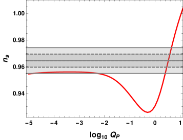
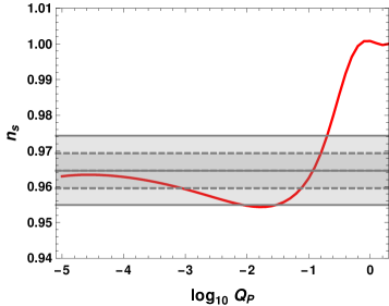
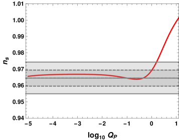
The behaviour of the spectral index nssubscript𝑛𝑠n_{s} as a function of the dissipation parameter QPsubscript𝑄𝑃Q_{P} for all the models we have considered is shown in Fig. 2. To generate these plots in Mathematica, we fixed P(kP)=As=2.2×10⁹subscript𝑃subscript𝑘𝑃subscript𝐴𝑠2.2superscript109P_{\mathcal{R}}(k_{P})=A_{s}=2.2\times 10^{-9} (the value is taken from Ref. [35]) and NP=60subscript𝑁𝑃60N_{P}=60. For a given QPsubscript𝑄𝑃Q_{P} and a fixed NPsubscript𝑁𝑃N_{P}, when we fix the normalisation, Assubscript𝐴𝑠A_{s}, we obtain λ𝜆\lambda and Cϕsubscript𝐶italic-ϕC_{\phi} or CTsubscript𝐶𝑇C_{T}. We then obtain nssubscript𝑛𝑠n_{s}. The colored bands show 68%percent6868\% and 95%percent9595\% C.L. allowed values for nssubscript𝑛𝑠n_{s} for a power law power spectrum from the Planck 2015 TT, TE, EE+low P results [35, 36, 37].
Refer to caption
Refer to caption
Refer to caption
Figure 2: The spectral index, nssubscript𝑛𝑠n_{s} as a function of the dissipation parameter, log10QPsubscript10subscript𝑄𝑃\log_{10}Q_{P} are plotted here (keeping P(kP)=As=2.2×10⁹subscript𝑃subscript𝑘𝑃subscript𝐴𝑠2.2superscript109P_{\mathcal{R}}(k_{P})=A_{s}=2.2\times 10^{-9} and NP=60subscript𝑁𝑃60N_{P}=60) for V(ϕ)=λϕ4𝑉italic-ϕ𝜆superscriptitalic-ϕ4V(\phi)=\lambda\phi^{4} with linear dissipation (Fig. 2) and V(ϕ)=λϕ6MPl2𝑉italic-ϕ𝜆superscriptitalic-ϕ6superscriptsubscript𝑀𝑃𝑙2V(\phi)=\lambda\frac{\phi^{6}}{M_{Pl}^{2}} with linear and cubic dissipation (Fig. 2 and 2 respectively). The band shows the allowed nssubscript𝑛𝑠n_{s} values from Planck 2015 results for a power law power spectrum with 68%percent\% and 95%percent\% C.L.. Each point on the plots corresponds to the values of λ𝜆\lambda and Cϕsubscript𝐶italic-ϕC_{\phi} or CTsubscript𝐶𝑇C_{T} consistent with the power spectrum normalisation and values of QPsubscript𝑄𝑃Q_{P} and NPsubscript𝑁𝑃N_{P}.

For V(ϕ)=λϕ4𝑉italic-ϕ𝜆superscriptitalic-ϕ4V(\phi)=\lambda\phi^{4} and λϕ6MPl2𝜆superscriptitalic-ϕ6superscriptsubscript𝑀𝑃𝑙2\lambda\frac{\phi^{6}}{M_{Pl}^{2}} with the linear dissipation coefficient Υ=CTTΥsubscript𝐶𝑇𝑇\Upsilon=C_{T}T, we have considered both weak and strong dissipative regimes, as shown in Fig. 2 and 2. We see from Fig. 2 that in the weak dissipative regime, not all the values of QPsubscript𝑄𝑃Q_{P} are consistent with observations. Hence for our CosmoMC analysis we run over that particular range of QPsubscript𝑄𝑃Q_{P} only for which nssubscript𝑛𝑠n_{s} is within the allowed range. We also find from Fig. 2 for V(ϕ)=λϕ6MPl2𝑉italic-ϕ𝜆superscriptitalic-ϕ6superscriptsubscript𝑀𝑃𝑙2V(\phi)=\lambda\frac{\phi^{6}}{M_{Pl}^{2}} with the cubic dissipation coefficient Υ=CϕT3ϕ2Υsubscript𝐶italic-ϕsuperscript𝑇3superscriptitalic-ϕ2\Upsilon=C_{\phi}\frac{T^{3}}{\phi^{2}}, that none of the values of QPsubscript𝑄𝑃Q_{P} in the strong dissipative regime are consistent with the allowed range of values. Hence, we consider only the weak dissipative regime for running CosmoMC for this model.

8 Preliminary analysis of the parameters with Mathematica

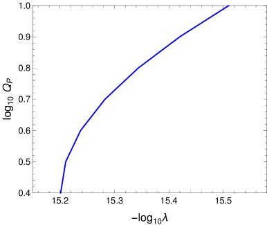
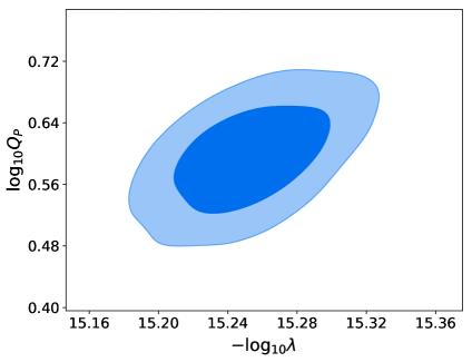
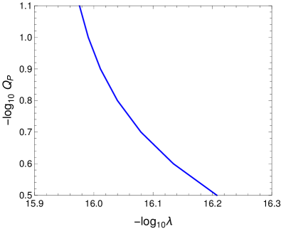
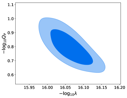
In our models, the primordial power spectrum is written in terms of only two model parameters, λ𝜆\lambda and QPsubscript𝑄𝑃Q_{P}. For our primary analysis in Mathematica, we use the normalisation condition As=2.2×10⁹subscript𝐴𝑠2.2superscript109A_{s}=2.2\times 10^{-9} and obtain the values for λ𝜆\lambda for different QPsubscript𝑄𝑃Q_{P}. However in CosmoMC, we run λ𝜆\lambda and QPsubscript𝑄𝑃Q_{P} independently over an estimated range without the normalisation constraint. We generate the λQP𝜆subscript𝑄𝑃\lambda-Q_{P} plots for the weak and strong dissipative regimes of all the models as shown in the Left plots of Figs. 3, 4, and 6. We expect a similar behaviour to be observed in the CosmoMC analysis. We find that the λQP𝜆subscript𝑄𝑃\lambda-Q_{P} behaviour for the weak dissipative regime is different from the strong dissipative regime by comparing the slopes of the logλlogQP𝜆subscript𝑄𝑃\log\lambda-\log Q_{P} plots. We also estimate the λQP𝜆subscript𝑄𝑃\lambda-Q_{P} relation in Section 9.

9 CosmoMC results

We have carried out a Markov Chain Monte Carlo (MCMC) analysis of our models for the weak and strong dissipation regime using a numerical code CosmoMC (Cosmological Monte Carlo). We run the CosmoMC chains run over a six dimensional parameter space with flat priors on the baryon density Ωbh2subscriptΩ𝑏superscript2\Omega_{b}h^{2}, cold dark matter density Ωch2subscriptΩ𝑐superscript2\Omega_{c}h^{2}, the observed angular size of the sound horizon at recombination θ𝜃\theta, and the reionization optical depth τ𝜏\tau. Along with these, we choose log10λsubscript10𝜆-\log_{10}\lambda and log10QPsubscript10subscript𝑄𝑃-\log_{10}Q_{P} as independent model variables for the weak dissipative regime and log10λsubscript10𝜆-\log_{10}\lambda and log10QPsubscript10subscript𝑄𝑃\log_{10}Q_{P} as independent model variables for the strong dissipative regime in performing our analysis. We take NP=60subscript𝑁𝑃60N_{P}=60 for our entire analysis.

We use the September 2017 version of CAMB and the November 2016 version of CosmoMC and set the flags, compute_tensor=T, CMB_lensing=F, and use_nonlinear_lensing=F. We use as the pivot scale kP=0.05Mpc1subscript𝑘𝑃0.05superscriptMpc1k_{P}=0.05\,\text{Mpc}^{-1}, and perform the CosmoMC analysis with the Planck 2015 TT, TE, EE + low P dataset.

We give below the priors for the parameters of our models and the mean values, along with 68% confidence limits, obtained in the weak and the strong dissipative regimes. For the mean values of our model parameters, λ𝜆\lambda and QPsubscript𝑄𝑃Q_{P}, we also estimate the nssubscript𝑛𝑠n_{s} and r𝑟r. The allowed values of nssubscript𝑛𝑠n_{s} and r𝑟r from the Planck 2015 results (TT, TE, EE+ lowP) [35, 36, 37] are

ns=0.9645±0.0049(68%C.L.)and0.96450.0096+0.0098(95%C.L.)n_{s}=0.9645\pm 0.0049\,(68\%\rm\,C.L.)\qquad and\qquad 0.9645^{+0.0098}_{-0.0096}\,(95\%\rm\,C.L.)
r0.002<0.10(95%C.L.).r_{0.002}<0.10\,(95\%\,\rm{C.L.}). (9.1)

As mentioned in Ref. [35], Planck is sensitive to the tensor modes in the low-l temperature power spectrum and hence the value of the tensor-to-scalar ratio is given at the scale of 0.0020.0020.002 Mpc-1. However, it can be related to the tensor-to-scalar ratio at the scale of 0.050.050.05 Mpc-1 with the relation given in footnote 3 of Ref. [35], and is not very different.

9.1 Model I: V(ϕ)=λϕ4𝑉italic-ϕ𝜆superscriptitalic-ϕ4V(\phi)=\lambda\phi^{4} and Υ=CTTΥsubscript𝐶𝑇𝑇\Upsilon=C_{T}T

We write the priors for the parameters of our model and the mean values along with 68% confidence limits in the weak and the strong dissipative regimes in Tables 1 and 2.

Parameter Priors 68% limits
Ωbh2subscriptΩ𝑏superscript2\Omega_{b}h^{2} [0.005,0.1] 0.02168±0.00014plus-or-minus0.021680.000140.02168\pm 0.00014
Ωch2subscriptΩ𝑐superscript2\Omega_{c}h^{2} [0.001,0.99] 0.1217±0.0010plus-or-minus0.12170.00100.1217\pm 0.0010
100θ100𝜃100\theta [0.50,10.0] 1.040270.00033+0.00029subscriptsuperscript1.040270.000290.000331.04027^{+0.00029}_{-0.00033}
τ𝜏\tau [0.01,0.8] 0.0480.031+0.016subscriptsuperscript0.0480.0160.0310.048^{+0.016}_{-0.031}
log10λsubscript10𝜆-\log_{10}\lambda [13.7,15.5] 14.390.24+0.34subscriptsuperscript14.390.340.2414.39^{+0.34}_{-0.24}
log10QPsubscript10subscript𝑄𝑃-\log_{10}Q_{P} [0.0,5.4] 3.641.1+0.76subscriptsuperscript3.640.761.13.64^{+0.76}_{-1.1}

Mean value of λ𝜆\lambda = 4.07×10154.07superscript10154.07\times 10^{-15}

Mean value of QPsubscript𝑄𝑃Q_{P} = 2.29×1042.29superscript1042.29\times 10^{-4}

For these values, we obtain

ns=0.967subscript𝑛𝑠0.967n_{s}=0.967

r=0.0330𝑟0.0330r=0.0330

Table 1: The priors and the marginalised values along with 68% limits for the parameters of the model V(ϕ)=λϕ4𝑉italic-ϕ𝜆superscriptitalic-ϕ4V(\phi)=\lambda\phi^{4} with Υ=CTTΥsubscript𝐶𝑇𝑇\Upsilon=C_{T}T in the weak dissipative regime are shown here. The mean values of the model parameters and the corresponding values of nssubscript𝑛𝑠n_{s} and r𝑟r are also given.
Parameter Priors 68% limits
Ωbh2subscriptΩ𝑏superscript2\Omega_{b}h^{2} [0.005,0.1] 0.02174±0.00013plus-or-minus0.021740.000130.02174\pm 0.00013
Ωch2subscriptΩ𝑐superscript2\Omega_{c}h^{2} [0.001,0.99] 0.1200±0.0011plus-or-minus0.12000.00110.1200\pm 0.0011
100θ100𝜃100\theta [0.50,10.0] 1.04044±0.00029plus-or-minus1.040440.000291.04044\pm 0.00029
τ𝜏\tau [0.01,0.8] 0.061±0.024plus-or-minus0.0610.0240.061\pm 0.024
log10λsubscript10𝜆-\log_{10}\lambda [15.0,15.6] 15.1660.056+0.036subscriptsuperscript15.1660.0360.05615.166^{+0.036}_{-0.056}
log10QPsubscript10subscript𝑄𝑃\log_{10}Q_{P} [0.0,0.6] <0.156absent0.156<0.156

Mean value of λ𝜆\lambda = 6.82×10166.82superscript10166.82\times 10^{-16}

Upper limit of QPsubscript𝑄𝑃Q_{P} =1.43absent1.43=1.43

For the upper limit, we obtain

ns=0.973subscript𝑛𝑠0.973n_{s}=0.973

r=0.000214𝑟0.000214r=0.000214

Table 2: The priors and the marginalised values along with 68% limits for the parameters of the model V(ϕ)=λϕ4𝑉italic-ϕ𝜆superscriptitalic-ϕ4V(\phi)=\lambda\phi^{4} with Υ=CTTΥsubscript𝐶𝑇𝑇\Upsilon=C_{T}T in the strong dissipative regime are shown here. The mean values of the model parameters and the corresponding values of nssubscript𝑛𝑠n_{s} and r𝑟r are also given.

We can see that the mean values of QPsubscript𝑄𝑃Q_{P} obtained from CosmoMC for the weak and strong dissipative regimes lie in the allowed range of values of QPsubscript𝑄𝑃Q_{P} in the nssubscript𝑛𝑠n_{s} plot in Fig. 2. The values of nssubscript𝑛𝑠n_{s} and r𝑟r obtained from the mean values of λ𝜆\lambda and QPsubscript𝑄𝑃Q_{P} are within the Planck 95%percent\% C.L. in Eq. (9.1).

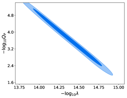
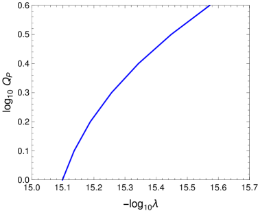
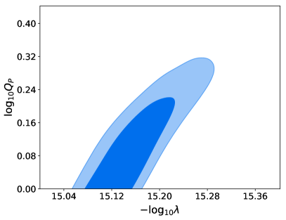
In Fig. 3, we show the joint probability distribution for the QPsubscript𝑄𝑃Q_{P} and λ𝜆\lambda, in the weak and strong dissipative regimes. The Left plots are obtained in Mathematica keeping the normalisation of the primordial power spectrum fixed at a value As=2.2×10⁹subscript𝐴𝑠2.2superscript109A_{s}=2.2\times 10^{-9} and the Right plots are the contour plots with 1σ1𝜎1\sigma and 2σ2𝜎2\sigma regions obtained via CosmoMC.

Refer to caption
Refer to caption
Refer to caption
Refer to caption
Figure 3: Joint probability distribution of log10QPsubscript10subscript𝑄𝑃-\log_{10}Q_{P} and log10λsubscript10𝜆-\log_{10}\lambda for the case V(ϕ)=λϕ4𝑉italic-ϕ𝜆superscriptitalic-ϕ4V(\phi)=\lambda\phi^{4}, with Υ=CTTΥsubscript𝐶𝑇𝑇\Upsilon=C_{T}T in the weak (Top) and between log10QPsubscript10subscript𝑄𝑃\log_{10}Q_{P} and log10λsubscript10𝜆-\log_{10}\lambda in the strong (Bottom) dissipative regime. Left: From Mathematica with the normalisation condition As=2.2×10⁹subscript𝐴𝑠2.2superscript109A_{s}=2.2\times 10^{-9} and Right: from CosmoMC with λ𝜆\lambda and QPsubscript𝑄𝑃Q_{P} as parameters. NP=60subscript𝑁𝑃60N_{P}=60 for all plots.

In the weak dissipative regime, λQP0.3proportional-to𝜆superscriptsubscript𝑄𝑃0.3\lambda\propto Q_{P}^{-0.3} in both the Mathematica and CosmoMC generated plots and for the strong dissipative regime, λQP0.6proportional-to𝜆superscriptsubscript𝑄𝑃0.6\lambda\propto Q_{P}^{-0.6}. One sees that the behaviour of λQP𝜆subscript𝑄𝑃\lambda-Q_{P} differs in the two regimes.

9.2 Model II: V(ϕ)=λϕ6MPl2𝑉italic-ϕ𝜆superscriptitalic-ϕ6superscriptsubscript𝑀𝑃𝑙2V(\phi)=\lambda\frac{\phi^{6}}{M_{Pl}^{2}} and Υ=CTTΥsubscript𝐶𝑇𝑇\Upsilon=C_{T}T

The priors for the model parameters and the mean values along with 68% limits in the weak and the strong dissipative regimes are listed in Tables 3 and 4.

Parameter Priors 68% limits
Ωbh2subscriptΩ𝑏superscript2\Omega_{b}h^{2} [0.005,0.1] 0.02157±0.00013plus-or-minus0.021570.000130.02157\pm 0.00013
Ωch2subscriptΩ𝑐superscript2\Omega_{c}h^{2} [0.001,0.99] 0.12484±0.00099plus-or-minus0.124840.000990.12484\pm 0.00099
100θ100𝜃100\theta [0.50,10.0] 1.03989±0.00029plus-or-minus1.039890.000291.03989\pm 0.00029
τ𝜏\tau [0.01,0.8] 0.056±0.020plus-or-minus0.0560.0200.056\pm 0.020
log10λsubscript10𝜆-\log_{10}\lambda [15.4,16.6] 16.070.19+0.27subscriptsuperscript16.070.270.1916.07^{+0.27}_{-0.19}
log10QPsubscript10subscript𝑄𝑃-\log_{10}Q_{P} [1.8,5.4] 3.540.82+0.68subscriptsuperscript3.540.680.823.54^{+0.68}_{-0.82}

Mean value of λ𝜆\lambda = 8.51×10178.51superscript10178.51\times 10^{-17}

Mean value of QPsubscript𝑄𝑃Q_{P} = 2.88×1042.88superscript1042.88\times 10^{-4}

For these values, we obtain

ns=0.956subscript𝑛𝑠0.956n_{s}=0.956

r=0.0451𝑟0.0451r=0.0451

Table 3: The priors and the marginalised values along with 68% limits for the parameters of the model V(ϕ)=λϕ6MPl2𝑉italic-ϕ𝜆superscriptitalic-ϕ6superscriptsubscript𝑀𝑃𝑙2V(\phi)=\lambda\frac{\phi^{6}}{M_{Pl}^{2}} with Υ=CTTΥsubscript𝐶𝑇𝑇\Upsilon=C_{T}T in the weak dissipative regime are shown here. The mean values of the model parameters and the corresponding values of nssubscript𝑛𝑠n_{s} and r𝑟r are also given.
Parameter Priors 68% limits
Ωbh2subscriptΩ𝑏superscript2\Omega_{b}h^{2} [0.005,0.1] 0.02170±0.00014plus-or-minus0.021700.000140.02170\pm 0.00014
Ωch2subscriptΩ𝑐superscript2\Omega_{c}h^{2} [0.001,0.99] 0.1206±0.0015plus-or-minus0.12060.00150.1206\pm 0.0015
100θ100𝜃100\theta [0.50,10.0] 1.04037±0.00030plus-or-minus1.040370.000301.04037\pm 0.00030
τ𝜏\tau [0.01,0.8] 0.066±0.022plus-or-minus0.0660.0220.066\pm 0.022
log10λsubscript10𝜆-\log_{10}\lambda [14.8,15.9] 15.253±0.029plus-or-minus15.2530.02915.253\pm 0.029
log10QPsubscript10subscript𝑄𝑃\log_{10}Q_{P} [0,1.5] 0.596±0.048plus-or-minus0.5960.0480.596\pm 0.048

Mean value of λ=5.59×10¹⁶𝜆5.59superscript1016\lambda=5.59\times 10^{-16}

Mean value of QPsubscript𝑄𝑃Q_{P} = 3.943.943.94

For these values, we obtain

ns=0.970subscript𝑛𝑠0.970n_{s}=0.970

r=0.0000426𝑟0.0000426r=0.0000426

Table 4: The priors and the marginalised values along with 68% limits for the parameters of the model V(ϕ)=λϕ6MPl2𝑉italic-ϕ𝜆superscriptitalic-ϕ6superscriptsubscript𝑀𝑃𝑙2V(\phi)=\lambda\frac{\phi^{6}}{M_{Pl}^{2}} with Υ=CTTΥsubscript𝐶𝑇𝑇\Upsilon=C_{T}T in the strong dissipative regime are shown here. The mean values of the model parameters and the corresponding values of nssubscript𝑛𝑠n_{s} and r𝑟r are also given.

The mean values of our QPsubscript𝑄𝑃Q_{P} obtained from CosmoMC for the weak and strong dissipative regimes lie in the allowed range of values of QPsubscript𝑄𝑃Q_{P} in the nssubscript𝑛𝑠n_{s} plot in Fig. 2. The values of nssubscript𝑛𝑠n_{s} and r𝑟r obtained from the mean values of λ𝜆\lambda and QPsubscript𝑄𝑃Q_{P} are within the Planck 95%percent\% C.L. as given in Eq. (9.1).

Refer to caption
Refer to caption
Refer to caption
Refer to caption
Figure 4: Joint probability distribution of log10λsubscript10𝜆-\log_{10}\lambda and log10QPsubscript10subscript𝑄𝑃\log_{10}Q_{P} for the case V(ϕ)=λϕ6MPl2𝑉italic-ϕ𝜆superscriptitalic-ϕ6superscriptsubscript𝑀𝑃𝑙2V(\phi)=\lambda\frac{\phi^{6}}{M_{Pl}^{2}}, with Υ=CTTΥsubscript𝐶𝑇𝑇\Upsilon=C_{T}T in the weak (Top) and strong (Bottom) dissipative regime. Left: From Mathematica with the normalisation condition As=2.2×10⁹subscript𝐴𝑠2.2superscript109A_{s}=2.2\times 10^{-9} and Right: from CosmoMC with λ𝜆\lambda and QPsubscript𝑄𝑃Q_{P} as parameters. NP=60subscript𝑁𝑃60N_{P}=60 for all plots.

In Fig. 4, we show the joint probability distribution for the QPsubscript𝑄𝑃Q_{P} and λ𝜆\lambda, in the weak and strong dissipative regimes. Here again, the Left plots are obtained in Mathematica and the Right plots are the contour plots with 1σ1𝜎1\sigma and 2σ2𝜎2\sigma regions obtained via CosmoMC.

In the weak dissipative regime, λQP0.3proportional-to𝜆superscriptsubscript𝑄𝑃0.3\lambda\propto Q_{P}^{-0.3} in both the Mathematica and CosmoMC generated plots and for the strong dissipative regime, λQP0.4proportional-to𝜆superscriptsubscript𝑄𝑃0.4\lambda\propto Q_{P}^{-0.4}. Here also, we can see that the behaviour of λQP𝜆subscript𝑄𝑃\lambda-Q_{P} differs in the two regimes.

9.3 Model III: V(ϕ)=λϕ6MPl2𝑉italic-ϕ𝜆superscriptitalic-ϕ6superscriptsubscript𝑀𝑃𝑙2V(\phi)=\lambda\frac{\phi^{6}}{M_{Pl}^{2}} and Υ=CϕT3ϕ2Υsubscript𝐶italic-ϕsuperscript𝑇3superscriptitalic-ϕ2\Upsilon=C_{\phi}\frac{T^{3}}{\phi^{2}}

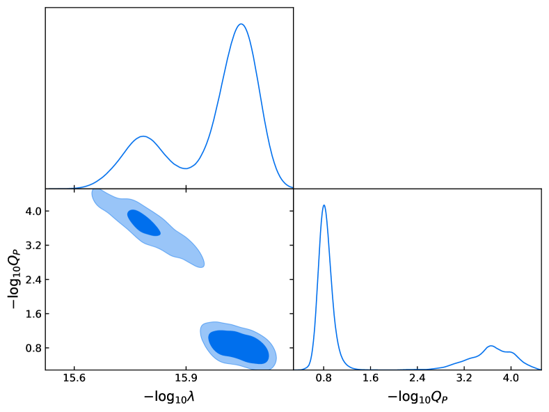
As previously mentioned, in this case, we consider only the weak dissipative regime as the nssubscript𝑛𝑠n_{s} values in the strong dissipation regime overshoot the Planck 2015 allowed region. We obtain two convergence regions in our analysis with CosmoMC. This is shown in Fig. 5. However the region with logQPsubscript𝑄𝑃-\log Q_{P} close to 0 has a higher probability, as shown by the height of the probability distribution peak. Therefore we redo our analysis by restricting the priors such that we only obtain the mean value of QPsubscript𝑄𝑃Q_{P} in the more probable region. We write the priors for the parameters and the mean values along with 68% limits in Table 5.
Refer to caption
Figure 5: Joint probability distribution of log10λsubscript10𝜆-\log_{10}\lambda and log10QPsubscript10subscript𝑄𝑃-\log_{10}Q_{P} for the case V(ϕ)=λϕ6MPl2𝑉italic-ϕ𝜆superscriptitalic-ϕ6superscriptsubscript𝑀𝑃𝑙2V(\phi)=\lambda\frac{\phi^{6}}{M_{Pl}^{2}}, with Υ=CϕT3ϕ2Υsubscript𝐶italic-ϕsuperscript𝑇3superscriptitalic-ϕ2\Upsilon=C_{\phi}\frac{T^{3}}{\phi^{2}} in the weak dissipative regime. The figure shows that there are two convergence regions, however the probability for log10QPsubscript10subscript𝑄𝑃-\log_{10}Q_{P} near 0 is higher as can be seen from the height of the peak.
Parameter Priors 68% limits
Ωbh2subscriptΩ𝑏superscript2\Omega_{b}h^{2} [0.005,0.1] 0.02170±0.00013plus-or-minus0.021700.000130.02170\pm 0.00013
Ωch2subscriptΩ𝑐superscript2\Omega_{c}h^{2} [0.001,0.99] 0.1207±0.0014plus-or-minus0.12070.00140.1207\pm 0.0014
100θ100𝜃100\theta [0.50,10.0] 1.04036±0.00030plus-or-minus1.040360.000301.04036\pm 0.00030
τ𝜏\tau [0.1,0.8] 0.061±0.023plus-or-minus0.0610.0230.061\pm 0.023
log10λsubscript10𝜆-\log_{10}\lambda [15.8,17.0] 16.064±0.38plus-or-minus16.0640.3816.064\pm 0.38
log10QPsubscript10subscript𝑄𝑃-\log_{10}Q_{P} [0,1.5] 0.7990.10+0.068subscriptsuperscript0.7990.0680.100.799^{+0.068}_{-0.10}

Mean value of λ𝜆\lambda =8.63×10178.63superscript10178.63\times 10^{-17}

Mean value of QPsubscript𝑄𝑃Q_{P} =0.15880.15880.1588

For these values, we obtain

ns=0.969subscript𝑛𝑠0.969n_{s}=0.969

r=0.00480𝑟0.00480r=0.00480

Table 5: The priors and the marginalised values along with 68% limits for the parameters of the model V(ϕ)=λϕ6MPl2𝑉italic-ϕ𝜆superscriptitalic-ϕ6superscriptsubscript𝑀𝑃𝑙2V(\phi)=\lambda\frac{\phi^{6}}{M_{Pl}^{2}} with Υ=CϕT3ϕ2Υsubscript𝐶italic-ϕsuperscript𝑇3superscriptitalic-ϕ2\Upsilon=C_{\phi}\frac{T^{3}}{\phi^{2}} in the weak dissipative regime are shown here. The mean values of the model parameters and the corresponding values of nssubscript𝑛𝑠n_{s} and r𝑟r are also given.
Refer to caption
Refer to caption
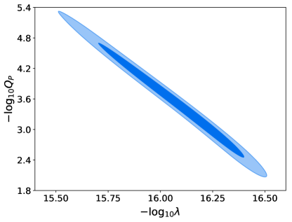
Figure 6: Joint probability distribution of log10λsubscript10𝜆-\log_{10}\lambda and log10QPsubscript10subscript𝑄𝑃-\log_{10}Q_{P} for the case V(ϕ)=λϕ6MPl2𝑉italic-ϕ𝜆superscriptitalic-ϕ6superscriptsubscript𝑀𝑃𝑙2V(\phi)=\lambda\frac{\phi^{6}}{M_{Pl}^{2}}, with Υ=CϕT3ϕ2Υsubscript𝐶italic-ϕsuperscript𝑇3superscriptitalic-ϕ2\Upsilon=C_{\phi}\frac{T^{3}}{\phi^{2}} in the weak dissipative regime. Left: From Mathematica with the normalisation condition (As=2.2×10⁹subscript𝐴𝑠2.2superscript109A_{s}=2.2\times 10^{-9}) and Right: from CosmoMC with λ𝜆\lambda and QPsubscript𝑄𝑃Q_{P} as parameters. NP=60subscript𝑁𝑃60N_{P}=60 for all plots.

The mean values of our QPsubscript𝑄𝑃Q_{P} obtained from CosmoMC for the weak dissipative regime lie in the allowed range of values of QPsubscript𝑄𝑃Q_{P} in the nssubscript𝑛𝑠n_{s} plot in Fig. 2. The value of nssubscript𝑛𝑠n_{s} obtained from the mean values of λ𝜆\lambda and QPsubscript𝑄𝑃Q_{P} is within the Planck 68%percent\% C.L. in Eq. (9.1) while the value of r𝑟r is consistent with the Planck bounds.

In Fig. 6, we show the joint probability distribution for the QPsubscript𝑄𝑃Q_{P} and λ𝜆\lambda, in the weak dissipative regime. Here again, the Left plot is obtained in Mathematica and the Right plot is the contour plot with 1σ1𝜎1\sigma and 2σ2𝜎2\sigma regions obtained via CosmoMC.

The relation between λQP𝜆subscript𝑄𝑃\lambda-Q_{P} goes as λQP0.4proportional-to𝜆superscriptsubscript𝑄𝑃0.4\lambda\propto Q_{P}^{-0.4} in the weak dissipative regime, which is similar in both the Mathematica and CosmoMC analyses.

10 Conclusion

In standard cold inflation, the inflaton’s couplings with other fields are ineffective during the inflationary phase and as a result the Universe is supercooled during inflation. Warm inflation provides an alternate picture of inflation where radiation production takes place concurrent to the inflationary phase and the Universe has a temperature during inflation. With the current measurements of temperature anisotropies in the Cosmic Microwave Background radiation, various monomial potentials of standard cold inflation are ruled out from the nsrsubscript𝑛𝑠𝑟n_{s}-r parameter space. However, certain monomial potentials are still viable models in the context of warm inflation.

As an extension to our previous study on estimating the parameters of warm inflationary λϕ4𝜆superscriptitalic-ϕ4\lambda\phi^{4} potential with a cubic dissipation coefficient, here we have discussed the λϕ4𝜆superscriptitalic-ϕ4\lambda\phi^{4} potential model of warm inflation with a linear dissipation coefficient and the λϕ6𝜆superscriptitalic-ϕ6\lambda\phi^{6} potential model of warm inflation with linear and cubic dissipation coefficients. We have shown the dynamics of the inflaton and radiation during warm inflation. We parameterize the primordial power spectrum for our models and study its dependence on the model parameters, namely, λ𝜆\lambda signifying the inflaton self coupling, and QPsubscript𝑄𝑃Q_{P}, representing the dissipation parameter arising because of the inflaton’s couplings to the other fields. After a preliminary analysis using Mathematica, we perform a Markov Chain Monte Carlo (MCMC) analysis over these model parameters and four standard parameters using the CosmoMC numerical code. This provides us the mean values of all the parameters with 68%percent6868\% confidence limits for all the models we consider. For the mean values of parameters, we also estimate the values for the spectral tilt, nssubscript𝑛𝑠n_{s} and the tensor-to-scalar ratio r𝑟r and find them to be consistent with the Planck allowed ranges for all the models we consider. We also obtain the joint probability contours with 1σ1𝜎1\sigma and 2σ2𝜎2\sigma regions for λ𝜆\lambda and QPsubscript𝑄𝑃Q_{P} with the GetDist package. For all the models, we approximate a linear fit to the joint probability curve of logλ𝜆\log\lambda and logQPsubscript𝑄𝑃\log Q_{P} and find a relation between them. An estimation of the parameters of warm inflation models and the relations between them is important from the perspective of model building.

For the weak dissipative region, our values of r𝑟r for the mean values of the model parameters is within the sensitivity of order 103superscript10310^{-3} of the next generation of ground-based and satellite-based CMB polarisation experiments [38, 39, 40]. However, for the strong dissipative region, the corresponding values of r𝑟r are lower than the sensitivity of these future experiments. It has been argued that lensing of intensity fluctuations in the 21-cm signal from atomic hydrogen in the dark ages can in principle provide a probe of inflationary gravitational waves down to a sensitivity of 109superscript10910^{-9} for r𝑟r [41]. However such measurements would be challenging and require a futuristic experiment. Experiments have also been proposed to measure the redshifted 21-cm hydrogen line and use interferometry to obtain a sensitivity of 103superscript10310^{-3} on the Earth, and a sensitivity of 106superscript10610^{-6} with an array of detectors covering a large area of the Moon’s surface [42]. Thus while the warm inflation models studied here for the weak dissipative regime can be further investigated via CMB polarisation experiments in the near future, one will have to wait much longer to test these models in the strong dissipative regime.

Acknowledgements
The results presented in the paper are based on the computations using Vikram-100, the 100TFLOP HPC Cluster at Physical Research Laboratory, Ahmedabad, India. We would like to thank Prakrut Chaubal and Jayanti Prasad for their help in CosmoMC related issues. We would also like to thank Gaurav Goswami, Namit Mahajan and Arvind Kumar Mishra for valuable discussions and suggestions.

\appendixpage

Appendix A Dissipation parameter at the end of inflation, and the integral function

For V(ϕ)=λϕ4𝑉italic-ϕ𝜆superscriptitalic-ϕ4V(\phi)=\lambda\phi^{4} with Υ=CTTΥsubscript𝐶𝑇𝑇\Upsilon=C_{T}T

The positive real solution to Eq. (7.9) is given by

Qe(λ,CT)=231/3Y(9Y+327Y24Y3)1/3+(9Y+327Y24Y3)1/321/332/3subscript𝑄𝑒𝜆subscript𝐶𝑇superscript2313𝑌superscript9𝑌327superscript𝑌24superscript𝑌313superscript9𝑌327superscript𝑌24superscript𝑌313superscript213superscript323Q_{e}(\lambda,C_{T})=\frac{\frac{2}{3}^{1/3}Y}{(9Y+\sqrt{3}\sqrt{27Y^{2}-4Y^{3}})^{1/3}}+\frac{(9Y+\sqrt{3}\sqrt{27Y^{2}-4Y^{3}})^{1/3}}{{2}^{1/3}{3}^{2/3}} (A.1)

where Y=11234Cϕ49Aλ.𝑌1superscript1234superscriptsubscript𝐶italic-ϕ49𝐴𝜆Y=\frac{1}{12^{3}}\frac{4C_{\phi}^{4}}{9A\lambda}. In this way, Qesubscript𝑄𝑒Q_{e} is expressed in terms of λ𝜆\lambda and CTsubscript𝐶𝑇C_{T}.
The integral function in Eq. (7.13) is given as

F(Q)=1Z3(1+Q)13(2+3F12(1,1;5/3;1/Q))2Q𝐹𝑄1𝑍3superscript1𝑄1323subscriptsubscript𝐹1211531𝑄2𝑄F(Q)=\frac{1}{Z}\frac{-3(1+Q)^{\frac{1}{3}}(2+3\,\,{{}_{2}F_{1}}(1,1;5/3;-1/Q))}{2Q} (A.2)

where Z=124(4CT49Aλ)1/3𝑍124superscript4superscriptsubscript𝐶𝑇49𝐴𝜆13Z=\frac{1}{24}\left(\frac{4C_{T}^{4}}{9A\lambda}\right)^{1/3} and F12(a,b;c;z)subscriptsubscript𝐹12𝑎𝑏𝑐𝑧{{}_{2}F_{1}}(a,b;c;z) is the hypergeometric function.

For V(ϕ)=λϕ6MPl2𝑉italic-ϕ𝜆superscriptitalic-ϕ6superscriptsubscript𝑀𝑃𝑙2V(\phi)=\lambda\frac{\phi^{6}}{M_{Pl}^{2}} with Υ=CTTΥsubscript𝐶𝑇𝑇\Upsilon=C_{T}T

The positive real solution to Eq. (7.11) is given by

Qe(λ,CT)subscript𝑄𝑒𝜆subscript𝐶𝑇\displaystyle Q_{e}(\lambda,C_{T}) =Y3+21/3(6Y+Y2)3(27Y+18Y2+2Y3+33(27Y2+4Y3)1/3\displaystyle=\frac{Y}{3}+\frac{2^{1/3}(6Y+Y^{2})}{3(27Y+18Y^{2}+2Y^{3}+3\sqrt{3}\sqrt{(27Y^{2}+4Y^{3}})^{1/3}}
+(27Y+18Y2+2Y3+33(27Y2+4Y3)1/321/3 3\displaystyle+\frac{(27Y+18Y^{2}+2Y^{3}+3\sqrt{3}\sqrt{(27Y^{2}+4Y^{3}})^{1/3}}{2^{1/3}\,3} (A.3)

where Y=1304CT48πAλ.𝑌1superscript304superscriptsubscript𝐶𝑇48𝜋𝐴𝜆Y=\frac{1}{30^{4}}\frac{C_{T}^{4}8\pi}{A\lambda}. In this way, Qesubscript𝑄𝑒Q_{e} is expressed in terms of λ𝜆\lambda and CTsubscript𝐶𝑇C_{T}.

The integral function in Eq. (7.13) is given as

F(Q)=1Z4((1+Q)124QF12(1/4,1/2;5/4;Q))Q34𝐹𝑄1𝑍4superscript1𝑄124𝑄subscriptsubscript𝐹12141254𝑄superscript𝑄34F(Q)=\frac{1}{Z}\frac{4((1+Q)^{\frac{1}{2}}-4\,\,Q\,\,{{}_{2}F_{1}}(1/4,1/2;5/4;-Q))}{Q^{\frac{3}{4}}} (A.4)

where Z=π6(CT4Aλ(8π)3)1/4.𝑍𝜋6superscriptsuperscriptsubscript𝐶𝑇4𝐴𝜆superscript8𝜋314Z=\frac{\pi}{6}\left(\frac{C_{T}^{4}}{A\lambda(8\pi)^{3}}\right)^{1/4}.

For V(ϕ)=λϕ6MPl2𝑉italic-ϕ𝜆superscriptitalic-ϕ6superscriptsubscript𝑀𝑃𝑙2V(\phi)=\lambda\frac{\phi^{6}}{M_{Pl}^{2}} with Υ=CϕT3ϕ2Υsubscript𝐶italic-ϕsuperscript𝑇3superscriptitalic-ϕ2\Upsilon=C_{\phi}\frac{T^{3}}{\phi^{2}}

The positive real solution to Eq. (7.12) is given by

Qe(λ,Cϕ)=13(2+21/3(2+27Y+334Y+27Y2)1/3+(2+27Y+334Y+27Y2)1/321/3)subscript𝑄𝑒𝜆subscript𝐶italic-ϕ132superscript213superscript227𝑌334𝑌27superscript𝑌213superscript227𝑌334𝑌27superscript𝑌213superscript213Q_{e}(\lambda,C_{\phi})=\frac{1}{3}\left(-2+\frac{2^{1/3}}{(2+27Y+3\sqrt{3}\sqrt{4Y+27Y^{2}})^{1/3}}+\frac{(2+27Y+3\sqrt{3}\sqrt{4Y+27Y^{2}})^{1/3}}{2^{1/3}}\right) (A.5)

where Y=1104λCϕ48πA3.𝑌1superscript104𝜆superscriptsubscript𝐶italic-ϕ48𝜋superscript𝐴3Y=\frac{1}{10^{4}}\frac{\lambda C_{\phi}^{4}}{8\pi A^{3}}. In this way, Qesubscript𝑄𝑒Q_{e} is expressed in terms of λ𝜆\lambda and Cϕsubscript𝐶italic-ϕC_{\phi}.

The integral function in Eq. (7.13) is given as

F(Q)=1Z4+8Q8/3Q(1+Q)F12(1,5/4;7/4;Q)Q1/4(1+Q)1/2𝐹𝑄1𝑍48𝑄83𝑄1𝑄subscriptsubscript𝐹1215474𝑄superscript𝑄14superscript1𝑄12F(Q)=\frac{1}{Z}\frac{-4+8Q-8/3Q(1+Q)\,\,{{}_{2}F_{1}}(1,5/4;7/4;-Q)}{Q^{1/4}(1+Q)^{1/2}} (A.6)

where Z=116(λCϕ48πA3)1/4.𝑍116superscript𝜆superscriptsubscript𝐶italic-ϕ48𝜋superscript𝐴314Z=\frac{1}{16}\left(\frac{\lambda C_{\phi}^{4}}{8\pi A^{3}}\right)^{1/4}.

Appendix B Expression of the spectral index, nssubscript𝑛𝑠n_{s}

For V(ϕ)=λϕ4𝑉italic-ϕ𝜆superscriptitalic-ϕ4V(\phi)=\lambda\phi^{4} with Υ=CTTΥsubscript𝐶𝑇𝑇\Upsilon=C_{T}T

nssubscript𝑛𝑠\displaystyle n_{s} =19ϵH(1+QP)(1ϵH)(3+5QP)+X(2HPTPexp(HPTP)nP2+TPHP23πQP3+4πQP6+6πQP3+4πQP)absent19subscriptitalic-ϵ𝐻1subscript𝑄𝑃1subscriptitalic-ϵ𝐻35subscript𝑄𝑃𝑋2subscript𝐻𝑃subscript𝑇𝑃subscript𝐻𝑃subscript𝑇𝑃superscriptsubscript𝑛𝑃2subscript𝑇𝑃subscript𝐻𝑃23𝜋subscript𝑄𝑃34𝜋subscript𝑄𝑃66𝜋subscript𝑄𝑃34𝜋subscript𝑄𝑃\displaystyle=1-\frac{9\epsilon_{H}(1+Q_{P})}{(1-\epsilon_{H})(3+5\,Q_{P})}+X\left(\frac{2H_{P}}{T_{P}}\exp\left(\frac{H_{P}}{T_{P}}\right)n_{P}^{2}+\frac{T_{P}}{H_{P}}\frac{2\sqrt{3}\pi Q_{P}}{\sqrt{3+4\pi Q_{P}}}\,\frac{6+6\pi Q_{P}}{3+4\pi Q_{P}}\right)
+3ϵH(1ϵH)QP(1+QP)3+5QP0.042827QP1.315+0.45694QP0.3641+0.0185QP2.315+0.335QP1.3643subscriptitalic-ϵ𝐻1subscriptitalic-ϵ𝐻subscript𝑄𝑃1subscript𝑄𝑃35subscript𝑄𝑃0.042827superscriptsubscript𝑄𝑃1.3150.45694superscriptsubscript𝑄𝑃0.36410.0185superscriptsubscript𝑄𝑃2.3150.335superscriptsubscript𝑄𝑃1.364\displaystyle+\frac{3\epsilon_{H}}{(1-\epsilon_{H})}\frac{Q_{P}(1+Q_{P})}{3+5\,Q_{P}}\,\frac{0.042827\,Q_{P}^{1.315}+0.45694\,Q_{P}^{0.364}}{1+0.0185\,Q_{P}^{2.315}+0.335\,Q_{P}^{1.364}} (B.1)

where X=1[1+2nP+(TPHP)23πQP3+4πQP]3ϵH(1+QP)(1ϵH)(3+5QP)𝑋1delimited-[]12subscript𝑛𝑃subscript𝑇𝑃subscript𝐻𝑃23𝜋subscript𝑄𝑃34𝜋subscript𝑄𝑃3subscriptitalic-ϵ𝐻1subscript𝑄𝑃1subscriptitalic-ϵ𝐻35subscript𝑄𝑃X=\frac{1}{\left[1+2n_{P}+\left(\frac{T_{P}}{H_{P}}\right)\frac{2\sqrt{3}\pi Q_{P}}{\sqrt{3+4\pi Q_{P}}}\right]}\,\,\frac{3\epsilon_{H}(1+Q_{P})}{(1-\epsilon_{H})(3+5\,Q_{P})} and ϵHsubscriptitalic-ϵ𝐻\epsilon_{H} is evaluated at k=kP.𝑘subscript𝑘𝑃k=k_{P}.

For V(ϕ)=λϕ6MPl2𝑉italic-ϕ𝜆superscriptitalic-ϕ6superscriptsubscript𝑀𝑃𝑙2V(\phi)=\lambda\frac{\phi^{6}}{M_{Pl}^{2}} with Υ=CTTΥsubscript𝐶𝑇𝑇\Upsilon=C_{T}T

nssubscript𝑛𝑠\displaystyle n_{s} =18ϵH(1+QP)(1ϵH)(3+5QP)+X(2HPTPexp(HPTP)nP2+TPHP23πQP3+4πQP6+6πQP3+4πQP)absent18subscriptitalic-ϵ𝐻1subscript𝑄𝑃1subscriptitalic-ϵ𝐻35subscript𝑄𝑃𝑋2subscript𝐻𝑃subscript𝑇𝑃subscript𝐻𝑃subscript𝑇𝑃superscriptsubscript𝑛𝑃2subscript𝑇𝑃subscript𝐻𝑃23𝜋subscript𝑄𝑃34𝜋subscript𝑄𝑃66𝜋subscript𝑄𝑃34𝜋subscript𝑄𝑃\displaystyle=1-\frac{8\epsilon_{H}(1+Q_{P})}{(1-\epsilon_{H})(3+5\,Q_{P})}+X\left(\frac{2H_{P}}{T_{P}}\exp\left(\frac{H_{P}}{T_{P}}\right)n_{P}^{2}+\frac{T_{P}}{H_{P}}\frac{2\sqrt{3}\pi Q_{P}}{\sqrt{3+4\pi Q_{P}}}\,\frac{6+6\pi Q_{P}}{3+4\pi Q_{P}}\right)
+8ϵH3(1ϵH)QP(1+QP)3+5QP0.042827QP1.315+0.45694QP0.3641+0.0185QP2.315+0.335QP1.3648subscriptitalic-ϵ𝐻31subscriptitalic-ϵ𝐻subscript𝑄𝑃1subscript𝑄𝑃35subscript𝑄𝑃0.042827superscriptsubscript𝑄𝑃1.3150.45694superscriptsubscript𝑄𝑃0.36410.0185superscriptsubscript𝑄𝑃2.3150.335superscriptsubscript𝑄𝑃1.364\displaystyle+\frac{8\epsilon_{H}}{3(1-\epsilon_{H})}\frac{Q_{P}(1+Q_{P})}{3+5\,Q_{P}}\,\frac{0.042827\,Q_{P}^{1.315}+0.45694\,Q_{P}^{0.364}}{1+0.0185\,Q_{P}^{2.315}+0.335\,Q_{P}^{1.364}} (B.2)

where X=1[1+2nP+(TPHP)23πQP3+4πQP]8ϵH(1+QP)3(1ϵH)(3+5QP)𝑋1delimited-[]12subscript𝑛𝑃subscript𝑇𝑃subscript𝐻𝑃23𝜋subscript𝑄𝑃34𝜋subscript𝑄𝑃8subscriptitalic-ϵ𝐻1subscript𝑄𝑃31subscriptitalic-ϵ𝐻35subscript𝑄𝑃X=\frac{1}{\left[1+2n_{P}+\left(\frac{T_{P}}{H_{P}}\right)\frac{2\sqrt{3}\pi Q_{P}}{\sqrt{3+4\pi Q_{P}}}\right]}\,\,\frac{8\epsilon_{H}(1+Q_{P})}{3(1-\epsilon_{H})(3+5\,Q_{P})} and ϵHsubscriptitalic-ϵ𝐻\epsilon_{H} is evaluated at k=kP.𝑘subscript𝑘𝑃k=k_{P}.

For V(ϕ)=λϕ6MPl2𝑉italic-ϕ𝜆superscriptitalic-ϕ6superscriptsubscript𝑀𝑃𝑙2V(\phi)=\lambda\frac{\phi^{6}}{M_{Pl}^{2}} with Υ=CϕT3ϕ2Υsubscript𝐶italic-ϕsuperscript𝑇3superscriptitalic-ϕ2\Upsilon=C_{\phi}\frac{T^{3}}{\phi^{2}}

nssubscript𝑛𝑠\displaystyle n_{s} =18ϵH(1+5QP)3(1ϵH)(1+7QP)+X(2HPTPexp(HPTP)nP2+TPHP23πQP3+4πQP(1+2(1+QP)(3+2πQP)(1+3QP)(3+4πQP)))absent18subscriptitalic-ϵ𝐻15subscript𝑄𝑃31subscriptitalic-ϵ𝐻17subscript𝑄𝑃𝑋2subscript𝐻𝑃subscript𝑇𝑃subscript𝐻𝑃subscript𝑇𝑃superscriptsubscript𝑛𝑃2subscript𝑇𝑃subscript𝐻𝑃23𝜋subscript𝑄𝑃34𝜋subscript𝑄𝑃121subscript𝑄𝑃32𝜋subscript𝑄𝑃13subscript𝑄𝑃34𝜋subscript𝑄𝑃\displaystyle=1-\frac{8\epsilon_{H}(1+5\,Q_{P})}{3(1-\epsilon_{H})(1+7\,Q_{P})}+X\left(\frac{2H_{P}}{T_{P}}\exp\left(\frac{H_{P}}{T_{P}}\right)n_{P}^{2}+\frac{T_{P}}{H_{P}}\frac{2\sqrt{3}\pi Q_{P}}{\sqrt{3+4\pi Q_{P}}}\left(1+\frac{2(1+Q_{P})(3+2\pi Q_{P})}{(1+3\,Q_{P})(3+4\pi Q_{P})}\right)\right)
+8ϵH3(1ϵH)QP(1+QP)1+7QP9.693026QP0.946+0.54991QP3.3301+4.981QP1.946+0.127QP4.3308subscriptitalic-ϵ𝐻31subscriptitalic-ϵ𝐻subscript𝑄𝑃1subscript𝑄𝑃17subscript𝑄𝑃9.693026superscriptsubscript𝑄𝑃0.9460.54991superscriptsubscript𝑄𝑃3.33014.981superscriptsubscript𝑄𝑃1.9460.127superscriptsubscript𝑄𝑃4.330\displaystyle+\frac{8\epsilon_{H}}{3(1-\epsilon_{H})}\frac{Q_{P}(1+Q_{P})}{1+7\,Q_{P}}\,\,\frac{9.693026\,Q_{P}^{0.946}+0.54991\,Q_{P}^{3.330}}{1+4.981\,Q_{P}^{1.946}+0.127\,Q_{P}^{4.330}} (B.3)

where X=1[1+2nP+(TPHP)23πQP3+4πQP]4ϵH(1+3QP)3(1ϵH)(1+7QP)𝑋1delimited-[]12subscript𝑛𝑃subscript𝑇𝑃subscript𝐻𝑃23𝜋subscript𝑄𝑃34𝜋subscript𝑄𝑃4subscriptitalic-ϵ𝐻13subscript𝑄𝑃31subscriptitalic-ϵ𝐻17subscript𝑄𝑃X=\frac{1}{\left[1+2n_{P}+\left(\frac{T_{P}}{H_{P}}\right)\frac{2\sqrt{3}\pi Q_{P}}{\sqrt{3+4\pi Q_{P}}}\right]}\,\,\frac{4\epsilon_{H}(1+3Q_{P})}{3(1-\epsilon_{H})(1+7Q_{P})} and ϵHsubscriptitalic-ϵ𝐻\epsilon_{H} is evaluated at k=kP.𝑘subscript𝑘𝑃k=k_{P}.

References

  • [1] A. A. Starobinsky, “A New Type of Isotropic Cosmological Models Without Singularity,” Phys. Lett. B 91, 99 (1980).
  • [2] D. Kazanas, “Dynamics of the Universe and Spontaneous Symmetry Breaking,” Astrophys. J.  241, L59 (1980).
  • [3] K. Sato, “First Order Phase Transition of a Vacuum and Expansion of the Universe,” Mon. Not. Roy. Astron. Soc.  195, 467 (1981).
  • [4] A. H. Guth, “The Inflationary Universe: A Possible Solution to the Horizon and Flatness Problems,” Phys. Rev. D 23, 347 (1981).
  • [5] A. D. Linde, “A New Inflationary Universe Scenario: A Possible Solution of the Horizon, Flatness, Homogeneity, Isotropy and Primordial Monopole Problems,” Phys. Lett.  108B, 389 (1982).
  • [6] A. Albrecht and P. J. Steinhardt, “Cosmology for Grand Unified Theories with Radiatively Induced Symmetry Breaking,” Phys. Rev. Lett.  48, 1220 (1982).
  • [7] A. D. Linde, “Chaotic Inflation,” Phys. Lett.  129B, 177 (1983).
  • [8] D. Baumann, TASI-2009 lectures, “Inflation,” arXiv:0907.5424 [hep-th].
  • [9] A. Riotto, “Inflation and the theory of cosmological perturbations,” ICTP Lect. Notes Ser.  14, 317 (2003). [hep-ph/0210162].
  • [10] L. Kofman, A. D. Linde and A. A. Starobinsky, “Reheating after inflation,” Phys. Rev. Lett.  73, 3195 (1994).
  • [11] A. Berera and L. Z. Fang, “Thermally induced density perturbations in the inflation era,” Phys. Rev. Lett.  74, 1912 (1995)
  • [12] A. Berera, “Warm inflation,” Phys. Rev. Lett.  75, 3218 (1995).
  • [13] A. Berera, M. Gleiser and R. O. Ramos, “A First principles warm inflation model that solves the cosmological horizon / flatness problems,” Phys. Rev. Lett.  83, 264 (1999)
  • [14] A. Berera, I. G. Moss and R. O. Ramos, “Warm Inflation and its Microphysical Basis,” Rept. Prog. Phys.  72, 026901 (2009).
  • [15] R. Rangarajan, “Current Status of Warm Inflation,” arXiv:1801.02648 [astro-ph.CO].
  • [16] M. Bastero-Gil and A. Berera, “Warm inflation model building,” Int. J. Mod. Phys. A 24, 2207 (2009).
  • [17] G. Panotopoulos and N. Videla, “Warm λ4ϕ4𝜆4superscriptitalic-ϕ4\frac{\lambda}{4}\phi^{4} inflationary universe model in light of Planck 2015 results,” Eur. Phys. J. C 75, no. 11, 525 (2015).
  • [18] L. Visinelli, “Observational Constraints on Monomial Warm Inflation,” JCAP 1607, no. 07, 054 (2016).
  • [19] M. Benetti and R. O. Ramos, “Warm inflation dissipative effects: predictions and constraints from the Planck data,” Phys. Rev. D 95, 023517 (2017).
  • [20] R. Arya, A. Dasgupta, G. Goswami, J. Prasad and R. Rangarajan, “Revisiting CMB constraints on warm inflation,” JCAP 1802, no. 02, 043 (2018).
  • [21] M. Bastero-Gil, A. Berera and N. Kronberg, “Exploring the Parameter Space of Warm-Inflation Models,” JCAP 1512, no. 12, 046 (2015).
  • [22] C. P. Burgess, M. Majumdar, D. Nolte, F. Quevedo, G. Rajesh and R. J. Zhang, “The Inflationary brane anti-brane universe,” JHEP 0107, 047 (2001).
  • [23] H. Mishra, S. Mohanty and A. Nautiyal, “Warm natural inflation,” Phys. Lett. B 710, 245 (2012).
  • [24] M. Bastero-Gil, A. Berera, R. O. Ramos and J. G. Rosa, “Warm Little Inflaton,” Phys. Rev. Lett.  117, 151301 (2016).
  • [25] A. Lewis and S. Bridle, “Cosmological parameters from CMB and other data: A Monte Carlo approach,” Phys. Rev. D 66, 103511 (2002).
  • [26] L. M. H. Hall, I. G. Moss and A. Berera, “Scalar perturbation spectra from warm inflation,” Phys. Rev. D 69, 083525 (2004).
  • [27] I. G. Moss and C. Xiong, “On the consistency of warm inflation,” JCAP 0811, 023 (2008).
  • [28] R. O. Ramos and L. A. da Silva, “Power spectrum for inflation models with quantum and thermal noises,” JCAP 1303, 032 (2013).
  • [29] I. G. Moss and C. Xiong, “Dissipation coefficients for supersymmetric inflatonary models,” hep-ph/0603266.
  • [30] M. Bastero-Gil, A. Berera and R. O. Ramos, “Dissipation coefficients from scalar and fermion quantum field interactions,” JCAP 1109, 033 (2011).
  • [31] M. Bastero-Gil, A. Berera, R. O. Ramos and J. G. Rosa, “General dissipation coefficient in low-temperature warm inflation,” JCAP 1301, 016 (2013).
  • [32] S. Bartrum, M. Bastero-Gil, A. Berera, R. Cerezo, R. O. Ramos and J. G. Rosa, “The importance of being warm (during inflation),” Phys. Lett. B 732, 116 (2014).
  • [33] C. Graham and I. G. Moss, “Density fluctuations from warm inflation,” JCAP 0907, 013 (2009).
  • [34] M. Bastero-Gil, S. Bhattacharya, K. Dutta and M. R. Gangopadhyay, “Constraining Warm Inflation with CMB data,” JCAP 1802, no. 02, 054 (2018).
  • [35] P. A. R. Ade et al. [Planck Collaboration], “Planck 2015 results. XIII. Cosmological parameters,” Astron. Astrophys.  594, A13 (2016) (Table 4).
  • [36] P. A. R. Ade et al. [Planck Collaboration], “Planck 2015 results. XX. Constraints on inflation,” Astron. Astrophys.  594, A20 (2016).
  • [37] https://wiki.cosmos.esa.int/planck-legacy-archive/images/1/1a/Baseline__\_params__\_table__\_2015__\_limit95.pdf
    (Table 2.6).
  • [38] K. N. Abazajian et al. [CMB-S4 Collaboration], “CMB-S4 Science Book, First Edition,” arXiv:1610.02743 [astro-ph.CO].
  • [39] H. Ishino et al., “LiteBIRD: lite satellite for the study of B-mode polarization and inflation from cosmic microwave background radiation detection,” Proc. SPIE Int. Soc. Opt. Eng.  9904, 99040X (2016).
  • [40] P. Creminelli, D. L. López Nacir, M. Simonović, G. Trevisan and M. Zaldarriaga, “Detecting Primordial B𝐵B-Modes after Planck,” JCAP 1511, no. 11, 031 (2015).
  • [41] L. Book, M. Kamionkowski and F. Schmidt, “Lensing of 21-cm Fluctuations by Primordial Gravitational Waves,” Phys. Rev. Lett.  108, 211301 (2012).
  • [42] R. Ansari et al. [Cosmic Visions 21 cm Collaboration], “Inflation and Early Dark Energy with a Stage II Hydrogen Intensity Mapping experiment,” arXiv:1810.09572 [astro-ph.CO].