Range-separated tensor representation of the discretized multidimensional Dirac delta and
elliptic operator inverse

Abstract

In this paper, we introduce the operator dependent range-separated tensor approximation of the discretized Dirac delta in $\mathbb{R}^{d}$. It is constructed by application of the discrete elliptic operator to the range-separated decomposition of the associated Green kernel discretized on the Cartesian grid in $\mathbb{R}^{d}$. The presented operator dependent local-global splitting of the Dirac delta can be applied for solving the potential equations in non-homogeneous medium when the density in the right-hand side is given by the large sum of pointwise singular charges. We show how the idea of the operator dependent RS splitting of the Dirac delta can be extended to the closely related problem on the range separated tensor representation of the elliptic resolvent. The numerical tests confirm the expected localization properties of the obtained operator dependent approximation of the Dirac delta represented on a tensor grid. As an example of application, we consider the regularization scheme for solving the Poisson-Boltzmann equation for modeling the electrostatics in bio-molecules.

Key words: Coulomb potential, Green function, Dirac delta, long-range many-particle interactions, low-rank tensor decomposition, range-separated tensor formats, summation of electrostatic potentials.

AMS Subject Classification: 65F30, 65F50, 65N35, 65F10

1 Introduction

The grid-based approximation of the multidimensional Dirac delta function arises in modeling of the long-range potentials in multiparticle systems in variety of applications. For example, in potential equations describing electrostatics of large biomolecules, in molecular dynamics simulations of large solvated biological systems, in docking or folding of proteins, pattern recognition and many other problems [14, 23, 24]. Furthermore, in PDE driven models via elliptic operators in $\mathbb{R}^{d}$ with constant coefficients the Dirac delta naturally arises as the singular point density specifying the definition of the corresponding fundamental solution (the Green kernel). In what follows, we rely on the new concept of operator dependent Dirac delta in elliptic problems, where this function can be associated, for example, with the harmonic or bi-harmonic operator, in representation of elastic and hydrodynamics potentials in 3D elasticity problems, or in the fundamental solution of advection-diffusion operator with constant coefficients in $\mathbb{R}^{3}$.

In the approaches based on the potential energy ansatz, the potential elliptic equations usually include the “multiparticle” Dirac delta function, which is used for modeling the density of charges, smeared over the compact part of the computational domain in the course of the solution process. Due to strong singularity in the Dirac delta such computational schemes are error prone owing to strict limitations on the 3D grid size, when using the traditional grid based numerical methods. These restrictions lead to quite heavy computation task using rather coarse available grids, considerably reducing the capabilities of numerical simulations when using the Dirac delta function in modeling of many-particle systems. The attempts based on analytic pre-computation of the free space component in the collective potential on a 3D grid may cause some other numerical troubles.

In this paper, we introduce the new method for the operator dependent approximation of the Dirac delta in $\mathbb{R}^{d}$ by using the range-separated (RS) tensor representation [2, 3] of the Green kernel for certain elliptic operator discretized over tensor product Cartesian grids with the large grid size. To fix the idea, we consider the radial function $p(x)=p(\|x\|)$ specifying the Green’s kernel (fundamental solution) for a second order elliptic operator $\cal L$ with constant coefficients, such that the equation

$${\cal L}p(\|x\|)=\delta(\|x\|),\quad x=(x_{1},\ldots,x_{d})\in\mathbb{R}^{d}$$ (1.1)

holds, where $\delta(x)$ is the operator dependent Dirac delta function in $\mathbb{R}^{d}$ (tempered distribution). Assume that both the operator ${\cal L}$ and the Green kernel $p(\|x\|)$ are represented in a low-rank tensor formats on the $d$-fold $n\times\cdots\times n$ Cartesian grid in $\mathbb{R}^{d}$. Now for given RS type tensor decomposition of the discretized Green kernel

$$p(\|x\|)=p_{s}(\|x\|)+p_{l}(\|x\|),$$ (1.2)

we introduce the RS tensor splitting of the discretized Dirac delta associated with the operator ${\cal L}$,

$$\delta(\|x\|)={\cal L}p_{s}(\|x\|)+{\cal L}p_{l}(\|x\|):=\delta_{s}(\|x\|)+\delta_{l}(\|x\|),$$ (1.3)

where both terms in the right-hand side can be rewritten in the low rank tensor form. Here $\delta_{s}(\|x\|)$ and $\delta_{l}(\|x\|)$ represent the grid-based decomposition of the Dirac delta into the short- and long-range components, where the latter is smooth enough.

This introduces the smoothing operation for the discretized Dirac delta, such that the target function $\delta(\|x\|)$ is recovered from the smoothed version by the highly localized short-range correction. The total error in the tensor decomposition is controlled by the $\varepsilon$-truncation rank parameters and by the one-dimensional size $n$ of the representation grid in $\mathbb{R}^{d}$. Using tensor approach, the grid-based multidimensional Dirac delta is presented with a controllable accuracy level, which is practically not possible in the traditional numerical methods. Notice that the main idea of the approach was reported by the author in a brief form in the monograph [22], §5.8.1.

The idea of the operator dependent RS splitting of the Dirac delta can be extended to the closely related problem on the range separated tensor representation of the elliptic resolvent. In Section 4, we discuss the concept of the RS splitting for the elliptic operator inverse and present some examples demonstrating the application of this new approach to variety of elliptic operators with constant coefficients.

Our techniques can be extended to the RS splitting of the multiparticle Dirac delta. In this case, the calculation of the long-range part in the collective Dirac delta can be viewed as the smoothing procedure for highly singular functions in the right-hand site of the potential equation. Specifically, for a given generating radial function $p(x)=p(\|x\|)$, $x\in\mathbb{R}^{3}$ the calculation and meshing up of a weighted sum of interaction potentials in the large $N$-particle system, with the particle locations $x_{\nu}\in\mathbb{R}^{3}$, and charges $q_{\nu}\in\mathbb{R}$, $\nu=1,...,N$,

$$P_{0}(x)={\sum}_{\nu=1}^{N}{q_{\nu}}\,p({\|x-x_{\nu}\|}),\quad x_{\nu},x\in\Omega=[-b,b]^{3},$$ (1.4)

leads to computationally intensive numerical task. Indeed, the commonly used generating radial functions $p(\|x\|)$ exhibit a slow polynomial decay $O(\|x\|^{-\alpha})$, $\alpha>0$ as $\|x\|\to\infty$ so that each individual term in (1.4) contributes essentially to the total potential at each point in the computational box $\Omega$. This anticipates the $O(N)$ complexity for the straightforward summation at every fixed target $x\in\mathbb{R}^{3}$, resulting in $O(N^{2})$ complexity for the energy calculation and $O(n^{3}N)$ cost for the meshing up the $n\times n\times n$ grid. Moreover, in many cases, the radial function $p(\|x\|)$ has a singularity or a cusp at the origin, $x=0$, making its accurate grid representation problematic.

Our method allows calculation of the long-range part of the “collective “ Dirac delta in the RS tensor format, which is implemented via one-dimensional operations and with the linear complexity in the number of particles $N$ requiring only $O(n\log^{q}N)$ storage size.

The commonly used example of the harmonic Green kernel is given by

$$p(\|x\|)=\frac{\Gamma(d/2-1)}{4\pi^{d/2}\|x\|^{d-2}},\quad\mbox{for}\quad{\cal L}=-\Delta,\quad x\in\mathbb{R}^{d},$$

where $\Delta$ denotes the Laplace operator in $\mathbb{R}^{d}$

$$\Delta=\sum\limits_{\ell=1}^{d}\frac{\partial^{2}}{\partial x^{2}_{\ell}}.$$

For $d=3$ the function $p(\|x\|)$ coincides with the classical Newton kernel

$$p(\|x\|)=\frac{1}{4\pi\|x\|}\quad\mbox{(the Coulomb potential).}$$ (1.5)

In this case the solution $u(x)$ of the Poisson equation (see also (4.2))

$$-\Delta u=f$$

is called the harmonic potential of the density $f$.

The Yukawa and Helmholtz kernels in $\mathbb{R}^{3}$ are given by $\frac{e^{-\kappa\|x\|}}{4\pi\|x\|}$ corresponding to the choice ${\cal L}=-\Delta\pm\kappa^{2}$, $\kappa\in\mathbb{C}$. The large class of the so-called Matèrn radial functions (see [25] and references therein) includes the Slater function $e^{-\kappa\|x\|}$, $\kappa\in(0,\infty)$ and the dipole-dipole interaction kernel $1/\|x\|^{3}$, for $x\in\mathbb{R}^{3}$.

Tensor-based approach provides efficient computation of the collective long-range potential of a many-particle system in homogeneous media, see for example assembled tensor method [16, 17] for finite lattices, or the RS tensor format [2, 3] for the many-particle systems of general type. The collective electrostatic potential on a 3D lattice is computed by one-dimensional translations and summations, while the RS tensor method provides computations with linear complexity in the number of particles, $O(N)$ and linear-logarithmic cost the univariate grid size, $O(n\log^{q}n)$, but not as $O(n^{3})$. However, development of these methods for biomolecular modeling is a forthcoming problem, and the present paper makes a step forward to the efficient solution of this problem.

The modern techniques for computation of the collective electrostatic potential in heterogeneous media in biomolecular modeling (as well as in docking and classification problems) are based on numerical solution of the elliptic equations in $\mathbb{R}^{3}$ with non-constant permeability, where the right-hand side is represented by a large sum of weighted delta functions (see example of the computational domain in Figure 1.1). In this model the solute (molecular) region $\Omega_{m}$ consists of the union of small balls of radius $\sigma>0$ around the atomic centers (see §3.3 for the detailed discussion).

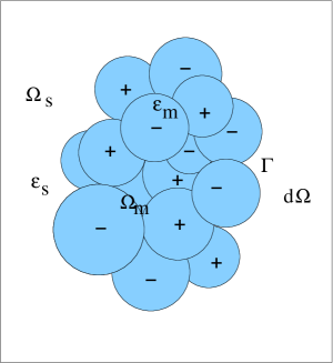
Figure 1.1: Solute and solvent regions $\Omega_{m}$ and $\Omega_{s}$ in the computational domain $\Omega$ for the Poisson-Boltzmann model.

In electrostatic calculations the radial function is given by the Newton kernel (1.5), such that the free space electrostatic potential $P_{0}(x)$ in (1.4) satisfies the potential equation

$$-\Delta P_{0}(x)={\sum}_{\nu=1}^{N}{q_{\nu}}\,\delta({\|x-x_{\nu}\|})\quad\mbox{in}\quad\mathbb{R}^{3},$$

with highly singular multiparticle Dirac delta in the right-hand side. The latter equation may be incorporated into the more complicated elliptic equation with jumping coefficients across the irregular interface and with possible nonlinearity (see Fig. 1.1 and the related example of the Poisson-Boltzmann equation in §3.3 also considered in [4]). The RS decomposition of the multiparticle Dirac delta introduced in this paper provides the efficient way for regularization of the solution scheme for the arising elliptic boundary value problem.

The rest of the paper is organized as follows. In Section 2, we recall the main ingredients for the grid-based tensor representation of the multivariate interaction potentials. The brief introduction to the RS tensor formats is also provided. Section 3 describes the main ingredients in the grid-based RS tensor splitting of the Dirac delta. We present several examples of elliptic PDEs where the RS tensor can be applied to both the fundamental solutions and to the corresponding operator dependent Dirac delta. In Section 4 we discuss the closely related concept of the RS splitting for the elliptic operator inverse and provide several examples demonstrating the application of this new approach. In Conclusions, we summarize the main features of the proposed numerical scheme and overview some possible application.

2 Tensor representation of multiparticle interaction potentials

Recent tensor-structured numerical methods appeared as a bridging of the the approximation theory for the multidimensional functions and operators [11, 10, 20] with the rank-structured tensor formats from multilinear algebra [29]. One of the important results in these developments was the efficient method for summation of the electrostatic potentials in molecular systems. The starting point was the grid based computation of the nuclear potential operator for molecules in the framework of the Hartree-Fock equation [18, 15], where the canonical tensor representation of the Newton kernel was applied and the controllable accuracy is provided due to large 3D Cartesian grids.

The tensor-structured representation of the Coulomb potential became especially advantageous in grid-based assembled summation of the long-range potentials on large lattices. This method was introduced in [16], where it was proven that the tensor rank of a collective electrostatic potential of an arbitrarily large 3D lattice is the same as the canonical rank of a single Newton kernel. For lattices of non-rectangular shapes or in presence of defects the tensor ranks was shown to increase only slightly [17].

2.1 Rank-structured tensor representation of radial functions

First, we recall the grid-based method for the low-rank canonical representation of a spherically symmetric kernel function $p(\|x\|)$, $x\in\mathbb{R}^{d}$ for $d=2,3,\ldots$, by its projection onto the set of piecewise constant basis functions. In the case of Newton and Yukawa Green’s kernels

$$p(\|x\|)=\frac{1}{4\pi\|x\|},\quad\mbox{ and }\quad p(\|x\|)=\frac{e^{-\lambda\|x\|}}{4\pi\|x\|},\quad x\in\mathbb{R}^{3}$$ (2.1)

the numerical scheme for their representation on a fine 3D $n\times n\times n$ Cartesian grid in the form low-rank canonical tensor was described in [20, 5]. The corresponding approximation theory for the class of reference potentials like $p(\|x\|)$ in (2.1) was presented in [11, 20, 22].

In what follows, for the ease of exposition, we confine ourselves to the case $d=3$ though that the sinc-quadrature based separable approximation of the radial functions apply for the arbitrary dimension $d$. In the computational domain $\Omega=[-b,b]^{3}$, let us introduce the uniform $n\times n\times n$ rectangular Cartesian grid $\Omega_{n}$ with mesh size $h=2b/n$ ($n$ even). Let $\{\psi_{\textbf{i}}\}$ be a set of tensor-product piecewise constant basis functions,

$$\psi_{\textbf{i}}(\textbf{x})=\prod_{\ell=1}^{3}\psi_{i_{\ell}}^{(\ell)}(x_{\ell}),$$ (2.2)

for the $3$-tuple index ${\bf i}=(i_{1},i_{2},i_{3})$, $i_{\ell}\in I_{\ell}=\{1,...,n\}$, $\ell=1,\,2,\,3$. The generating kernel $p(\|x\|)$ is discretized by its projection onto the basis set $\{\psi_{\textbf{i}}\}$ in the form of a third order tensor of size $n\times n\times n$, defined entry-wise as

$$\mathbf{P}:=[p_{\bf i}]\in\mathbb{R}^{n\times n\times n},\quad p_{\bf i}=\int_{\mathbb{R}^{3}}\psi_{\bf i}({x})p(\|{x}\|)\,\,\mathrm{d}{x}.$$ (2.3)

The low-rank canonical decomposition of the $3$rd order tensor $\mathbf{P}$ is based on using exponentially convergent $\operatorname*{sinc}$-quadratures for approximating the Laplace-Gauss transform to the analytic function $p(z)$, $z\in\mathbb{C}$, specified by a certain weight $\widehat{p}(t)>0$,

$$p(z)=\int_{\mathbb{R}_{+}}\widehat{p}(t)e^{-t^{2}z^{2}}\,\mathrm{d}t\approx\sum_{k=-M}^{M}p_{k}e^{-t_{k}^{2}z^{2}}\quad\mbox{for}\quad|z|>0,\quad z\in\mathbb{R},$$ (2.4)

with the proper choice of the quadrature points $t_{k}$ and weights $p_{k}$. Under the assumption $0<a\leq|z|<\infty$ this quadrature can be proven to provide an exponential convergence rate in $M$ for a class of analytic functions $p(z)$. The $sinc$-quadrature based approximation to generating function by using the short-term Gaussian sums in (2.4), (2.9) are applicable to the class of analytic functions in certain strip $|z|\leq D$ in the complex plane, such that on the real axis these functions decay polynomially or exponentially. We refer to basic results in [30, 7, 11], where the exponential convergence of the $sinc$-approximation in the number of terms (i.e., the canonical rank) was analyzed. Now, for any fixed $x=(x_{1},x_{2},x_{3})\in\mathbb{R}^{3}$, such that $\|{x}\|>a>0$, we apply the $\operatorname*{sinc}$-quadrature approximation (2.4), (2.9) to obtain the separable expansion

$$p({\|{x}\|})=\int_{\mathbb{R}_{+}}\widehat{p}(t)e^{-t^{2}\|{x}\|^{2}}\,\mathrm{d}t\approx\sum_{k=-M}^{M}p_{k}e^{-t_{k}^{2}\|{x}\|^{2}}=\sum_{k=-M}^{M}p_{k}\prod_{\ell=1}^{3}e^{-t_{k}^{2}x_{\ell}^{2}},$$ (2.5)

providing an exponential convergence rate in $M$,

$$\left|p({\|{x}\|})-\sum_{k=-M}^{M}p_{k}e^{-t_{k}^{2}\|{x}\|^{2}}\right|\leq\frac{C}{a}\,\displaystyle{e}^{-\beta\sqrt{M}},\quad\text{with some}\ C,\beta>0.$$ (2.6)

Combining (2.3) and (2.5), and taking into account the separability of the Gaussian basis functions, we arrive at the low-rank approximation to each entry of the tensor $\mathbf{P}$,

$$p_{\bf i}\approx\sum_{k=-M}^{M}p_{k}\int_{\mathbb{R}^{3}}\psi_{\bf i}({x})e^{-t_{k}^{2}\|{x}\|^{2}}\mathrm{d}{x}=\sum_{k=-M}^{M}p_{k}\prod_{\ell=1}^{3}\int_{\mathbb{R}}\psi^{(\ell)}_{i_{\ell}}(x_{\ell})e^{-t_{k}^{2}x^{2}_{\ell}}\mathrm{d}x_{\ell}.$$

Define the vector (recall that $p_{k}>0$)

$$\textbf{p}^{(\ell)}_{k}=p_{k}^{1/3}\left[b^{(\ell)}_{i_{\ell}}(t_{k})\right]_{i_{\ell}=1}^{n_{\ell}}\in\mathbb{R}^{n_{\ell}}\quad\text{with }\quad b^{(\ell)}_{i_{\ell}}(t_{k})=\int_{\mathbb{R}}\psi^{(\ell)}_{i_{\ell}}(x_{\ell})e^{-t_{k}^{2}x^{2}_{\ell}}\mathrm{d}x_{\ell},$$ (2.7)

then the $3$rd order tensor $\mathbf{P}$ can be approximated by the $R$-term ($R=2M+1$) canonical representation

$$\mathbf{P}\approx\mathbf{P}_{R}=\sum_{k=-M}^{M}p_{k}\bigotimes_{\ell=1}^{3}{\bf b}^{(\ell)}(t_{k})=\sum\limits_{k=-M}^{M}{\bf p}^{(1)}_{k}\otimes{\bf p}^{(2)}_{k}\otimes{\bf p}^{(3)}_{k}\in\mathbb{R}^{n\times n\times n},$$ (2.8)

where ${\bf p}^{(\ell)}_{k}\in\mathbb{R}^{n}$. Given a threshold $\varepsilon>0$, $M$ can be chosen as the minimal number such that in the max-norm

$$\|\mathbf{P}-\mathbf{P}_{R}\|\leq\varepsilon\|\mathbf{P}\|.$$

The skeleton vectors can be re-numerated by $k\mapsto q=k+M+1$, ${\bf p}^{(\ell)}_{k}\mapsto{\bf p}^{(\ell)}_{q}$, ($q=1,...,R$), $\ell=1,2,3$. The canonical tensor ${\bf P}_{R}$ in (2.8) approximates the 3D symmetric kernel function $p({\|x\|})$ ($x\in\Omega$), centered at the origin, such that ${\bf p}^{(1)}_{q}={\bf p}^{(2)}_{q}={\bf p}^{(3)}_{q}$ ($q=1,...,R$).

In the case of Newton kernel we have $p(z)=1/z$, $\widehat{p}(t)=\frac{2}{\sqrt{\pi}}$, and the Laplace-Gauss transform representation reads

$$\frac{1}{z}=\frac{2}{\sqrt{\pi}}\int_{\mathbb{R}_{+}}e^{-z^{2}t^{2}}dt,\quad\mbox{where}\quad z=\|x\|,\quad x\in\mathbb{R}^{3}$$

that can be rewritten the form (by using the substitution $t=\log(1+e^{u})$)

$$\frac{1}{z}=\frac{2}{\sqrt{\pi}}\int_{\mathbb{R}}f_{1}(u,z)du,\quad\mbox{with}\quad f_{1}(u,z)=\frac{e^{-z^{2}\log^{2}(1+e^{u})}}{(1+e^{-u})}.$$

Then the second substitution leads to the integral representation

$$\frac{1}{z}=\frac{2}{\sqrt{\pi}}\int_{\mathbb{R}}F(w,z)dw,\quad F(w,z):=\mbox{cosh}(w)f_{1}(\mbox{sinh}(w),z),$$

such that the set of quadrature points and discretized integrand can be chosen by

$$w_{k}=k\mathfrak{h}_{M},\quad F_{k}=F(w_{k},z)\mathfrak{h}_{M},\quad\mathfrak{h}_{M}=C_{0}/\sqrt{M},\quad C_{0}>0,$$ (2.9)

providing the exponential convergence rate as in (2.6).

One can observe form numerical tests that there are canonical vectors representing the long- and short-range (highly localized) contributions to the total electrostatic potential. This interesting feature was also recognized for the rank-structured tensors representing a lattice sum of electrostatic potentials [16, 17].

2.2 Tensor splitting of the kernel into long- and short-range parts

From the definition of the quadrature (2.8), (2.9), we can easily observe that the full set of approximating Gaussians includes two classes of functions: those with small ”effective support” and the long-range functions. Consequently, functions from different classes may require different tensor-based schemes for their efficient numerical treatment. Hence, the idea of the new approach is the constructive implementation of a range separation scheme that allows the independent efficient treatment of both the long- and short-range parts in each summand in (1.4).

In what follows, without loss of generality, we confine ourselves to the case of the Newton kernel in $\mathbb{R}^{3}$, so that the sum in (2.8) via (2.9) reduces to $k=0,1,\ldots,M$ (due to symmetry argument). From (2.9) we observe that the sequence of quadrature points $\{t_{k}\}$, can be split into two subsequences, ${\cal T}:=\{t_{k}|k=0,1,\ldots,M\}={\cal T}_{l}\cup{\cal T}_{s},$ with

$${\cal T}_{l}:=\{t_{k}\,|k=0,1,\ldots,R_{l}\},\quad\mbox{and}\quad{\cal T}_{s}:=\{t_{k}\,|k=R_{l}+1,\ldots,M\}.$$ (2.10)

Here ${\cal T}_{l}$ includes quadrature points $t_{k}$ condensed “near” zero, hence generating the long-range Gaussians (low-pass filters), and ${\cal T}_{s}$ accumulates the increasing in $M\to\infty$ sequence of “large” sampling points $t_{k}$ with the upper bound $C_{0}^{2}\log^{2}(M)$, corresponding to the short-range Gaussians (high-pass filters). Notice that the quasi-optimal choice of the constant $C_{0}\approx 3$ was determined in [5]. We further denote ${\cal K}_{l}:=\{k\,|k=0,1,\ldots,R_{l}\}$ and ${\cal K}_{s}:=\{k\,|k=R_{l}+1,\ldots,M\}$.

Splitting (2.10) generates the additive decomposition of the canonical tensor $\mathbf{P}_{R}$ onto the short- and long-range parts,

$$\mathbf{P}_{R}=\mathbf{P}_{R_{s}}+\mathbf{P}_{R_{l}},$$

where

$$\mathbf{P}_{R_{s}}=\sum\limits_{t_{k}\in{\cal T}_{s}}{\bf p}^{(1)}_{k}\otimes{\bf p}^{(2)}_{k}\otimes{\bf p}^{(3)}_{k},\quad\mathbf{P}_{R_{l}}=\sum\limits_{t_{k}\in{\cal T}_{l}}{\bf p}^{(1)}_{k}\otimes{\bf p}^{(2)}_{k}\otimes{\bf p}^{(3)}_{k}.$$ (2.11)

The choice of the critical number $R_{l}=\#{\cal T}_{l}-1$ (or equivalently, $R_{s}=\#{\cal T}_{s}=M-R_{l}$), that specifies the splitting ${\cal T}={\cal T}_{l}\cup{\cal T}_{s}$, is determined by the active support of the short-range components such that one can cut off the functions ${\bf p}_{k}(x)$, $t_{k}\in{\cal T}_{s}$, outside of the sphere $B_{\sigma}$ of radius ${\sigma}>0$, subject to a certain threshold $\delta>0$. For fixed $\delta>0$, the choice of $R_{s}$ is uniquely defined by the (small) parameter $\sigma$ and vise versa. Given $\sigma$, the following two basic criteria, corresponding to (A) the max- and (B) $L^{1}$-norm estimates can be applied:

$$(A)\quad{\cal T}_{s}=\{t_{k}:\,a_{k}e^{-t_{k}^{2}\sigma^{2}}\leq\delta\}\;\Leftrightarrow\;R_{l}=\min k:\,a_{k}e^{-t_{k}^{2}\sigma^{2}}\leq\delta,$$ (2.12)

$$(B)\quad{\cal T}_{s}:=\{t_{k}:\,a_{k}\int_{B_{\sigma}}e^{-t_{k}^{2}x^{2}}dx\leq\delta\}\;\Leftrightarrow\;R_{l}=\min k:\,a_{k}\int_{B_{\sigma}}e^{-t_{k}^{2}x^{2}}dx\leq\delta.$$ (2.13)

The quantitative estimates on the value of $R_{l}$ can be easily calculated by using the explicit equation (2.9) for the quadrature parameters. For example, in case $C_{0}=3$ and $a(t)=1$, criteria (A) implies that $R_{l}$ solves the equation

$$\left(\frac{3R_{l}\log M}{M}\right)^{2}\sigma^{2}=\log(\frac{\mathfrak{h}_{M}}{\delta}).$$

Criteria (2.12) and (2.13) can be modified depending on the particular applications. For example, in electronic structure calculations, the parameter $\sigma$ can be associated with the typical inter-atomic distance in the molecular system of interest.

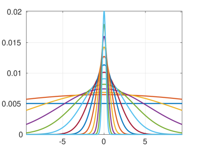
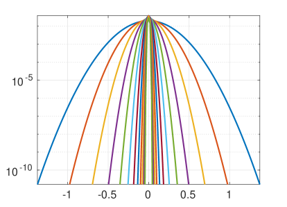
Figure 2.1: Long-range vectors (left) and and short-range (in logarithmic scale) canonical vectors for $n=1024$, $R=24,RL=13$.

Figure 2.1 illustrates the splitting (2.10) for the tensor ${\bf P}_{R}={\bf P}_{R_{l}}+{\bf P}_{R_{s}}$ in (2.11) represented on the $n\times n\times n$ grid with the parameters $R=20,R_{l}=12$ and $R_{s}=8$, respectively (cf. [3]). Following criteria (A) with $\delta\approx 10^{-4}$, the effective support for this splitting is determined by $\sigma=0.9$. The complete Newton kernel depicted in Figure 3.2, left, exhibits the long-range behavior, while the function values of the tensor ${\bf P}_{R_{s}}$ decay exponentially fast apart of the effective support, see Figure 2.1, right.

Inspection of the quadrature point distribution in (2.9) shows that the short- and long-range subsequences are nearly equally balanced distributed, so that one can expect approximately

$$R_{s}\approx R_{l}=M/2.$$ (2.14)

The optimal choice may depend on the particular kernel function and applications.

The advantage of the range separation in the splitting of the canonical tensor

$${\bf P}_{R}\mapsto{\bf P}_{R_{s}}+{\bf P}_{R_{l}}$$

in (2.11) is the opportunity for independent tensor representations of both sub-tensors ${\bf P}_{R_{s}}$ and ${\bf P}_{R_{l}}$ providing the separate treatment of the short- and long-range parts in the total sum of many pointwise interaction potentials as in (1.4).

2.3 Brief introduction to the RS tensor format

The novel range separated (RS) tensor format has been recently introduced in [2, 3]. This format is well suited for modeling of the long-range interaction potential in multi-particle systems. It is based on the partitioning of the reference tensor representation of the newton kernel into long-range and short-range part.

According to the tensor canonical representation of the Newton kernel (2.8) as a sum of Gaussians, one can distinguish their supports into the short- and long-range parts, $\mathbf{P}_{R}=\mathbf{P}_{R_{s}}+\mathbf{P}_{R_{l}},$ given by (2.11). Then the RS splitting (2.11) is applied to the reference canonical tensor ${\bf P}_{R}$ and to its accompanying version $\widetilde{\bf P}_{R}=[\widetilde{p}_{R}(i_{1},i_{2},i_{3})]$, $i_{\ell}\in\widetilde{I}_{\ell}$, $\ell=1,2,3$ living on the double size grid with the same mesh size, such that

$$\widetilde{\bf P}_{R}=\widetilde{\mathbf{P}}_{R_{s}}+\widetilde{\mathbf{P}}_{R_{l}}\in\mathbb{R}^{2n\times 2n\times 2n}.$$

The total electrostatic potential $P_{0}(x)$ in (1.4) is represented by a projected tensor ${\bf P}_{0}\in\mathbb{R}^{n\times n\times n}$ that can be constructed by a direct sum of shift-and-windowing transforms of the reference tensor $\widetilde{\bf P}_{R}$ (see [16] for more details),

$${\bf P}_{0}=\sum_{\nu=1}^{N}{z_{\nu}}\,{\cal W}_{\nu}(\widetilde{\bf P}_{R})=\sum_{\nu=1}^{N}{z_{\nu}}\,{\cal W}_{\nu}(\widetilde{\mathbf{P}}_{R_{s}}+\widetilde{\mathbf{P}}_{R_{l}})=:{\bf P}_{s}+{\bf P}_{l}.$$ (2.15)

The shift-and-windowing transform ${\cal W}_{\nu}$ maps a reference tensor $\widetilde{\bf P}_{R}\in\mathbb{R}^{2n\times 2n\times 2n}$ onto its sub-tensor of smaller size $n\times n\times n$, obtained by first shifting the center of the reference tensor $\widetilde{\bf P}_{R}$ to the grid-point $x_{\nu}$ and then restricting (windowing) the result onto the computational grid $\Omega_{n}$.

The difficulty of the tensor representation (2.15) is that the number of terms in the canonical representation of the full tensor sum ${\bf P}_{0}$ increases almost proportionally to the number $N$ of particles in the system. And it is not tractable for the rank reduction [2].

This problem is solved in [2, 3] by considering the global tensor decomposition of only the ”long-range part” in the tensor ${\bf P}_{0}$, defined by

$${\bf P}_{l}=\sum_{\nu=1}^{N}{z_{\nu}}\,{\cal W}_{\nu}(\widetilde{\mathbf{P}}_{R_{l}})=\sum_{\nu=1}^{N}{z_{\nu}}\,{\cal W}_{\nu}(\sum\limits_{k\in{\cal K}_{l}}\widetilde{\bf p}^{(1)}_{k}\otimes\widetilde{\bf p}^{(2)}_{k}\otimes\widetilde{\bf p}^{(3)}_{k}).$$ (2.16)

And for tensor representation of the sums of short-range parts, a sum of cumulative tensors of small support (and small size) is used, accomplished by the list of the 3D potentials coordinates.

In what follows, we recall the definition of the RS tensor format

Definition 2.1

(RS-canonical tensors [2, 3]). Given the separation parameter $\gamma\in\mathbb{N}$ and a set of points $x_{\nu}\in\mathbb{R}^{d}$, $\nu=1,\ldots,N$, the RS-canonical tensor format specifies the class of $d$-tensors ${\bf A}\in\mathbb{R}^{n_{1}\times\cdots\times n_{d}}$ which can be represented as a sum of a rank-${R}_{L}$ canonical tensor

$${\bf A}_{R_{L}}={\sum}_{k=1}^{R_{L}}\xi_{k}{\bf a}_{k}^{(1)}\otimes\cdots\otimes{\bf a}_{k}^{(d)}\in\mathbb{R}^{n_{1}\times...\times n_{d}}$$

and a cumulated canonical tensor

$$\widehat{\bf A}_{S}={\sum}_{\nu=1}^{N}c_{\nu}{\bf A}_{\nu},$$

generated by replication of the reference tensor ${\bf A}_{0}$ to the points $x_{\nu}$. Then the RS canonical tensor is presented as

$${\bf A}={\bf A}_{R_{L}}+\widehat{\bf A}_{S}={\sum}_{k=1}^{R_{L}}\xi_{k}{\bf a}_{k}^{(1)}\otimes\cdots\otimes{\bf a}_{k}^{(d)}+{\sum}_{\nu=1}^{N}c_{\nu}{\bf A}_{\nu},$$ (2.17)

where $\mbox{rank}({\bf A}_{0})\leq R_{0}$ and $\mbox{diam}(\mbox{supp}{\bf U}_{0})\leq 2\gamma$ in the index size.

The storage size for the RS-canonical tensor ${\bf A}$ in (2.17) is estimated by ([3], Lemma 3.9),

$$\mbox{stor}({\bf A})\leq dRn+(d+1)N+dR_{0}\gamma.$$

Denote by $\overline{\bf u}^{(\ell)}_{i_{\ell}}\in\mathbb{R}^{1\times R}$ the row-vector with index $i_{\ell}$ in the side matrix $U^{(\ell)}\in\mathbb{R}^{n_{\ell}\times R}$ of ${\bf U}$, and by $\xi=(\xi_{1},\ldots,\xi_{d})$ the coefficient vector in (2.17). Then the ${\bf i}$-th entry of the RS-canonical tensor ${\bf A}=[a_{\bf i}]$ can be calculated as a sum of long- and short-range contributions by

$$a_{\bf i}=\left(\odot_{\ell=1}^{d}\overline{\bf u}^{(\ell)}_{i_{\ell}}\right)\xi^{T}+\sum_{\nu\in{\cal L}({\bf i})}c_{\nu}{\bf U}_{\nu}({\bf i}),\quad\mbox{at the expense}\quad O(dR+2d\gamma R_{0}).$$

In application to the calculation of multi-particle interaction potentials discussed above we associate the tensors ${\bf P}_{s}$ and ${\bf P}_{l}$ in (2.15) with short- and long-range components ${\bf A}_{R_{L}}$ and $\widehat{\bf A}_{S}$ in the RS representation of the collective electrostatic potential ${\bf P}_{0}$. The following theorem proofs the almost uniform in $N$ bound on the Tucker (and canonical) rank of the tensor ${\bf A}_{R_{L}}={\bf P}_{l}$, representing the long-range part of ${\bf P}_{0}$.

Theorem 2.2

(Uniform rank bounds for the long-range part, [2, 3]). Let the long-range part ${\bf P}_{l}$ in the total interaction potential, see (2.16), correspond to the choice of splitting parameter in (2.14) with $M=O(\log^{2}\varepsilon)$. Then the total $\varepsilon$-rank ${\bf r}_{0}$ of the Tucker approximation to the canonical tensor sum ${\bf P}_{l}$ is bounded by

$$|{\bf r}_{0}|:=rank_{Tuck}({\bf P}_{l})=C\,b\,\log^{3/2}(|\log(\varepsilon/N)|),$$ (2.18)

where the constant $C$ does not depend on the number of particles $N$.

3 Operator dependent RS tensor decomposition of the $\delta$-function

In this section, we propose the new splitting scheme for the elliptic problem which is based on the range separated representation of the $\delta$-function which enters the highly singular right-hand side in the target elliptic PDE, say, for the Poisson-Boltzmann model (3.5) considered below.

3.1 Overlook on explicit approximations of the Dirac delta

The commonly used approximation of the $\delta$-function can be constructed in the form of Gaussian $C(\lambda)\mbox{e}^{-\lambda^{2}\|x\|^{2}}$ as $\lambda\to\infty$. Let $d=3$, the harmonic potential of the $3$-dimensional Gaussian $f(x)=\mbox{e}^{-\lambda^{2}\|x\|^{2}}$ is represented by using the erf-function

$${\cal L}^{-1}(\mbox{e}^{-\lambda^{2}\|\cdot\|^{2}})(x)=\frac{1}{4\pi}\int_{\mathbb{R}^{3}}\frac{\mbox{e}^{-\lambda^{2}\|y\|^{2}}}{\|x-y\|}dy=\frac{1}{2\|\lambda x\|}\int_{0}^{\|\lambda x\|}\mbox{e}^{-t^{2}}\,dt=\frac{\sqrt{\pi}}{4\lambda\|x\|}\mbox{erf}(\|\lambda x\|).$$

This provides the corresponding approximant to the Green kernel, which, however does not lead to the range-separated representation in question.

Notice that the alternative non-smooth approximation to the Dirac delta by the step-type bumps

$$\delta_{h}(x):=h^{-d},\quad\mbox{if}\quad|x_{\ell}|\leq h,\;\ell=1,\ldots,d;\quad 0\;\;\mbox{otherwise},$$

does not allow to catch the short- and long-range parts of the Green kernels of interest.

For the range-separated tensor representation, we apply the “clever” constructed weighted sum of Gaussian-type functions $\Sigma_{M}=\sum_{k=1}^{M}p_{k}e^{\lambda_{k}\|x\|^{2}}$ (see §2.1 on the sinc quadrature based approach) to approximate the Green kernel and, respectively, the associated Dirac delta. The corresponding parameters $\lambda_{k}$ vary from very small to rather large values. It can be seen that the harmonic images of Gaussians with $\lambda_{k}>1$ and $\lambda_{k}<1$ exhibit quite different asymptotic behavior, hence, making the construction of an approximant $\Sigma_{M}$ as rather nontrivial task. In this way, the sinc quadrature approximation in §2.1 does a good job.

For evaluation of the co-normal derivatives on interfaces (with unit normal vector ${\bf n}$), represented by $\nabla\cdot{\bf n}$, one also needs to calculate the gradients of the harmonic potential of the Gaussian. To that end the gradient $\nabla{\cal L}^{-1}(\mbox{e}^{-\|\cdot\|^{2}})$ of the harmonic potential of the Gaussian in $\mathbb{R}^{d}$ can be calculated by using the expression for partial derivatives

$$\frac{\partial}{\partial x_{\ell}}{\cal L}^{-1}(\mbox{e}^{-\lambda^{2}\|\cdot\|^{2}})(x)=-\frac{x_{\ell}}{2\|x\|^{2}}\left(\frac{\sqrt{\pi}}{2\|\lambda^{2}x\|}\mbox{erf}(\|\lambda x\|)-\mbox{e}^{-\lambda^{2}\|x\|^{2}}\right),\quad\ell=1,\ldots,d.$$

Now we look for application of Laplacain to $d$-dimensional Gaussian $\mbox{e}^{-\lambda^{2}\|x\|^{2}}$, which leads to the radial function

$$-\Delta_{d}(\mbox{e}^{-\lambda\|x\|^{2}})=(2d\lambda-4\lambda^{2}\|x\|^{2})\mbox{e}^{-\lambda\|x\|^{2}}:=G_{d}(\|x\|).$$ (3.1)

This means that Gaussian is the harmonic potential of $G_{d}$,

$$\mbox{e}^{-\lambda\|x\|^{2}}={\cal L}^{-1}G_{d}(\|\cdot\|).$$

The behavior of the radial function

$$G_{d}(r)=(2d\lambda-4\lambda^{2}r^{2})\mbox{e}^{-\lambda r^{2}},\quad r=\|x\|,r\geq 0$$

depends on the parameter $\lambda>0$, such that we have

$$G_{d}(0)=2d\lambda,\quad G_{d}(r_{\ast})=0\quad\mbox{for}\quad r_{\ast}=\sqrt{\frac{d}{2\lambda}}$$

and $G_{d}^{\prime}(r_{0})=0$ for $r_{0}>0$ satisfying the equation

$$r_{0}^{2}=\frac{2+d}{2\lambda}.$$

Hence we obtain

$$G_{d}(r_{0})=(2d\lambda-4\lambda^{2}r_{0}^{2})\mbox{e}^{-\lambda r_{0}^{2}}=-4\lambda\mbox{e}^{-\frac{2+d}{2}}$$

that determines the maximum values of $|G_{d}(r)|$ on the interval $r\in[r_{\ast},\infty)$.

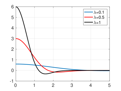
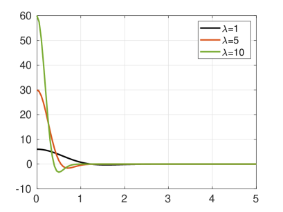
Figure 3.1: Function $G_{3}(r)$ visualized for different values of the parameter $\lambda\in[0.1,10]$.

Figure 3.1 visualizes the share of function $G_{d}(r)$ in (3.1) for $d=3$ depending on different parameters $\lambda\in[0.1,10]$. We can observe the expected behavior: Gaussian with large exponents $\lambda_{k}$ in the RS decomposition of the discretized reference Newton kernel $\mathbf{P}_{R}$ are responsible for the representation of a “singular” part in the Dirac delta, while the terms with small $\lambda_{k}$ serve for recovering the “nonlocal” part, that should vanish after full summation over indices $k=1,\ldots,M$.

3.2 RS decomposition of the discretized Dirac delta

The idea of the RS decomposition is to modify the right-hand side $\rho_{f}$ in such a way that the short-range part in the solution $u$ can be computed independently and initial equation applies only to its long-range part. The latter is a smooth function, hence the FEM approximation error can be reduced dramatically even on the relatively small grids in 3D.

To fix the idea, we consider the simplest case of the single atom with charge $q=1$ located at the origin, such that $u(x)=\frac{1}{\|x\|}$, $x\in\mathbb{R}^{3}$. Recall that the Newton kernel (2.8) discretized by the $R$-term sum of Gaussians living on the tensor grid $\Omega_{n}$, is represented by a sum of the short- and long-range tensors,

$$\frac{1}{\|x\|}\rightsquigarrow\mathbf{P}_{R}=\mathbf{P}_{R_{s}}+\mathbf{P}_{R_{l}},$$

where

$$\mathbf{P}_{R_{s}}=\sum\limits_{k=R_{l}+1}^{R}{\bf p}^{(1)}_{k}\otimes{\bf p}^{(2)}_{k}\otimes{\bf p}^{(3)}_{k},\quad\mathbf{P}_{R_{l}}=\sum\limits_{k=1}^{R_{l}}{\bf p}^{(1)}_{k}\otimes{\bf p}^{(2)}_{k}\otimes{\bf p}^{(3)}_{k}.$$ (3.2)

Let us consider the formal discrete version of the exact equation for the potential

$$-\Delta\frac{1}{4\pi\|x\|}=\delta(x)$$

by its FD analogy by substitution of $\mathbf{P}_{R}$ instead of $u(x)$ and FEM Laplacian matrix $A_{\Delta}$ instead of $\Delta$. This lead to the grid representation of the Dirac delta

$$\delta(x)\rightsquigarrow\boldsymbol{\delta}_{h}:=-A_{\Delta}\mathbf{P}_{R},$$

which is associated with its differential representation.

Recall that in the case $d=3$ the FEM Laplacian matrix $A_{\Delta}$ takes a form

$$A_{\Delta}=\Delta_{1}\otimes I_{2}\otimes I_{3}+I_{1}\otimes\Delta_{2}\otimes I_{3}+I_{1}\otimes I_{2}\otimes\Delta_{3},$$ (3.3)

where $-\Delta_{\ell}=\frac{1}{h^{2}}\mathrm{tridiag}\{1,-2,1\}\in\mathbb{R}^{n_{\ell}\times n_{\ell}}$, $\ell=1,2,3$, denotes the discrete univariate Laplacian, and $I_{\ell}\in\mathbb{R}^{n_{\ell}\times n_{\ell}}$ is the identity matrix. Here the Kronecker rank of $A_{\Delta}$ equals to $3$.

Then the canonical tensor representation $\boldsymbol{\delta}_{h}$ of the ${\delta}$-function approximated on $n\times n\times n$ Cartesian grid can be computed as the action of the Laplace operator on the Newton kernel given in the canonical rank-$R$ tensor format as follows

$$\boldsymbol{\delta}_{h}=-A_{\Delta}\mathbf{P}_{R}=\sum\limits_{k=1}^{R}\Delta_{1}{\bf p}^{(1)}_{k}\otimes{\bf p}^{(2)}_{k}\otimes{\bf p}^{(3)}_{k}+\sum\limits_{k=1}^{R}{\bf p}^{(1)}_{k}\otimes\Delta_{2}{\bf p}^{(2)}_{k}\otimes{\bf p}^{(3)}_{k}+\sum\limits_{k=1}^{R}{\bf p}^{(1)}_{k}\otimes{\bf p}^{(2)}_{k}\otimes\Delta_{3}{\bf p}^{(3)}_{k}.$$

The above representation was also applied in [4]. Figure 3.2 shows the cross-sections of the Newton kernel and of the Dirac delta computed at the plane $z=0$ using $n\times n\times n$ 3D Cartesian grids with $n=1024$.

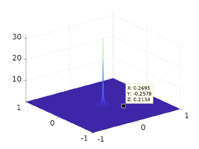
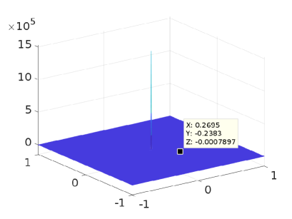
Figure 3.2: The Newton kernel (left) and the Dirac delta (right) computed using the canonical tensor representation on $n\times n\times n$ 3D Cartesian grid with $n=1024$, $R=20$.

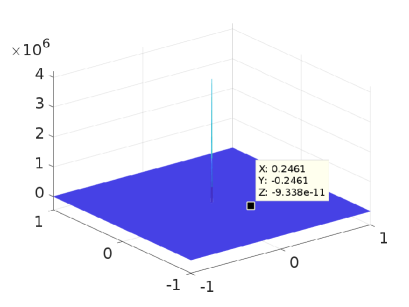
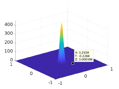
Figure 3.3: Delta function computed by using only short-range (left) and only long-range (right) canonical vectors for $n=1024$, $R=20,R_{l}=12$.

Now we are in a position to construct the RS tensor based splitting scheme. To that end, we introduce the short- and long-range splitting of the discretized $\boldsymbol{\delta}_{h}$ function in the form

$$\boldsymbol{\delta}_{h}=\boldsymbol{\delta}_{s}+\boldsymbol{\delta}_{l},$$

where

$$\boldsymbol{\delta}_{s}:=-A_{\Delta}\mathbf{P}_{R_{s}},\quad\mbox{and}\quad\boldsymbol{\delta}_{l}:=-A_{\Delta}\mathbf{P}_{R_{l}}.$$

Now we observe that by definition the short range part vanishes on the interface $\Gamma$, hence it satisfies the discrete Poisson equation in $\Omega_{m}$ with the respective right-hand side in the form $\boldsymbol{\delta}_{s}$ and zero boundary conditions on $\Gamma$. Then we deduce that this equation can be subtracted from the full discrete linear system, such that the long-range component of the solution, $\mathbf{P}_{R_{l}}$, will satisfy to the same linear system of equations (same interface conditions), but with the right-hand side corresponding to the weighted sum of the long-range tensors $\boldsymbol{\delta}_{l}$ only. In our simple example, we arrive at the particular equation for the long-range part in $\mathbf{P}_{R}$,

$$-A_{\Delta}{\bf u}_{l}=\boldsymbol{\delta}_{l},$$

which, by the construction, recovers the long-range part in the free space harmonic potential.

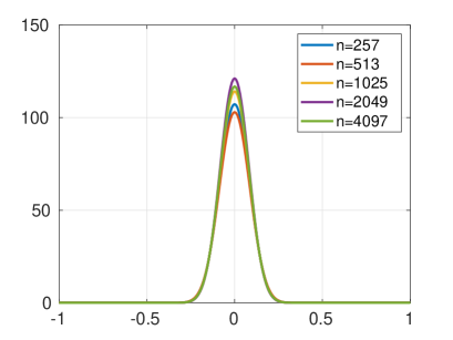
Figure 3.4: The long-range part of the Dirac delta computed using the canonical tensor representation on $n\times n\times n$ 3D Cartesian grid with $n=257,...,4097$, $R=20$.

This scheme can be easily extended to the case of many atomic systems described by (1.4). Let ${\bf P}_{R_{L}}$ be the rank-$R_{L}$ canonical representation of the “long-range part” in the tensor ${\bf P}_{0}$ given by (2.15) and (2.16), obtained by the Can-to-Tuck-to-Can compression scheme [21]. Then the tensor ${\bf P}_{R_{L}}$ can be approximated with controllable accuracy by the solution ${\bf u}_{l,N}\approx{\bf P}_{R_{L}}$ of the discrete Poisson problem with the right-hand side obtained by the $\varepsilon$-adapted rank compression of the $\mbox{rank}\leq 3R_{L}$ tensor $A_{\Delta}{\bf P}_{R_{L}}$,

$$-A_{\Delta}{\bf u}_{l,N}=\boldsymbol{\delta}_{l,N}:=T_{\varepsilon}(\sum\limits_{\nu=1}^{N}\boldsymbol{\delta}_{l,\nu})=-T_{\varepsilon}(A_{\Delta}{\bf P}_{R_{L}}),\quad\boldsymbol{\delta}_{l,\nu}=-A_{\Delta}({z_{\nu}}\,{\cal W}_{\nu}\widetilde{\bf P}_{R_{l}}),$$

where $T_{\varepsilon}$ denotes the operator of the $\varepsilon$-rank truncation. The numerical efficiency of this approach in the case of many-particle systems is based on the important property that the canonical $\varepsilon$-rank of the tensor $\boldsymbol{\delta}_{l,N}$ is almost uniformly bounded in the number of particles $N$ in the system, as proven by the following statement similarly to that in Theorem 2.2, [2, 3]:

Lemma 3.1

Let the long-range part ${\bf P}_{l}$ in the collective interaction potential, see (2.16), correspond to the choice of splitting parameter in (2.14) with $M=O(\log^{2}\varepsilon)$. Then the Tucker $\varepsilon$-rank of the long-range tensor $A_{\Delta}{\bf P}_{R_{L}}\in\mathbb{R}^{n\times n\times n}$ is bounded by

$$|{\bf r}_{0}|:=rank_{Tuck}(A_{\Delta}{\bf P}_{R_{L}})=C_{3}\,b\,\log^{3/2}(|\log(\varepsilon/N)|),$$ (3.4)

where the constant $C_{3}=3C$ does not depend on the number of particles $N$ (here $C$ is the respective constant in (2.18)). The corresponding canonical rank is bounded by $|{\bf r}_{0}|^{2}$.

The tensor $A_{\Delta}{\bf P}_{R_{L}}$ requires $O(|{\bf r}_{0}|^{3}+3|{\bf r}_{0}|\,n)$ numbers to store.

Proof. The proof follows from Theorem 2.2 taking into account that the Kronecker rank of the 3D discrete Laplacian is equal to $3$. The bound on the storage size follows from the rank estimate (3.4).   

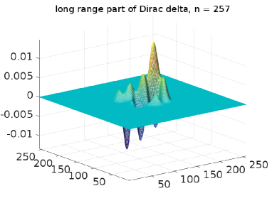
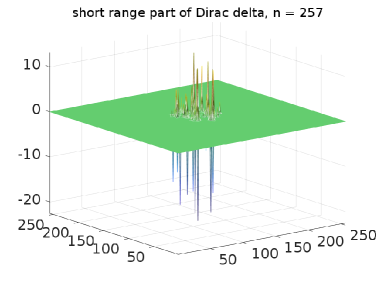
Figure 3.5: The long- and short-range parts of the $N$-particle Dirac delta computed using the canonical tensor representation on $n\times n\times n$ grid with $n=257$, and $N=782$.

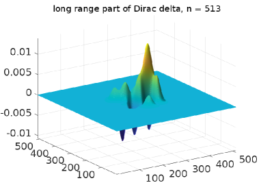
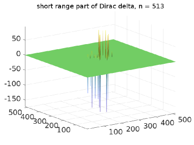
Figure 3.6: The long- and short-range parts of the $N$-particle Dirac delta computed using the canonical tensor representation on $n\times n\times n$ grid with $n=513$, $R=20$, and $N=782$.

Figure 3.4 demonstrates the behavior of the long-range tensor $A_{\Delta}{\bf P}_{R_{L}}$ computed on a sequence of large $n\times n\times n$ 3D Cartesian grids for $n=257,513,\ldots,4097$. We observe that the effective support of this tensor is getting smaller for larger values of the grid size $n$, which that is important for solving elliptic PDEs with heterogeneous data arising in large scale applications (see also §3.3 – §4.3).

Figures 3.5 and 3.6 represent the long- and short-range components of the $N$-particle Dirac delta in the form $\sum\limits_{{k}=1}^{N}q_{k}\delta(\|{x}-{x}_{k}\|)$, corresponding to the protein like neutral molecular system composed of $N=500$ atoms. Similar molecular systems were used in [2, 3] in numerical tests on the RS tensor approximation. The RS tensor representation is implemented on $n\times n\times n$ Cartesian grids with $n=257,513$. We observe that the long-range part remains stable for finer grid, while the short-range part increases with factor for double mesh-size. The canonical rank of the reference potential was set up for $R=24$, with $R_{l}=12$. The Tucker rank of the collective potential is about $R_{Tuck}=30$ which allows the low rank canonical decomposition of the target tensor $\boldsymbol{\delta}_{l,\nu}=-A_{\Delta}({z_{\nu}}{\cal W}_{\nu}\widetilde{\bf P}_{R_{l}})$ by using the can-to-Tuck-to-can rank reduction algorithm [21] applied to the initial rank-$9384$ canonical tensor.

3.3 The linearized Poisson-Boltzmann model

The Poisson-Boltzmann equation (PBE) is the commonly used model for numerical simulation of the 3D electrostatic potential of bio-molecules. The PBE applies to a solvated bio-molecular system modeled by dielectrically separated domains with singular Coulomb potentials distributed in the molecular region. We consider a system embedded into a rectangular domain $\Omega=\overline{\Omega}_{m}\cup\overline{\Omega}_{s}$ with boundary $\partial\Omega$, see Fig. 1.1, where the molecule (solute) region $\Omega_{m}$ is a union of small spheres of radius $\sigma>0$ (Van der Waals sphere of a solute atom) surrounding each individual atom in the system. The solute region is immersed into the the solvent region $\Omega_{s}$.

The linearized Poisson-Boltzmann equation for the electrostatic potential of a bio-molecule, $u(x)$, $x\in\mathbb{R}^{3}$, takes a form, see [12],

$$-\nabla\cdot(\epsilon\nabla u)+\kappa^{2}u=\rho_{f}=\sum\limits_{{k}=1}^{N}q_{k}\delta(\|{x}-{x}_{k}\|)\quad\mbox{in }\quad\Omega\in\mathbb{R}^{3},$$ (3.5)

where $\rho_{f}$ is the scaled singular charge distribution supported at points $x_{k}$ in $\Omega_{m}$, $\delta$ is the Dirac delta, and $q_{k}\in\mathbb{R}$ denotes the charge located at the atomic center $x_{k}$. Here $\epsilon_{m}=O(1)>0$ and $\kappa=0$ in $\Omega_{m}$, while in the solvent region $\Omega_{s}$ we have $\kappa\geq 0$ and $\epsilon_{s}\geq\epsilon_{m}$ (the typical ration $\epsilon_{s}/\epsilon_{m}$ could be about several tens, say, about $80$ for water). Here $\kappa$ is the so-called Debeye length that characterizes the screening effect (due to presence of the ions). The interface conditions on the interior boundary $\Gamma=\partial\Omega_{m}$ arise from the dielectric theory (continuity of potentials and flaxes):

$$[u]=0,\quad\left[\epsilon\frac{\partial u}{\partial n}\right]=0\quad\mbox{on}\quad\Gamma.$$ (3.6)

The boundary conditions on the external boundary are specified depending on the particular problem setting. The simplest choice is either the Dirichlet $u_{|\partial\Omega}=0$ or mixed $\frac{\partial u}{\partial n}=\mu u$ boundary conditions on $\partial\Omega$.

The traditional numerical approaches to PBE are based on either multigrid [12, 26] or domain decomposition [8, 23] methods, combined with certain regularization schemes diminishing the strong singularity in the right-hand side.

In what follows, we briefly sketch the new regularization scheme based on the RS splitting of the discretized Dirac delta described in §3.2. To avoid the unessential technical details, we present the main construction on the continuous level such that our regularization scheme applies in the same way to the FEM discretization of the PBE.

Let $u_{f}=u_{\mbox{\footnotesize short}}+u_{\mbox{\footnotesize long}}$ be the RS splitting of the free space potential generated by the density $\frac{1}{\epsilon_{m}}\rho_{f}$, i.e., satisfying the equation

$$-\epsilon_{m}\Delta u_{f}=\rho_{f}\quad\mbox{in}\quad\mathbb{R}^{3}.$$

This introduces the corresponding RS decomposition of the density $\rho_{f}$ in (3.5) due to the equation

$$-\epsilon_{m}\Delta(u_{\mbox{\footnotesize short}}+u_{\mbox{\footnotesize long}})=\rho_{f}=\rho_{\mbox{\footnotesize short}}+\rho_{\mbox{\footnotesize long}},$$

where

$$\rho_{\mbox{\footnotesize short}}=-\epsilon_{m}\Delta u_{\mbox{\footnotesize short}},\quad\mbox{and}\quad\rho_{\mbox{\footnotesize long}}=-\epsilon_{m}\Delta u_{\mbox{\footnotesize long}}.$$

Now we introduce the new regularization scheme by the RS splitting of the solution $u$ in the form

$$u=u_{\mbox{\footnotesize short}}+\overline{u}_{\mbox{\footnotesize long}},$$

where the component $\overline{u}_{\mbox{\footnotesize short}}$ is precomputed explicitly and stored in the canonical/Tucker tensor format living on the fine Cartesian grid, and the unknown function $\overline{u}_{\mbox{\footnotesize long}}$ satisfies the equation with the modified right-hand side

$$-\nabla\cdot\epsilon\nabla\overline{u}_{\mbox{\footnotesize long}}+\kappa^{2}\overline{u}_{\mbox{\footnotesize long}}=\rho_{\mbox{\footnotesize long}}\quad\mbox{in }\quad\Omega,$$ (3.7)

and equipped with the same interface and boundary conditions as the initial PBE.

We conclude with the following

Lemma 3.2

Let the effective support of the short-range component ${\bf P}_{R_{s}}$ in the reference potential ${\bf P}_{R}$ be chosen not larger than $\sigma>0$ (the radius of Van der Waals spheres), then:

(A) the interface conditions in the regularized formulation of the PBE in (3.7) remain the same as in the initial formulation.

(B) The effective support of the modified right-hand side in (3.7) is included into $\Omega_{m}$.

Proof. (A). Since $u_{\mbox{\footnotesize short}}$ is localized within each sphere $S_{k}$ of radius $\sigma$ centers at $x_{k}$ (i.e., $u_{\mbox{\footnotesize short}}$ and its co-normal derivative both vanish on $\Gamma$), we deduce that $\overline{u}_{\mbox{\footnotesize long}}=u-u_{\mbox{\footnotesize short}}$ inherits the same interface conditions on $\Gamma$ as the solution $u$ of PBE (see also arguments in the proof of Lemma 4.1).

Furthermore, the modified density $\rho_{\mbox{\footnotesize long}}=-\epsilon_{m}\Delta u_{\mbox{\footnotesize long}}$ in the right-hand side in (3.7) is the sum of $N$ functions each localized within the corresponding “Van der Waals region” centered at $x_{k}$. Hence the effective support of $\rho_{\mbox{\footnotesize long}}$ is located withing the molecular region $\Omega_{m}$, which proves item (B).   

For justification of the important property (B), we provide the numerical tests which indicate the decrease of the effective support of the long-range part in the discretized Dirac delta if the corresponding mesh size tends to zero, see Figure 3.4.

The discrete version of the regularization scheme introduced above requires the following calculations:

(A) Computation and storage of $\overline{u}_{\mbox{\footnotesize short}}$ in the RS canonical tensor format living on the fine Cartesian grid.

(B) Computation and storage on the fine Cartesian grid of the modified right-hand side $\rho_{\mbox{\footnotesize long}}$ by application the Discrete Laplacian to the long-range part of the free space potential $u_{\mbox{\footnotesize long}}$.

(C) FEM discretization of the regularized equation (3.7) on a coarse enough grid, where the smooth right-hand side is obtained by the simple interpolation of $\rho_{\mbox{\footnotesize long}}$ from the fine Cartesian grid (where the tensor representation of $\rho_{\mbox{\footnotesize long}}$ was precomputed) onto the coarse FEM mesh.

The advantage of the presented regularized formulation is threefold:

• The absence of singularities in the solution $\overline{u}_{\mbox{\footnotesize long}}$, i.e., the relatively coarse grid provides the accurate FEM solution.

• The localization of the solution splitting into the domain $\Omega_{m}$ only, i.e., the interface and boundary conditions remain unchanged.

• The most singular part in the solution is precomputed with high accuracy and stored in the RS tensor format.

In [4], we test numerically the FEM based computational scheme that allows to implement the presented regularization strategy in the easy and effective way by using the multigrid solver.

4 RS tensor decomposition of the elliptic operator inverse

The equation (1.1) implies the integral representation of the elliptic operator inverse (elliptic resolvent) ${\cal L}^{-1}$ in $\mathbb{R}^{d}$, such that the solution $u(x)$ of the equation

$${\cal L}u=f(x),\quad x\in\mathbb{R}^{d},\quad|u(x)|\to 0\quad\mbox{as}\quad\|x\|\to\infty$$ (4.1)

allows the integral convolution type representation

$$u(x)=({\cal L}^{-1}f)(x)=\int_{\mathbb{R}^{d}}p(\|x-y\|)f(y)dy,$$ (4.2)

for integrable, compactly supported density $f$ in the right-hand side, where $p(\|x\|)$ is the the fundamental solution of the elliptic operator ${\cal L}$, satisfying the equation (1.1). Assume that we are given the RS type splitting of the fundamental solution $p(\|x\|)=p_{s}(\|x\|)+p_{l}(\|x\|)$ in (1.2), then we are able to introduce the RS decomposition of the elliptic operator inverse

$${\cal L}^{-1}={\cal L}^{-1}_{s}+{\cal L}^{-1}_{l},$$

where the local ${\cal L}^{-1}_{s}$ and the long-range ${\cal L}^{-1}_{l}$ components of ${\cal L}^{-1}$ are defined by using (4.2),

$$u(x)=({\cal L}^{-1}f)(x)=\int_{\mathbb{R}^{d}}(p_{s}(\|x-y\|)+p_{l}(\|x-y\|))f(y)dy\equiv u_{s}+u_{l},$$ (4.3)

such that

$$u_{s}=\int_{\mathbb{R}^{d}}p_{s}(\|x-y\|)f(y)=:{\cal L}^{-1}_{s}f,\quad u_{l}=\int_{\mathbb{R}^{d}}p_{l}(\|x-y\|)f(y)=:{\cal L}^{-1}_{l}f.$$

This local-global splitting of the elliptic solution operator essentially relies on the RS decomposition of the Green kernel, which can be derived for the wide class of elliptic operators, as demonstrated in the following sections.

The new regularization scheme for the elliptic operator inverse allows to simplify the solution methods for PDEs with piecewise constant coefficients and highly non-regular right-hand sides by introducing the solution decomposition (regularization) $u=u_{s}+\widehat{u}$, where $u_{s}$ can be easily precomputed and the updated right-hand side in the equation for the new unknown function $\widehat{u}$ remains smooth. We explain this regularization scheme in the more detail on the example in §4.1.

4.1 The Poisson problem with localized right-hand side

As a simple example, we show how the RS tensor decomposition of the discretized Newton kernel by (2.11) can be directly applied to the solution of Poisson problem

$$-\Delta\widehat{u}=f,\quad\mbox{in}\quad\Omega\in\mathbb{R}^{3},$$ (4.4)

where $f\in L_{loc}^{2}(\mathbb{R}^{3})$ is the non-regular function with compact support restricted into a subdomain of complicated geometry embedded in $\Omega$ with $\Gamma=\partial\Omega$. In particular, $f$ may by defined on lower dimensional manifold.

For the ease of exposition, in what follows we first describe the idea on the continuous level. Notice that every RS splitting of the Newton kernel $1/\|x\|=p_{s}(\|x\|)+p_{l}(\|x\|)$ generates the corresponding decomposition of the free space solution $u(x)$ in $\mathbb{R}^{3}$, satisfying (4.1) with ${\cal L}=-\Delta$,

$${u}(x)=\int_{\mathbb{R}^{3}}(p_{s}(\|x-y\|)+p_{l}(\|x-y\|))f(y)dy={u}_{s}+{u}_{l}.$$

Here the short-range part

$${u}_{s}=\int_{\mathbb{R}^{3}}p_{s}(\|x-y\|)f(y)dy=(-\Delta)_{s}^{-1}f$$

can be calculated on a grid by direct convolution transform with strongly localized convolving kernel $p_{s}(\|x\|)$ and, hence, has almost the same support as the right-hand side $f$ (i.e., it remains well localized), while the function ${u}_{l}$ has the improved regularity.

Now, we represent the solution of (4.4) in the form

$$\widehat{u}={u}_{s}+\bar{u},$$

where $\bar{u}$ satisfies the Poisson equation with the modified right-hand side $\bar{f}=f+\Delta{u}_{s}$,

$$-\Delta\bar{u}=\bar{f}=f+\Delta{u}_{s}=(I-{\cal L}{\cal L}^{-1}_{s})f\quad\mbox{in}\quad\Omega\in\mathbb{R}^{3},$$ (4.5)

and with the same boundary conditions on $\Gamma$ as the initial equation (4.4).

Lemma 4.1

Suppose that

$$\mbox{dist}(\mbox{supp}f,\Gamma)>\sigma,$$

where $\sigma>0$ denotes the effective support of the short-range part ${\bf P}_{R_{s}}$ in the tensor representation of the Newton kernel, then:
(A) The trace of the regularized solution $\bar{u}$ and its normal derivatives on $\Gamma$ coincide with those for the solution $\widehat{u}$ of the equation (4.4).
(B) The support of the modified right-hand side $\bar{f}$ is strongly embedded into $\Omega$.
(C) The function $\bar{u}$ has as many partial derivatives in the $\sigma$-vicinity of the domain $\mbox{supp}(f)$, as the the long-range part of the Green kernel, $p_{l}(\|x\|)$.

Proof. Indeed, the statement (A) is a consequence of the fact that $u_{s}=0$ on $\Gamma$ and, moreover, $u_{s}$ vanishes in some vicinity of $\Gamma$ since $\mbox{supp}u_{s}$ is strongly embedded in $\Omega$. Hence, the boundary conditions in the regularized problem (4.5) remain unchanged.

Item (B) follows from the localization property of the function $\Delta{u}_{s}$, which, in turn, is the consequence of the localization of the (discretized) convolving kernel $p_{s}(\|x\|)$, that is $\mbox{diam}(\mbox{supp}\,p_{s})\leq\sigma$, and the relation

$$\mbox{dist}(\mbox{supp}\bar{f},\Gamma)\geq\mbox{dist}(\mbox{supp}f,\Gamma)-\sigma>0.$$

To prove (C), we notice that

$$\frac{\partial^{k}}{\partial x_{k}}u_{l}(x)=\int_{\mathbb{R}^{3}}\frac{\partial^{k}}{\partial x_{k}}p_{l}(\|x-y\|)\,f(y)dy,$$

and, hence, $u_{l}$ has as many partial derivatives as the long-range part of the kernel, $p_{l}(\|x\|)$, which has, in general, high regularity or even it is globally analytic. This feature can be then reconstructed to the function $\bar{u}$ by standards arguments based on the properties of the harmonic extension.   

This scheme also applies to the discrete setting by using the RS tensor splitting of the discrete Newton kernel, ${\bf P}_{R}={\bf P}_{R_{l}}+{\bf P}_{R_{s}}$, represented on fine enough $n\times n\times n$ tensor grid including the computational domain $\Omega$. To that end, we consider the discretized representation of (4.2), which then leads to the discrete version of the above regularization scheme by representing the FEM-Galerkin solution $\widehat{\bf u}$ of (4.4) in the form

$$\widehat{\bf u}={\bf P}_{R_{s}}\ast{\bf f}+\bar{\bf u}.$$ (4.6)

Here the vector $\bar{\bf u}$ satisfies the discrete Poisson equation in $\Omega$ with the modified right-hand side $\bar{\bf f}={\bf f}+\Delta_{h}{\bf P}_{R_{s}}$,

$$-\Delta_{h}\bar{\bf u}=\bar{\bf f},$$ (4.7)

and the same boundary conditions on $\Gamma$ as in the initial equation (4.4). The regularized scheme (4.7) can be applied to the equations with piecewise constant (or even nonlinear) coefficients if $\mbox{supp}(f)$ is embedded onto the subdomain with constant coefficient. The solution process for the equation (4.7) can be implemented in rank structured tensor formats when appropriate.

Finally, we summarize the beneficial properties of the regularization scheme (4.6):

• The right-hand side in the regularized equation has much better regularity compared with the possibly non-regular function $f$.

• The boundary conditions in the regularized equation remain the same as in the initial problem.

• The complexity of the calculation the modified right-hand side (3D convolution with highly localized convolving kernel) is proportional to the number of grid points in the active support of the initial right-hand side $f$.

• Rank structured tensor formats can be applied in the solution process if the geometry of the domain $\Omega$ is appropriate.

In the following sections we recall the examples of classical Green kernels which can be represented in the low-rank RS tensor format.

4.2 Equations with the advection-diffusion operators

Consider the fundamental solution of the advection-diffusion operator ${\cal L}_{d}$ with constant coefficients in $\mathbb{R}^{d}$

$${\cal L}_{d}=-\Delta+2\bar{b}\cdot\nabla+\kappa^{2},\quad\bar{b}\in\mathbb{C}^{d},\quad\kappa\in\mathbb{C}.$$

If $\lambda^{2}=\kappa^{2}+|\bar{b}|^{2}\neq 0$, the the fundamental solution (Green kernel) $\kappa_{\lambda}(x)$ of the operator ${\cal L}_{d}$ takes a form

$$\eta_{\lambda}(x)=\frac{e^{\langle\bar{b},{x}\rangle}}{(2\pi)^{d/2}}\left(\frac{\|{x}\|}{\lambda}\right)^{1-d/2}K_{d/2-1}(\lambda\|{x}\|),\quad x\in\mathbb{R}^{d},$$

where $K_{\nu}$ is the modified Bessel function of the second kind (the Macdonald function) [1]. Here, we use the conventional notation $\langle{y},{z}\rangle=\sum_{\ell=1}^{d}y_{\ell}z_{\ell}$, $\|{z}\|^{2}=\langle{z},{z}\rangle$.

If $\kappa^{2}+|\bar{b}|^{2}=0$, then for $d\geq 3$ it holds

$$\eta_{0}(x)=\frac{1}{(d-2)\omega_{d}}\frac{e^{\langle\bar{b},x\rangle}}{\|x\|^{d-2}},$$

where $\omega_{d}$ is the surface area of the unit sphere in $\mathbb{R}^{d}$. Notice that the radial function $\frac{1}{\|x\|^{d-2}}$ for $d\geq 3$ allows the RS decomposition of the corresponding discrete tensor representation based on the sinc quadrature approximation, which implies the RS representation of the kernel function $\eta_{0}(x)$, since the function $e^{\langle\bar{b},x\rangle}$ is already separable.

In the particular case $\bar{b}=0$, we obtain the fundamental solution of the operator ${\cal L}_{3}=-\Delta+\kappa^{2}$ for $d=3$, also known as the Yukawa (for $\kappa\in\mathbb{R}$) or Helmholtz (for $\kappa\in\mathbb{C}$) Green kernels

$$\eta_{\lambda}(x)=\frac{1}{4\pi}e^{-\kappa\|x\|}/\|x\|,\quad x\in\mathbb{R}^{3}.$$

In the case of Yukawa kernel the tensor representations by using Gaussian sums have been discussed in [22, 19] and implemented in [5].

The Helmholtz equation with $\mbox{Im}\,\kappa>0$ (corresponds to the diffraction potentials) arises in problems of acoustics, electromagnetics and optics. We refer to [27] for the detailed discussion of this class of fundamental solutions. Fast algorithms for the oscillating Helmholtz kernel have been considered in [22] and [6]. However, in this case the construction of the RS tensor decomposition remains an open question.

4.3 Elastic and hydrodynamics potentials in $\mathbb{R}^{3}$

In elasticity theory, linear isotropic and homogeneous elastic problems in whole space $\mathbb{R}^{3}$ are governed by the Lamé system of equations

$$\mu\Delta{u}+(\lambda+\mu)\mbox{grad}\,\mbox{div}{u}={f},$$

where ${u}$ is the displacement vector, ${f}$ is the volume force, $\lambda$ and $\mu$ are the Lamé constants. The solution of the Lamé system is given by the volume potentials in the form of convolution integrals

$$u_{k}(x)=\int_{\mathbb{R}^{3}}\Gamma_{k\ell}(x-{y})f_{\ell}({y})d{y},$$

where $\|\Gamma_{k\ell}\|_{3\times 3}$ is the Kelvin-Somigliana fundamental matrix with

$$\Gamma_{k\ell}(x)=\frac{\lambda+\mu}{8\pi\mu(\lambda+2\mu)}\left(\frac{\lambda+3\mu}{\lambda+\mu}\frac{\delta_{k\ell}}{\|x\|}+\frac{x_{k}x_{\ell}}{\|x\|^{3}}\right).$$

We refer to the monographs [27, 13, 28], where the detailed analysis of these fundamental solutions have been presented.

Remark 4.2

For our discussion it is worth to notice that the radial functions $\frac{1}{\|x\|}$ and $\frac{1}{\|x\|^{3}}$, included in the above representation, allow the low-rank RS tensor decompositions, which can be used for the solution of corresponding equations in non-homogeneous media and with the right-hand side composed of many pointwise singular densities (forces).

In the case of 3D biharmonic operator ${\cal L}=\Delta^{2}$ the fundamental solution reads as

$$p(\|x\|)=-\frac{1}{8\pi}\|x\|,\quad x\in\mathbb{R}^{3}.$$

The hydrodynamic potentials correspond to the linearized classical Navier-Stokes equations

$$\nu\Delta{u}-\mbox{grad}\,p={f},\quad\mbox{div}\,{u}=0,$$

where ${u}$ is the velocity field, $p$ denotes the pressure, and $\nu$ is the constant viscosity coefficient. The solution of the Stokes problem in $\mathbb{R}^{3}$ can be expressed by the hydrodynamic potentials

$$u_{k}(x)=\int\limits_{\mathbb{R}^{3}}\sum\limits^{3}_{\ell=1}\Psi_{k\ell}(x-{y})f_{\ell}({y})\mbox{d}{y},\quad p(x)=\int\limits_{\mathbb{R}^{3}}\langle\Theta(x-{y}),{f})({y})\rangle\mbox{d}{y}$$ (4.8)

with the fundamental solution

$$\Psi_{k\ell}(x)=\frac{1}{8\pi\nu}\left(\frac{\delta_{k\ell}}{\|x\|}+\frac{x_{k}x_{\ell}}{\|x\|^{3}}\right),\quad\Theta(x)=\frac{x}{4\pi\|x\|^{3}},\quad x\in\mathbb{R}^{3}.$$ (4.9)

The existence of the low-rank RS tensor representation for both the biharmonic and the hydrodynamic potential is based on the same argument as in Remark 4.2.

5 Conclusions

The method for the operator dependent RS tensor approximation of the Dirac delta in $\mathbb{R}^{d}$ introduced in this paper allows to represent the discretized $\delta$-function as a sum of the short- and long-range rank-structured tensors. Each of these two tensors reproduces the corresponding parts of the RS tensor representation for the discretized Green kernel associated with the target elliptic operator.

We outline how this method can be applied to solving the potential equations in non-homogeneous media when the density in the right-hand side is given by the large sum of pointwise singular charges. The approach can be utilized in various applications modeled by the elliptic problems with jumping (or even nonlinear) coefficients and non-regular right-hand side as described in Section 4, where the RS splitting of the elliptic operator inverse is introduced.

We show that the tensor approximation of the Dirac delta can be efficiently computed by applying the discretized Laplace operator to the canonical RS tensor representation of the Newton kernel on $n\times n\times n$ 3D Cartesian grid. Due to the RS tensor representation, complexity of this numerical approximation scales as $O(n)$ in a grid size.

Since the rank of the long-range part of the RS tensor representation representing the collective electrostatic potentials of a multi-particle system depends only logarithmically on the number of particles, the same property is inherited by the long-range part of the “collective Dirac delta”. It means that the corresponding computational work for numerical treatment of a multiparticle system increases only linearly-logarithmically in the number of particles.

In this way the approach can be applied to the Poisson-Boltzmann equation modeling the electrostatic potential of a bio-molecule. Other possible applications are based on the RS tensor representation of elastic and hydrodynamics potentials in elasticity problems in $\mathbb{R}^{3}$, as well as of the fundamental solution of advection-diffusion operator with piecewise constant coefficients in $\mathbb{R}^{3}$. The presented regularization scheme also applies to the equations with the continuous density in the right-hand that might have very low regularity and the complicated shape of the effective support (say, electrostatics and magnetostatics).

Acknowledgements. The author would like to thank Dr. Venera Khoromskaia (MPI MiS, Leipzig) for useful discussions and numerical simulations.

References

- [1] M. Abramowitz and I. A. Stegun. Handbook of Mathematical Functions. Dover Publ., New York, 1968.
- [2] P. Benner, V. Khoromskaia and B. N. Khoromskij. Range-separated tensor formats for numerical modeling of many-particle interaction potentials. arXiv:1606.09218v3, p. 1-38, 2016.
- [3] P. Benner, V. Khoromskaia and B. N. Khoromskij. Range-separated tensor format for many-particle modeling. SIAM J. Sci. Comp., 40(2), A1034–A1062, 2018.
- [4] P. Benner, V. Khoromskaia, B. N. Khoromskij, C. Kweyu and M. Stein. Regularization of potential equations with singular source terms using the range-separated tensor format. Manuscript in preparation, 2018.
- [5] C. Bertoglio, and B. N. Khoromskij. Low-rank quadrature-based tensor approximation of the Galerkin projected Newton/Yukawa kernels. Comp. Phys. Comm., 183(4), 904–912, 2012.
- [6] G. Beylkin, Ch. Kurcz and L. Monzón: Fast algorithms for Helmholtz Green’s function. Proc. Roy. Soc., Ser. A (2008) 464, 3301-3326.
- [7] D. Braess. Nonlinear approximation theory. Springer-Verlag, Berlin, 1986.
- [8] E. Cances, Y Maday, and B. Stamm. Domain decomposition for implicit solvation models. J. Chem. Phys., 139 (5), 2013, pp. 054111.
- [9] Ewald P. P. Die Berechnung optische und elektrostatischer Gitterpotentiale. Ann. Phys. 64, 253 -287 (1921).
- [10] I. P. Gavrilyuk, W. Hackbusch and B. N. Khoromskij. Hierarchical Tensor-Product Approximation to the Inverse and Related Operators in High-Dimensional Elliptic Problems. Computing 74 (2005), 131-157.
- [11] W. Hackbusch and B. N. Khoromskij. Low-rank Kronecker product approximation to multi-dimensional nonlocal operators. Part I. Separable approximation of multi-variate functions. Computing 76 (2006), 177-202.
- [12] M. J. Holst. Multilevel methods for the Poisson–Boltzmann equation. Ph.D. Thesis, Numerical Computing group, University of Illinois, Urbana-Champaign, IL, USA, 1994.
- [13] G. C. Hsiao, and W. L. Wendland. Boundary integral equations. Springer, Berlin (2008).
- [14] P. H. Hünenberger and J. A. McCammon. Effect of artificial periodicity in simulations of biomolecules under Ewald boundary conditions: a continuum electrostatics study. Biophys. Chemistry, 78, 1999, pp. 69-88.
- [15] V. Khoromskaia. Black Box Hartree-Fock Solver by the Tensor Numerical Methods. Comp. Methods in Applied Math., vol. 14 (2014) No.1, pp.89-111.
- [16] V. Khoromskaia and B. N. Khoromskij. Grid-based lattice summation of electrostatic potentials by assembled rank-structured tensor approximation. Comp. Phys. Comm., 185 (2014) 3162–3174.
- [17] V. Khoromskaia and B. N. Khoromskij. Fast tensor method for summation of long-range potentials on 3D lattices with defects. Numer. Lin. Algebra Appl., 23:249-271, 2016.
- [18] V. Khoromskaia, D. Andrae, and B. N. Khoromskij. Fast and accurate 3D tensor calculation of the Fock operator in a general basis. Comp. Phys. Comm., 183 (2012) 2392-2404.
- [19] Venera Khoromskaia, and Boris. N. Khoromskij. Tensor Numerical Methods in Quantum Chemistry. Research monograph, De Gruyter, Berlin, 2018.
- [20] B. N. Khoromskij. Structured Rank- Decomposition of Function-related Tensors in . Comp. Meth. Applied Math., 6, (2006), 2, 194-220.
- [21] B. N. Khoromskij and V. Khoromskaia. Multigrid Tensor Approximation of Function Related Arrays. SIAM J. Sci. Comp., 31(4), 3002-3026 (2009).
- [22] Boris N. Khoromskij. Tensor Numerical Methods in Scientific Computing. Research monograph, De Gruyter Verlag, Berlin, 2018.
- [23] F. Lipparini, B. Stamm, E. Cances, Y. Maday, and B. Mennucci. Domain decomposition for implicit solvation models. J. Chem. Theor. Comp., 9 (8), 2013, pp. 3637–3648.
- [24] E.B. Lindgren, A. J. Stace, E. Polack, Y. Maday, B. Stamm and E. Besley. An integral equation approach to calculate electrostatic interactions in many-body dielectric systems. J. Comp. Phys., 371, 2018, pp.712-731.
- [25] A. Litvinenko, D. Keyes, V. Khoromskaia, B. Khoromskij, and H. Matthies. Tucker Tensor analysis of Matérn functions in spatial statistics. Preprint. arXiv:1711.06874, 2017.
- [26] B. Z. Lu, Y. C. Zhou, M. J. Holst and J. A. McCammon. Recent progress in numerical methods for the Poisson-Boltzmann equation in biophysical applications. Commun. Comp. Phys., 3 (5), 2008, pp.973–1009.
- [27] V. Maz’ya, G. Schmidt. Approximate Approximations, Math. Surveys and Monographs, vol. 141, AMS 2007.
- [28] S. A. Sauter and Ch. Schwab. Boundary Element Methods. Springer, 2011.
- [29] A. Smilde, R. Bro, P. Geladi. Multi-way Analysis. Wiley, 2004.
- [30] F. Stenger. Numerical methods based on Sinc and analytic functions. Springer-Verlag, Heidelberg, 1993.