-VAEs can retain label information even at high compression
Abstract
In this paper, we investigate the degree to which the encoding of a -VAE captures label information across multiple architectures on Binary Static MNIST and Omniglot. Even though they are trained in a completely unsupervised manner, we demonstrate that a -VAE can retain a large amount of label information, even when asked to learn a highly compressed representation.
1 Introduction
Our research question can be motivated by the following analogy: imagine a bag filled with 100 balls, only 3 of which are red. Imagine your friend reaches into the bag and “randomly” pulls out 70 balls. If they happened to pull out all 3 of the red balls, you would not be all that surprised (the probability of such an event is 34%, the odds are 2 to 1 against). If they reached in and “randomly” pulled out only 10 balls, but managed to pull out all 3 of the red balls, you should expect your friend cheated and was aware of some property of the balls related to color (the probability of drawing all 3 red balls is 0.1%, or odds of 979 to 1). Do VAEs behave more like the first case or the second?
Variational autoencoders (VAEs) learn compressed representations of their input, akin to selecting just a few balls from the bag as representative of the entire contents of the bag. In the case of VAEs, the compressed representation is constructed with the goal of maximizing the fidelity of the reconstructions of the input from the representation. It is an open question, however, whether the compressed representations show any undue preference for higher-level semantic information (the content of input images, or example, as described by a human). If they do not, VAE compression is analogous to blindly drawing balls from the bag, without preferentially selecting red balls (analogous to higher-level semantic information). More compressed representations would retain less semantic information, and the precise relationship might be expected to be linear. If they do, this should be detectable as a nonlinear relationship between the semantic information retained and the compression rate of the representation, and we might ask by which method the VAE’s are “cheating”, somehow sensing the color (label information) in an otherwise color-blind objective (unsupervised learning).
It was recently shown (Alemi et al., 2018; Burgess et al., 2018) that the -VAE objective generally and the VAE objective specifically can be understood to be variational approximations to a constrained mutual information maximization objective:
| (1) |
The goal is to learn a parametric representation of data that retains salient information while compressing the data as much as possible. This objective, however, does not make any distinction on its own as to what constitutes salient information. In fact, from the information theoretic perspective, any information is salient.
Studies (Landauer, 1986) suggest that when a human looks at a picture, they extract only about a dozen bits into their long term memory. The class label of an MNIST digit, which a human immediately perceives, can be encoded in 3.3 bits. A highly-compressed VAE encoding of a 115-bit binarized MNIST image may or may not contain the 3.3 bits representing the digit. (If it does, it’s akin to drawing just a fraction of the total number of balls in the bag and pulling out all 3 red ones.) This motivates our research question: to what degree do our current approaches to unsupervised learning learn to extract the same compressed set of bits that humans do?
2 Methods
To learn our representations, we use the -VAE objective, interpreted in a representational light (Alemi et al., 2018). The encoder learns a stochastic map from data (with density ) to some representation that minimizes the objective , where is the distortion:
| (2) |
The distortion is defined by the negative log likelihood of a trained variational decoder that attempts to reconstruct the image from the representation. It provides, up to an additive constant a lower bound on the mutual information between our image and our representation.
The rate () gives a variational upper bound on the mutual information retained about the image:
| (3) |
defined by means of the variational marginal (usually called the prior for the VAE when interpreted as a generative model). The rate measures the complexity of the learned representation, measured in bits. As an average KL divergence it denotes how many excess bits would be required to communicate the encodings using an entropic code designed for the variational marginal.
When , the -VAE objective is equivalent to the Evidence Lower Bound (ELBO) of variational inference, in which rate is the KL term and distortion is the likelihood term. See Alemi et al. (2018) for a more thorough explanation of the connection between -VAEs and rate-distortion theory.
To measure the degree to which our representation has captured salient information, we measure the mutual information retained about the labels. To do this, after training our -VAE we separately train a variational classifier to provide a lower bound (up to an additive constant), of the mutual information between our learned representation and the labels, the label distortion ().
| (4) |
We additionally train end-to-end classifiers, both of the simple two layer fully connected network used above, as well as a convolutional network to establish baseline supervised values for . We did a hyperparameter search over filter depths and dropout rates to try to establish a good baseline.
In order to help distinguish how much the unsupervised learning could benefit from gross geometric information contained in the data, we compare to a simple stochastic PCA baseline. We first project the data by means of a truncated PCA down to a small number of dimensions (). From here we inject isotropic Gaussian noise of some magnitude . Assuming the data is now exactly Gaussian under the whitening transformation, the mutual information between the input and the representation can be computed exactly (Polyanskiy & Wu, 2017):
| (5) |
To test how much the VAEs, even if unsupervised might benefit from the inductive biases introduced by the convolutional structure of the encoder, we also measured the obtained from a randomly initialized two layer fully connected neural network as the encoder, as well as a randomly initialized convolutional network. These networks were not trained; we simply used the deterministic encoding produced by the randomly initialized architecture and measured how much information they retained about the labels. Note that this is an uncompressed setting, and so should be expected to retain most of the label information.
We test the effect of different encoder architectures, decoder architectures, and marginal distributions on the degree of class-relevant information that the encodings capture.
3 Experiments and discussion
The initial experimental setup is identical to Alemi et al. (2018), where we trained many different architectures of -VAEs for a wide range of s on the Binary Static MNIST dataset of Larochelle & Murray (2011) as well as Omniglot (Lake et al., 2015). The labels for the Binary Static MNIST dataset were obtained by naive Bayes with respect to original MNIST. We then used a two-layer fully-connected network with ELU activations trained with Adam for 100 epochs with a learning rate of 1e-4, decayed by a factor of 10 every 25 epochs.
For Omniglot we used the same data split as in Burda et al. (2015). This allowed us to test both how much information was retained about the alphabet (a one in 50 classification task) as well as about the individual characters (a one in 1623 classification task).
The baseline convolutional classifier for Binary Static MNIST had five 5x5 convolutional layers of depth 64 followed by a two layer 200 unit fully connected classifier. 2x2 max pooling layers and dropout (at a rate of 30%) were used after layers 3 and 5. For the omniglot alphabet task, the same network was used without dropout and deeper (256) convolutional filters. The omniglot character task used a dropout rate of 10% with depth 64 convolutional filters.
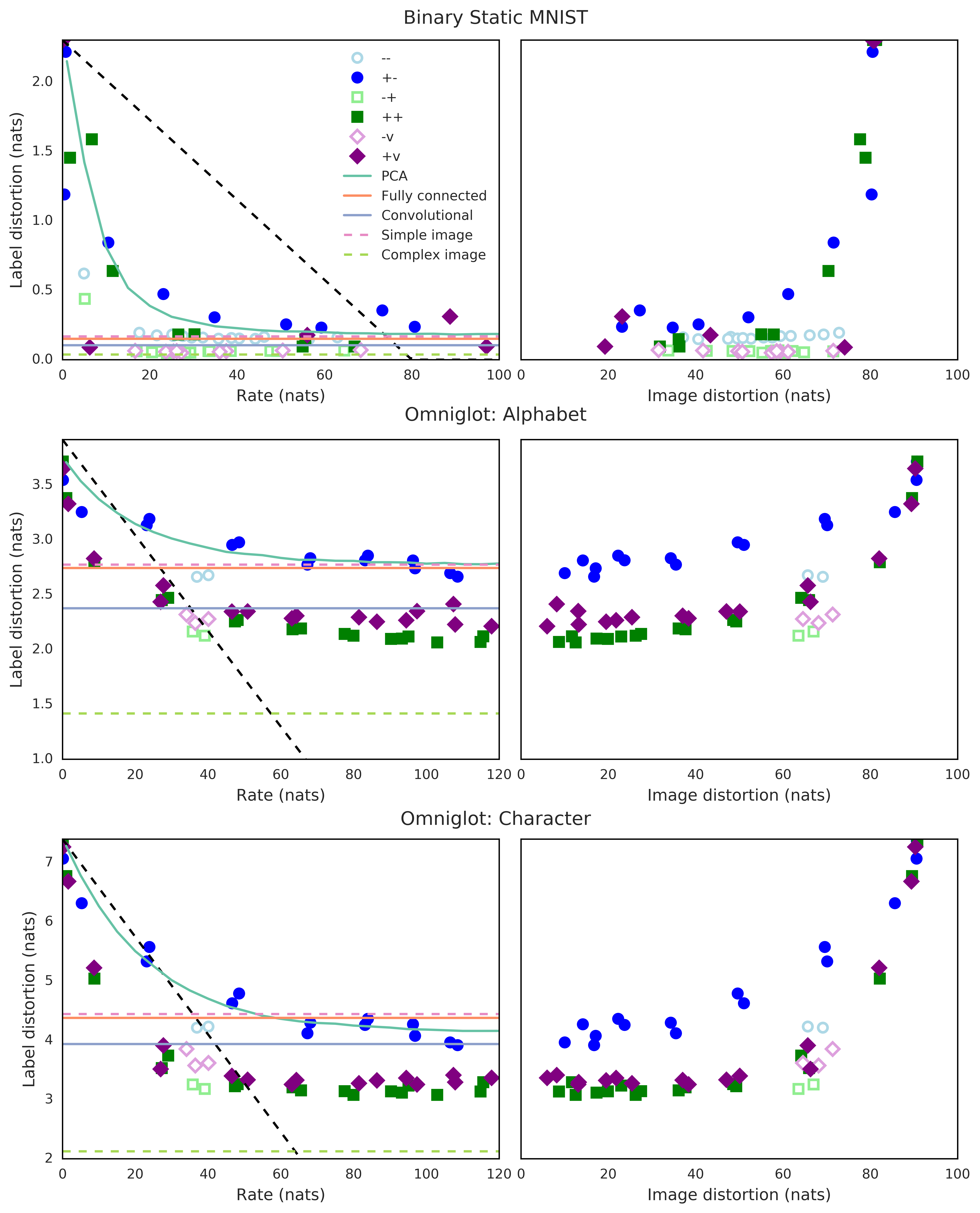
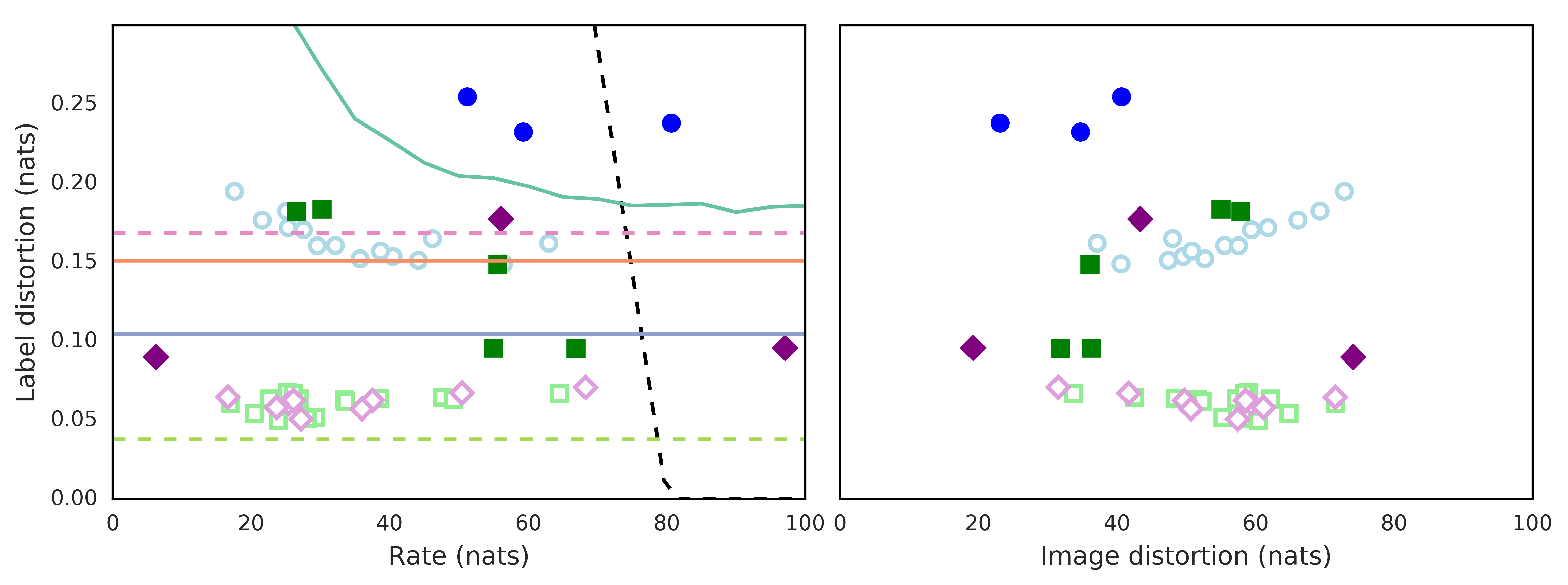
Figure 1 shows the main results. The figures on the left show the measured label distortions () versus rate for all runs and baselines. This shows how much information was retained about the labels (vertical, where lower is better) versus how compressed the representation was (horizontal, left is more compressed). The figures on the right show the label distortion () versus the image distortion (). This shows how much label information is retained versus how well the VAEs were able to reconstruct the original images. A zoomed in version of the MNIST images are shown in Figure 2.
The dashed diagonal black line shows the performance of a method that randomly discards information from an optimal lossless compression (using an estimate of the entropy of 79.78 nats (Tomczak & Welling, 2017)), with no regard for the labels whatsoever. The solid green line (labelled PCA) shows the best randomized PCA results for each dataset (which were a dimensionality of 30 for MNIST and 42 for both Omniglot tasks). The solid red line (Fully connected) shows how much label information was retained in the representation from a randomly initialized fully connected network. The solid blue line (Convolutional) shows how much label information was retained from the activations in a randomly initialized convolutional network. The dashed red line (Simple image) shows the baseline fully trained classifier performance working on the raw images, and lastly the dashed green line (Complex image) shows the fully trained convolutional network’s label distortion. The different network architectures are shown with different symbols.
On MNIST, many runs consistently beat the simple baselines and achieve very small label distortions (, retain a large amount of label information) at small rates (, high compression), showing preference for the label information. Decoder architecture (whether the symbol is solid or open) had a considerable impact on what information the encoder captured: lower label distortions were achieved when a weaker factorized decoder was used rather than the more powerful auto-regressive variant. This is likely because when the decoder is factorized, the mutual information between the latent and each factor has an independent additive effect on the distortion. For a factorized decoder, distortion (up to an additive constant) is:
| (6) |
In the above equation the term measures the gap between the conditional likelihood of each factor () and its variational approximation (i.e the decoder) and the other term () adds the mutual information with the latent for each factor. Consequently, in a low rate setting, the encoder can be biased to capture information that is shared and manifested in more factors (pixels), which our experiments indicate has led to the encoding of more salient features of an image.
On MNIST, (Figure 2) as early as 8 nats in a single instance (which we note used an autoregressive decoder) and around 17 nats generically (for deconvolutional decoders), the -VAEs, were retaining a large amount of label information. They clearly show some preference for label information (i.e. they are much better than the dashed black baseline). Their preference is stronger than can be explained by PCA (solid green line). The inductive biases introduced by convolutional networks seem to be important but we emphasize that the -VAEs were retaining more label information than the random uncompressed convolutional network and within 0.05 nats (0.07 bits) of the most label information able to be extracted even by a fully trained uncompressed network. These baselines are of a different kind than the -VAEs, having unbounded rate.
These -VAE networks, even though there were trained in a completely unsupervised manner and were forced to compress the inputs by a factor of 4 (at a rate near 20), retained nearly all of the label information. In one case, an MNIST -VAE with an autoregressive decoder retained nearly all of the label information at a compression factor over 9.
On the Omniglot Alphabet classification task (second row of Figure 1), the encodings retain much less of the label information. Most of the -VAE points don’t show evidence for preferring the alphabet information (most points are near or to the right of the black dashed line). It is also interesting to note that the autoregressive decoder architectures with the traditional choice of a fixed isotropic Gaussian marginal (prior, solid blue circles) track the randomized PCA baseline. The effect of the prior appears greater for Omniglot than for MNIST, indicating that the Gaussian prior was less able to capture informative encodings for the richer Omniglot dataset. There are a few networks at a rate near 10 that show some preference for alphabet class information, but the effect is much weaker. The -VAEs show more preference for the character identities (third row of Figure 1), but the effect, if still present, is much weaker than on MNIST. This suggests trying much more powerful models on Omniglot to see if the effect can be restored.
4 Conclusion
In conclusion, we have shown that the encodings of a -VAE can capture a significant amount of information that is salient to the class labels, even at high compression rates. This should be surprising given that -VAEs are trained in a completely unsupervised way. The effect is a strong function of decoder architecture, and dataset.
In future work, we plan to test the effect of alternate lower bounds for and , such as those recently proposed in van den Oord et al. (2018); Belghazi et al. (2018). Corroborating our results across multiple lower bounds will strengthen conclusions on the effects of model architecture on . In addition to VAEs, we intend to investigate the extent to which latent representations of other generative models (such as normalizing flows) retain class information. Using the proposed method on richer multiclass datasets, such as CelebA, will enable us to further examine the characteristics of the class labels that are retained in the encodings of different models.
References
- Alemi et al. (2018) Alexander A. Alemi, Ben Poole, Ian Fischer, Joshua V. Dillon, Saurous Rif A., and Kevin Murphy. Fixing a broken elbo. ICML, 2018. URL https://arxiv.org/abs/1711.00464.
- Belghazi et al. (2018) Ishmael Belghazi, Sai Rajeswar, Aristide Baratin, R Devon Hjelm, and Aaron Courville. Mine: mutual information neural estimation. ICML, 2018. URL https://arxiv.org/abs/1801.04602.
- Burda et al. (2015) Yuri Burda, Roger Grosse, and Ruslan Salakhutdinov. Importance weighted autoencoders. 2015.
- Burgess et al. (2018) C. P. Burgess, I. Higgins, A. Pal, L. Matthey, N. Watters, G. Desjardins, and A. Lerchner. Understanding disentangling in -VAE. arXiv, 2018. URL https://arxiv.org/abs/1804.03599.
- Lake et al. (2015) Brenden M. Lake, Ruslan Salakhutdinov, and Joshua B. Tenenbaum. Human-level concept learning through probabilistic program induction. Science, 350(6266):1332–1338, 2015.
- Landauer (1986) Thomas K Landauer. How much do people remember? some estimates of the quantity of learned information in long-term memory. Cognitive Science, 10(4):477–493, 1986.
- Larochelle & Murray (2011) Hugo Larochelle and Iain Murray. The neural autoregressive distribution estimator. 2011.
- Polyanskiy & Wu (2017) Y Polyanskiy and Y Wu. Lecture notes on information theory, 2017. URL http://people.lids.mit.edu/yp/homepage/data/itlectures_v5.pdf.
- Tomczak & Welling (2017) J. M. Tomczak and M. Welling. VAE with a VampPrior. ArXiv e-prints, 2017.
- van den Oord et al. (2018) A. van den Oord, Y. Li, and O. Vinyals. Representation Learning with Contrastive Predictive Coding. arXiv:1807.03748, July 2018. URL https://arxiv.org/abs/1807.03748.