Goodness-of-fit testing the error distribution in multivariate indirect regression

Abstract.

We propose a goodness-of-fit test for the distribution of errors from a multivariate indirect regression model. The test statistic is based on the Khmaladze transformation of the empirical process of standardized residuals. This goodness-of-fit test is consistent at the root-$n$ rate of convergence, and the test can maintain power against local alternatives converging to the null at a root-$n$ rate.

Keywords: hypothesis testing, indirect regression, inverse problems, multivariate regression, regularization

2010 AMS Subject Classifications: Primary: 62G10, 62G30; Secondary: 62G05, 62G08.

1. Introduction

A common problem faced in applications is that one can only make indirect observations of a physical process. Consequently, important quantities of interest cannot be directly observed, but a suitable image under some transformation is typically available. These problems are called inverse problems in the literature. Loosely speaking, the goal is to recover a quantity $\theta$ (often a function) from a distorted version of an image $K\theta$, where $K$ is some operator. Developing valid statistical inference procedures for these inverse problems is desirable, and in recent years several authors have worked on the construction of estimators, structural tests, and (pointwise and uniform) confidence bands for the unknown indirect regression function $\theta$ [see Mair and Ruymgaart (1996), Cavalier and Tsybakov (2002), Johnstone et al. (2004), Bissantz and Holzmann (2008), Cavalier (2008), Birke et al. (2010), Johnstone and Paul (2014), Marteau and Mathé (2014), and Proksch et al. (2015) among many others]. In this paper we consider an indirect regression model of the form

(1.1) $$Y_{j}=\big{[}K\theta\big{]}(X_{j})+\varepsilon_{j},\qquad j=1,\ldots,n,$$

where $X_{j}$ is a predictor, $\varepsilon_{j}$ is a random error and $K$ is a convolution operator, which will be specified later (along with the covariates $X_{j}$). Here $\theta$ is an unknown but square-integrable smooth function. We study a unified approach to testing certain model assumptions regarding the distribution function of the error $\varepsilon_{j}$ in the indirect regression model (1.1).

Apart from specification of the operator $K$, many statistical techniques used in applications for the estimation of $\theta$ depend on the error distribution. For example, when recovering astronomical images certain defects such as cosmic-ray hits are important to identify and remove [Section $6$ of Adorf (1995)]. Here deviation values between observations from pixels and an initial reconstruction are calculated and compared with the standard deviation of the noise. A large deviation indicates the presence of a possible cosmic-ray hit, and observations from the affected pixels are discarded (or replaced by imputed values) in subsequent iterative reconstruction procedures that improve the quality of the final reconstructed image. Determining an unrealistic deviation depends on the structure of the noise distribution. More recently, Bertero et al. (2009) review maximum likelihood methods for reconstruction of distorted images, and, in their Section 5.2 on deconvolution using sparse representation, these authors note the popularity of assuming an additive Gaussian white noise model for transformed data. However, it is not known in advance whether this transformation is appropriate for a given image. If the transformation is inappropriate, then we can expect the Gaussian white noise model to also be inappropriate. The purpose of this paper is to help in answering some of these questions, which could be considered as goodness-of-fit hypotheses of specified error distributions.

Problems of this type have found considerable interest in direct regression models (this is the case where $K$ is an identity operator and only $\theta$ appears in (1.1)) [see Darling (1955), Sukhatme (1972) or Durbin (1973) for some early works or del Barrio et al. (2000) and Khmaladze and Koul (2004) for more recent references]. However, to the best of our knowledge the important case of testing distributional assumptions regarding the error structure of an indirect regression model of the form (1.1) has not been considered so far. We address this problem by proposing a test, which is based on the empirical distribution function of the standardized residuals from an estimate of the regression function. The method is based on a projection principle introduced in the seminal papers of Khmaladze (1981, 1988). This projection is also called the Khmaladze transformation and it has been well-studied in the literature. Exemplarily, we mention the work of Marzec and Marzec (1997), Stute et al. (1998), Khmaladze and Koul (2004, 2009), Haywood and Khmaladze (2008), Dette and Hetzler (2009), Koul and Song (2010), Müller et al. (2012), and Can et al. (2015), who use the Khmaladze transform to construct goodness-fit-tests for various problems. The work which is most similar in spirit to our work is the paper of Koul et al. (2018), who consider a similar problem in linear measurement error models.

We prefer the projection approach because there is a common asymptotic distribution describing the large sample behavior of the test statistics (without unknown parameters to be estimated) and the procedure can be easily adapted to handle different problems. To obtain a better understanding of projection principles as they relate to forming model checks, we direct the reader to consider the rather elaborate work of Bickel et al. (2006), who introduce a general framework for constructing tests of general semiparametric hypotheses that can be tailored to focus substantial power on important alternatives. These authors investigate a so-called score process obtained by a projection principle. Unfortunately, the resulting test statistics are generally not asymptotically distribution free, i.e. the asymptotic distributions of these test statistics generally depend on unknown parameters and inference using them becomes more complicated. The Khmaladze transform is simpler to specify and easily employed in regression problems, since test statistics obtained from the transformation are asymptotically distribution free with (asymptotic) quantiles immediately available.

The article is organized as follows. A brief discussion of Sobolev spaces and their appearance in statistical deconvolution problems is given in Section 2. In this section we further propose an estimator of the indirect regression function and study its statistical properties. The proposed test statistic is introduced in Section 3. Finally, Section 4 concludes the article with a numerical study of the proposed testing procedure and an application. The technical details and proofs of our results can be found in Section 5.

2. Estimating smooth indirect regressions

Consider the model (1.1) with the operator $K$ specifying convolution between an unknown but smooth function $\theta$ and a known distortion function $\psi$ that characterizes $K$, i.e.

(2.1) $$\big{[}K\theta\big{]}(X_{j})=\int_{\mathscr{C}}\theta(\mathbf{u})\psi(X_{j}-\mathbf{u})\,d\mathbf{u}.$$

Here the covariates $X_{j}$ are random and have support $\mathscr{C}=[0,1]^{m}$ for some $m\geq 1$. The model errors $\varepsilon_{1},\ldots,\varepsilon_{n}$ are assumed to be independent with mean zero and common distribution function $F$ admitting a Lebesgue density function, which is denoted by $f$ throughout this paper. We also assume that $\varepsilon_{1},\ldots,\varepsilon_{n}$ are independent of the i.i.d. covariates $X_{1},\ldots,X_{n}$.

Throughout this article we will assume that the indirect regression function $\theta$ from (1.1) is periodic and smooth in the sense that $\theta$ belongs to the subspace of periodic, weakly differentiable functions from the class of square integrable functions $\mathcal{L}_{2}(\mathscr{C})$ with support $\mathscr{C}$; see Chapter 5 of Evans (2010) for definitions and additional discussion. For $d\in\mathbb{N}$ let $I(d)$ be the set of multi-indices $\mathbf{i}=(i_{1},\ldots,i_{m})$ satisfying $\mathbf{i}_{\bullet}=i_{1}+\dots+i_{m}\leq d$. To be precise, we will call a function $q\in\mathcal{L}_{2}(\mathscr{C})$ weakly differentiable in $\mathcal{L}_{2}(\mathscr{C})$ of order $d$ when there is a collection of functions $\{q^{(\mathbf{i})}\in\mathcal{L}_{2}(\mathscr{C})\}_{\mathbf{i}\in I(d)}$ such that

$$\int_{\mathscr{C}}\,q(\mathbf{u})D^{\mathbf{i}}\varphi(\mathbf{u})\,d\mathbf{u}=(-1)^{\mathbf{i}_{\bullet}}\int_{\mathscr{C}}\,q^{(\mathbf{i})}(\mathbf{u})\varphi(\mathbf{u})\,d\mathbf{u},\qquad\mathbf{i}\in I(d),$$

for every infinitely differentiable function $\varphi$, with $\varphi$ and $D^{\mathbf{i}}\varphi$, $\mathbf{i}\in I(d)$, vanishing at the boundary of $\mathscr{C}$ and writing

$$D^{\mathbf{i}}\varphi(\mathbf{x})=\frac{\partial^{\mathbf{i}_{\bullet}}}{\partial x_{1}^{i_{1}}\dots\partial x_{m}^{i_{m}}}\varphi(\mathbf{x}),\qquad\mathbf{x}\in\mathscr{C}.$$

The class of weakly differentiable functions from $\mathcal{L}_{2}(\mathscr{C})$ of order $d$ forms the Sobolev space

$$\mathcal{W}^{d,2}(\mathscr{C})=\bigg{\{}q\in\mathcal{L}_{2}(\mathscr{C})\,:\,q^{(\mathbf{i})}\in\mathcal{L}_{2}(\mathscr{C}),~{}\mathbf{i}\in I(d)\bigg{\}}.$$

The periodic Sobolev space $\mathcal{W}_{\text{per}}^{d,2}$ are those functions from $\mathcal{W}^{d,2}$ that are periodic on $\mathscr{C}$ and whose weak derivatives are also periodic on $\mathscr{C}$. An orthonormal basis for the space $\mathcal{L}_{2}(\mathscr{C})$ of square integrable functions is given by the Fourier basis $\{e^{i2\pi\mathbf{k}\cdot\mathbf{x}}\,:\,\mathbf{x}\in\mathscr{C}\}_{\mathbf{k}\in\mathbb{Z}^{m}}$. Here $\mathbf{k}\cdot\mathbf{x}=k_{1}x_{1}+\dots+k_{m}x_{m}$ is the common inner product between the vectors $\mathbf{k}=(k_{1},\ldots,k_{m})\in\mathbb{Z}^{m}$ and $\mathbf{x}=(x_{1},\ldots,x_{m})\in\mathscr{C}$. It follows that $\mathcal{W}_{\text{per}}^{d,2}$ can be equivalently represented by

$$\mathcal{W}_{\text{per}}^{d,2}=\bigg{\{}q\in\mathcal{W}^{d,2}(\mathscr{C})\,:\,\sum_{\mathbf{k}\in\mathbb{Z}^{m}}\big{(}1+\|\mathbf{k}\|^{2}\big{)}^{d}|\varrho(\mathbf{k})|^{2}<\infty\bigg{\}},$$

where $\|\cdot\|$ denotes the Euclidean norm and

$$\varrho(\mathbf{k})=\int_{\mathscr{C}}\,q(\mathbf{x})e^{-i2\pi\mathbf{k}\cdot\mathbf{x}}\,d\mathbf{x},\quad\mathbf{k}\in\mathbb{Z}^{m}$$

are the Fourier coefficients of $q$ [see Kühn et al. (2014) for further discussion]. The series in the equivalent representation of $\mathcal{W}_{\text{per}}^{d,2}$ motivates replacing the degree of weak differentiability $d$ by a real-valued smoothness index $s>0$. Throughout this article we work with the general indirect regression model space $\mathcal{M}(s)$ defined as

(2.2) $$\mathcal{M}(s)=\bigg{\{}q\in\mathcal{W}_{\text{per}}^{s,2}\,:\,\sum_{\mathbf{k}\in\mathbb{Z}^{m}}\|\mathbf{k}\|^{s}||\varrho(\mathbf{k})|<\infty\bigg{\}}.$$

We will assume that $\theta\in\mathcal{M}(s_{0})$, for some $s_{0}$ specified below, and that $\psi\in\mathcal{L}_{2}(\mathscr{C})$ such that $\psi$ is positive-valued and integrates to $1$ so that $K$ is a convolution operator from $\mathcal{L}_{2}(\mathscr{C})$ into $\mathcal{L}_{2}(\mathscr{C})$. In this case we can represent $K\theta$ in terms of a Fourier series

(2.3) $$K\theta(\mathbf{x})=\sum_{\mathbf{k}\in\mathbb{Z}^{m}}R(\mathbf{k})\exp\big{(}i2\pi\mathbf{k}\cdot\mathbf{x}\big{)}=\sum_{\mathbf{k}\in\mathbb{Z}^{m}}\Psi(\mathbf{k})\Theta(\mathbf{k})\exp\big{(}i2\pi\mathbf{k}\cdot\mathbf{x}\big{)},\qquad\mathbf{x}\in\mathscr{C},$$

where $\{R(\mathbf{k})\}_{\mathbf{k}\in\mathbb{Z}^{m}}$ and $\{\Theta(\mathbf{k})\}_{\mathbf{k}\in\mathbb{Z}^{m}}$ are the Fourier coefficients of $K\theta$ and $\theta$, respectively. In particular we have

(2.4) $$\Theta(\mathbf{k})=\frac{R(\mathbf{k})}{\Psi(\mathbf{k})}\quad\text{for all}~{}\mathbf{k}\in\mathbb{Z}^{m}.$$

Studying the indirect regression model (1.1) requires that we consider the ill-posedness of the inverse problem. This phenomenon occurs because the ratio $|R(\mathbf{k})|/|\Psi(\mathbf{k})|$ needs to be summable when $\theta\in\mathcal{M}(s)$. However, when estimated Fourier coefficients $\{\hat{R}(\mathbf{k})\}_{\mathbf{k}\in\mathbb{Z}^{m}}$ are used $|\hat{R}(\mathbf{k})|$ does not asymptotically vanish (with increasing $\|\mathbf{k}\|$) due to the stochastic noise from the errors $\varepsilon_{j}$ in model (1.1). Consequently, the ratio $|\hat{R}(\mathbf{k})|/|\Psi(\mathbf{k})|$ is not necessarily summable, and this problem is therefore called ill-posed. We can see that the coefficients $\{\Psi(\mathbf{k})\}_{\mathbf{k}\in\mathbb{Z}^{m}}$ determine the rate at which the ratio $|\hat{R}(\mathbf{k})|/|\Psi(\mathbf{k})|$ expands, and, therefore, the ill–posedness of the inverse problem here is given by the rate of decay in the coefficients $\{\Psi(\mathbf{k})\}_{\mathbf{k}\in\mathbb{Z}^{m}}$ of the distortion function $\psi$. We will assume that the inverse problem is mildly to moderately ill-posed in the sense of Fan (1991):

Assumption 1.

There are finite constants $b\geq 0$, $\gamma>0$ and $0\leq C_{\Psi}<C_{\Psi}^{*}$ such that, for every $\|\mathbf{k}\|>\gamma$, the Fourier coefficients $\{\Psi(\mathbf{k})\}_{\mathbf{k}\in\mathbb{Z}^{m}}$ of the function $\psi$ in (2.1) satisfy $C_{\Psi}\leq\|\mathbf{k}\|^{b}|\Psi(\mathbf{k})|<C_{\Psi}^{*}$.

Under Assumption 1, whenever $\theta\in\mathcal{M}(s_{0})$, for some $s_{0}>0$, it follows that $K\theta\in\mathcal{M}(s_{0}+b)$ from the celebrated convolution theorem for the Fourier transformation. This means that convolution of the indirect regression $\theta$ with the distortion function $\psi$ adds smoothness, and the resulting distorted regression function $K\theta$ is now smoother than $\theta$ by exactly the degree of ill-posedness $b$ of the inverse problem. Note that Assumption 1 is milder than that of Fan (1991) in the sense that we allow the degree of ill-posedness $b=0$ and that the scaled Fourier coefficients can vanish. This covers the case of direct regression models where $K$ is the identity operator, that is $K\theta=\theta$. Further note that we do not have to invert the operator $K$ in order to investigate properties of the error distribution in the indirect regression model (1.1).

Several techniques have been developed in the literature to derive series-type estimators (see, for example, Cavalier, 2008). A popular regularization method to employ is the so-called spectral cut-off method, where an indicator function is introduced in (2.3). For example, the indicator function $\mathbf{1}[\|c_{n}\mathbf{k}\|\leq 1]$ (for some sequence $\{c_{n}\}_{n\geq 1}$ converging to $0$) results in a biased version of $K\theta$:

$$(K\theta)_{n}(\mathbf{x})=\sum_{\mathbf{k}\in\mathbb{Z}^{m}\,:\,\|\mathbf{k}\|\leq c_{n}^{-1}}R(\mathbf{k})\exp\big{(}i2\pi\mathbf{k}\cdot\mathbf{x}),\quad\mathbf{x}\in\mathscr{C}.$$

The proposed estimator is obtained by replacing the coefficients $\{R(\mathbf{k})\}_{\mathbf{k}\in\mathbb{Z}^{m}}$ with consistent estimators $\{\hat{R}(\mathbf{k})\}_{\mathbf{k}\in\mathbb{Z}^{m}}$, which gives

$$\sum_{\mathbf{k}\in\mathbb{Z}^{m}\,:\,\|\mathbf{k}\|\leq c_{n}^{-1}}\hat{R}(\mathbf{k})\exp\big{(}i2\pi\mathbf{k}\cdot\mathbf{x}\big{)},\quad\mathbf{x}\in\mathscr{C},$$

as an estimator of $(K\theta)_{n}$. The sequence of smoothing parameters $\{c_{n}\}_{n\geq 1}$ is chosen such that $K\theta$ is consistently estimated. We can generalize this approach as follows.

Following Politis and Romano (1999) we consider a Fourier smoothing kernel $\Lambda$, where $\Lambda$ is defined to be the Fourier transformation of some smoothing kernel function, say $L_{\Lambda}$. The resulting estimate is then defined by

(2.5) $$\widehat{K\theta}(\mathbf{x})=\sum_{\mathbf{k}\in\mathbb{Z}^{m}}\Lambda(c_{n}\mathbf{k})\hat{R}(\mathbf{k})\exp\big{(}i2\pi\mathbf{k}\cdot\mathbf{x}\big{)},\quad\mathbf{x}\in\mathscr{C}.$$

Another useful observation that Politis and Romano (1999) make is the function $\mathbf{x}\mapsto c_{n}^{-m}L_{\Lambda}(c_{n}^{-1}\mathbf{x})$ has Fourier coefficients $\{\Lambda(c_{n}\mathbf{k})\}_{\mathbf{k}\in\mathbb{Z}^{m}}$. Throughout this paper we will choose $\Lambda$ as follows:

Assumption 2.

The Fourier smoothing kernel $\Lambda$ satisfies $\Lambda(\mathbf{k})=1$, for $\|\mathbf{k}\|\leq 1$, $|\Lambda(\mathbf{k})|\leq 1$, for $\|\mathbf{k}\|>1$, and $\int_{\mathbb{R}^{m}}\,\|\mathbf{u}\||\Lambda(\mathbf{u})|\,d\mathbf{u}<\infty$.

The random covariates $X_{1},\ldots,X_{n}$ from model (1.1) are assumed to be independent with distribution function $G$. For simplicity we will assume that $G$ satisfies the following properties.

Assumption 3.

Let the covariate distribution function $G$ admit a positive Lebesgue density function $g\in\mathcal{L}_{2}(\mathscr{C})$ satisfying $\inf_{\mathbf{x}\in\mathscr{C}}g(\mathbf{x})>0$, $\sup_{\mathbf{x}\in\mathscr{C}}g(\mathbf{x})<\infty$ and that $g\in\mathcal{M}(s)$ for some $s>0$.

The boundedness assumptions taken for $g$ are common in nonparametric regression because these conditions guarantee good performance of nonparametric function estimators. The last condition ensures that the density function $g$ satisfies similar smoothness properties as the indirect regression function $\theta$, which allows us to use a Fourier series technique to specify a good estimator of $g$ (see, for example, Politis and Romano, 1999).

What remains is to define the estimates $\{\hat{R}(\mathbf{k})\}_{\mathbf{k}\in\mathbb{Z}^{m}}$ of the Fourier coefficients $\{R(\mathbf{k})\}_{\mathbf{k}\in\mathbb{Z}^{m}}$ required in the definition (2.5). Observing the representation

$$R(\mathbf{k})=\int_{\mathscr{C}}\,\big{[}K\theta\big{]}(\mathbf{x})e^{-i2\pi\mathbf{k}\cdot\mathbf{x}}\,d\mathbf{x}=E\bigg{[}\frac{Y}{g(X)}e^{-i2\pi\mathbf{k}\cdot X}\bigg{]},\quad\mathbf{k}\in\mathbb{Z}^{m},$$

the covariate density function $g$ must be estimated. For this purpose we the expand the density function $g$ into its Fourier series using the coefficients $\{\phi_{g}(\mathbf{k})\}_{\mathbf{k}\in\mathbb{Z}^{m}}$, with $\phi_{g}(\mathbf{k})=E[\exp(-i2\pi\mathbf{k}\cdot X)]$. Estimators of these coefficients are given by

$$\hat{\phi}_{g}(\mathbf{k})=\frac{1}{n}\sum_{j=1}^{n}e^{-i2\pi\mathbf{k}\cdot X_{j}},\quad\mathbf{k}\in\mathbb{Z}^{m}.$$

From these estimators we then obtain an estimator $\hat{g}$ of the unknown covariate density function $g$, that is

(2.6) $$\hat{g}(\mathbf{x})=\frac{1}{n}\sum_{j=1}^{n}W_{c_{n}}\big{(}\mathbf{x}-X_{j}\big{)},\quad\mathbf{x}\in\mathscr{C},$$

with smoothing weights

(2.7) $$W_{c_{n}}\big{(}\mathbf{x}-X_{j}\big{)}=\sum_{\mathbf{k}\in\mathbb{Z}^{m}}\Lambda(c_{n}\mathbf{k})\exp\Big{\{}i2\pi\mathbf{k}\cdot\big{(}\mathbf{x}-X_{j}\big{)}\Big{\}}.$$

Here (as before) the choice of $\Lambda$ defines the form of the smoothing weights $W_{c_{n}}$. The sequence $\{c_{n}\}_{n\geq 1}$ of smoothing parameters is specified later.

We now propose to estimate the Fourier coefficients $\{R(\mathbf{k})\}_{\mathbf{k}\in\mathbb{Z}^{m}}$ of the distorted regression function $K\theta$ by

$$\hat{R}(\mathbf{k})=\frac{1}{n}\sum_{j=1}^{n}\frac{Y_{j}}{\hat{g}(X_{j})}e^{-i2\pi\mathbf{k}\cdot X_{j}},\quad\mathbf{k}\in\mathbb{Z}^{m},$$

where the density estimator $\hat{g}$ is specified in (2.6). This gives for the nonparametric Fourier series estimator in (2.5) the representation

(2.8) $$\widehat{K\theta}(\mathbf{x})=\sum_{\mathbf{k}\in\mathbb{Z}^{m}}\Lambda(c_{n}\mathbf{k})\hat{R}(\mathbf{k})e^{i2\pi\mathbf{k}\cdot\mathbf{x}}=\frac{1}{n}\sum_{j=1}^{n}\frac{Y_{j}}{\hat{g}(X_{j})}W_{c_{n}}\big{(}\mathbf{x}-X_{j}\big{)},\quad\mathbf{x}\in\mathscr{C},$$

where the smoothing weights $W_{c_{n}}$ are defined in (2.7).

The results of Lemma 2 in Section 5 show that the consistency of the estimated Fourier coefficients $\{\hat{R}(\mathbf{k})\}_{\mathbf{k}\in\mathbb{Z}^{m}}$ is heavily dependent on the consistency of the covariate density estimator $\hat{g}$. This fact motivates our choice of smoothing parameters as

(2.9) $$c_{n}=O\big{(}n^{-1/(2s_{0}+2b+3m)}\log^{1/(2s_{0}+2b+3m)}(n)\big{)}$$

and requiring that the covariate density function $g$ has a smoothness index $s=s_{0}+b+m$ in Assumption 3, where $s_{0}$ is the smoothness index of the function class $\mathcal{M}(s_{0})$ to which $\theta$ belongs, $b$ is the degree of ill-posedness of the inverse problem and $m$ is the dimension of the covariates. Our first result result establishes the uniform consistency of the estimator $\widehat{K\theta}$ in (2.5) and a further technical metric space inclusion property that is useful for working with residual-based empirical processes.

Theorem 1.

Let $\theta\in\mathcal{M}(s_{0})$ for some $s_{0}>0$ and let Assumption 1 hold for some degree of ill-posedness $b\geq 0$. Let Assumption 2 hold for a Fourier smoothing kernel $\Lambda$ that satisfies $\int_{\mathbb{R}^{m}}\,\|\mathbf{u}\|^{\max\{s_{0}+b,1\}}|\Lambda(\mathbf{u})|\,d\mathbf{u}<\infty$. Further let Assumption 3 hold for $s=s_{0}+b+m$ and assume that the errors $\varepsilon_{1},\ldots,\varepsilon_{n}$ have a finite absolute moment of order $\kappa>2$. Choose the smoothing parameter $c_{n}$ as in (2.9). Then

$$\sup_{\mathbf{x}\in\mathscr{C}}\Big{|}\widehat{K\theta}(\mathbf{x})-K\theta(\mathbf{x})\Big{|}=O\big{(}n^{-(s_{0}+b)/(2s_{0}+2b+3m)}\log^{(s_{0}+b)/(2s_{0}+2b+3m)}(n)\big{)},\quad\text{a.s.,}$$

and

$$\widehat{K\theta}-K\theta\in\mathcal{M}_{1}(s_{0}+b),\quad\text{a.s.,}$$

where $\mathcal{M}_{1}(s_{0}+b)$ is the unit ball of the metric space $(\mathcal{M}(s_{0}+b),\,\|\cdot\|_{\infty})$.

3. Goodness-of-fit testing the error distribution

In this section we consider the problem of goodness-of-fit testing of a location-scale distribution of the errors in the indirect regression model (1.1) with convolution operator (2.1). Here the location parameter is the mean of the errors and equal to zero, but the scale parameter is unknown. The null hypothesis is given by

(3.1) $$H_{0}\,:\,\exists\sigma>0\,:\,f(t)=\frac{1}{\sigma}f_{*}\bigg{(}\frac{t}{\sigma}\bigg{)},\quad t\in\mathbb{R},$$

where $f_{*}$ is a specified density function of the standardized error distribution and $\sigma$ is the unknown scale parameter. To simplify notation we write $f_{\sigma}$ for the density function of the standardized errors $Z_{j}=\varepsilon_{j}/\sigma$ ($j=1,\ldots,n$) and $F_{\sigma}(t)=\int_{-\infty}^{t}\,f_{\sigma}(y)\,dy$ ($t\in\mathbb{R}$) for the corresponding distribution function. With this notation the null hypothesis in (3.1) becomes $H_{0}\,:\,f_{\sigma}=f_{*}$ for some $\sigma>0$. Equivalently, we can write $H_{0}\,:\,F_{\sigma}=F_{*}$ for some $\sigma>0$ by writing $F_{*}(t)=\int_{-\infty}^{t}\,f_{*}(y)\,dy$ ($t\in\mathbb{R}$) for the error distribution function specified by the null hypothesis.

Following Müller et al. (2012), who consider a similar problem in the direct case, we propose to use the standardized residuals

$$\hat{Z}_{j}=\frac{\hat{\varepsilon}_{j}}{\hat{\sigma}},\quad j=1,\ldots,n,$$

to form a suitable test statistic, where $\hat{\varepsilon}_{j}=Y_{j}-\widehat{K\theta}(X_{j})$ ($j=1,\ldots,n$) are the residuals in the indirect regression model (1.1) obtained for the estimate (2.8) and

$$\hat{\sigma}=\bigg{\{}\frac{1}{n}\sum_{j=1}^{n}\hat{\varepsilon}_{j}^{2}\bigg{\}}^{1/2}$$

is a consistent estimator of the scale parameter $\sigma$. A nonparametric estimator of $F_{*}$ is given by the empirical distribution function of these standardized residuals,

$$\hat{\mathbb{F}}(t)=\frac{1}{n}\sum_{j=1}^{n}\mathbf{1}\big{[}\hat{Z}_{j}\leq t\big{]},\quad t\in\mathbb{R}.$$

The null hypothesis $H_{0}$ is then rejected if a given metric between the estimated standardized distribution function $\hat{\mathbb{F}}$ and $F_{*}$ is large enough. A popular metric in the literature is the supremum metric, and this leads to the Kolmogorov-Smirnov test statistic:

$$\sup_{t\in\mathbb{R}}\Big{|}\hat{\mathbb{F}}(t)-F_{*}(t)\Big{|}.$$

Critical values for the Kolmogorov-Smirnov test statistic are then determined from asymptotic theory, but these can be difficult to work with in practice because they depend on $F_{*}$. To avoid this problem, we will work with a different test statistic.

Our proposed test statistic will crucially depend on the estimator $\hat{\mathbb{F}}$ satisfying an asymptotic expansion, which is given in the following result.

Theorem 2.

Let the assumptions of Theorem 1 hold, with $s_{0}+b>3m/2$ and assume that the Fourier smoothing kernel $\Lambda$ is radially symmetric. Let $F_{*}$ have a finite absolute moment of order $4$ or larger and a bounded Lebesgue density $f_{*}$ that is (uniformly) Hölder continuous with exponent $3m/(2s_{0}+2b)<\gamma\leq 1$. Finally, the function $t\mapsto tf_{*}(t)$ is assumed to be uniformly continuous and bounded. Then under the null hypothesis (3.1)

$$\hat{\mathbb{F}}(t)-F_{*}(t)=\frac{1}{n}\sum_{j=1}^{n}\bigg{\{}\mathbf{1}[Z_{j}\leq t]-F_{*}(t)+f_{*}(t)\bigg{(}Z_{j}+t\frac{Z_{j}^{2}-1}{2}\bigg{)}\bigg{\}}+D_{n}(t),\quad t\in\mathbb{R},$$

with $\sup_{t\in\mathbb{R}}|D_{n}(t)|=o_{P}(n^{-1/2})$.

Remark 1.

A direct consequence of Theorem 2 is that, under the null hypothesis (3.1), the stochastic process $\{\sqrt{n}(\hat{\mathbb{F}}(t)-F_{*}(t))\}_{t\in\mathbb{R}}$ weakly converges in the space $\ell^{\infty}([-\infty,\,\infty])$ to a Gaussian process, which is also the weak limit of the stochastic process

$$\bigg{\{}\frac{1}{\sqrt{n}}\sum_{j=1}^{n}\bigg{\{}\mathbf{1}[Z_{j}\leq t]-F_{*}(t)+f_{*}(t)\bigg{(}Z_{j}+t\frac{Z_{j}^{2}-1}{2}\bigg{)}\bigg{\}}\bigg{\}}_{t\in\mathbb{R}}.$$

This limit distribution can be easily simulated. However, it is clearly not distribution free because it depends on $F_{*}$ and $f_{*}$ specified in the null hypothesis.

In order to obtain a test statistic whose critical values are independent from the distribution specified in the null hypothesis, we use a particular projection of the residual-based empirical process by viewing this quantity as an (approximate) semimartingale with respect to its natural filtration. The projection is given by the Doob-Meyer decomposition of this semimartingale (see page 1012 of Khmaladze and Koul, 2004). For this purpose we will assume that $F_{*}$ has finite Fisher information for location and scale, i.e.

(3.2) $$\int_{-\infty}^{\infty}\big{(}1+t^{2}\big{)}\bigg{(}\frac{f_{*}^{\prime}(t)}{f_{*}(t)}\bigg{)}^{2}\,F_{*}(dt)<\infty,$$

writing $f_{*}^{\prime}$ for the derivative of the Lebesgue density $f_{*}$.

The Khmaladze transformation produces a standard limiting distribution: a standard Brownian motion on $[0,\,1]$, and as a consequence we can construct test statistics which are asymptotically distribution free, i.e. the corresponding critical values do not depend on $F_{*}$ specified by the null hypothesis.

To be precise, note that $F_{*}$ characteristically has mean zero and variance equal to one. In order to introduce our test statistic we define the augmented score function

$$h(t)=(1,-f_{*}^{\prime}(t)/f_{*}(t),-(tf_{*}(t))^{\prime}/f_{*}(t))^{T}$$

and the incomplete information matrix

(3.3) $$\Gamma(t)=\int_{t}^{\infty}\,h(u)h(u)^{T}\,F_{*}(du),\quad t\in\mathbb{R}.$$

Following Khmaladze and Koul (2009) the transformed empirical process of standardized residuals is given by

$$\hat{\xi}_{0}(t)=n^{1/2}\bigg{\{}\hat{\mathbb{F}}(t)-\int_{-\infty}^{t}\,h^{T}(y)\Gamma^{-1}(y)\int_{y}^{\infty}\,h(z)\hat{\mathbb{F}}(dz)\,F_{*}(dy)\bigg{\}},\quad-\infty<t\leq t_{0},$$

for some $t_{0}<\infty$. We can rewrite $\hat{\xi}_{0}$ in a more computationally friendly form, i.e.

$$\hat{\xi}_{0}(t)=n^{1/2}\bigg{\{}\hat{\mathbb{F}}(t)-\frac{1}{n}\sum_{j=1}^{n}\mathscr{G}_{0}\big{(}t\wedge\hat{Z}_{j}\big{)}h\big{(}\hat{Z}_{j}\big{)}\bigg{\}},\quad-\infty<t\leq t_{0},$$

where

$$\mathscr{G}_{0}(t)=\int_{-\infty}^{t}\,h^{T}(y)\Gamma^{-1}(y)\,F_{*}(dy),\quad-\infty<t\leq t_{0}.$$

Under the null hypothesis (3.1) $\hat{\xi}_{0}$ weakly converges in the space $\ell^{\infty}([-\infty,\,t_{0}])$ to $\mathscr{B}(F_{*})$, writing $\mathscr{B}$ for the standard Brownian motion.

In general, the incomplete information matrix $\Gamma$ does not have a simple form, and $\Gamma(t_{0})$ degenerates as $t_{0}\to\infty$. To avoid this degeneracy issue we proceed as in Stute et al. (1998), who recommend using the $99\%$ quantile from the empirical distribution function $\hat{\mathbb{F}}$ for $t_{0}$, i.e. $t_{0}=\hat{\mathbb{F}}^{-1}(0.99)$ writing $\hat{\mathbb{F}}^{-1}$ for the sample quantile function associated with $\hat{\mathbb{F}}$. We propose to base a goodness-of-fit test for the hypothesis (3.1) on the supremum metric between $\hat{\xi}_{0}/(\hat{\mathbb{F}}(t_{0}))^{1/2}$ and the constant $0$:

(3.4) $$T_{0}=\sup_{-\infty<t\leq t_{0}}\bigg{|}\frac{\hat{\xi}_{0}(t)}{(\hat{\mathbb{F}}(t_{0}))^{1/2}}\bigg{|}=\sup_{-\infty<t\leq t_{0}}\bigg{|}\frac{\hat{\xi}_{0}(t)}{0.995}\bigg{|}.$$

The test statistic $T_{0}$ has an asymptotic distribution given by $\sup_{0\leq s\leq 1}|\mathscr{B}(s)|$ under the null hypothesis (3.1).

Our proposed goodness-of-fit test for the null hypothesis (3.1) is then defined by

(3.5) Reject $$H_{0} T_{0}>q_{\alpha}$$ when ,

where $q_{\alpha}$ is the upper $\alpha$-quantile of the distribution of $\sup_{0\leq s\leq 1}|\mathscr{B}(s)|$. The value of $q_{\alpha}$ may be obtained from formula (7) on page 34 of Shorack and Wellner (1986), i.e.

$$P\bigg{(}\sup_{0\leq s\leq 1}\big{|}\mathscr{B}(s)\big{|}>q_{\alpha}\bigg{)}=1-\frac{4}{\pi}\sum_{k=0}^{\infty}\frac{(-1)^{k}}{2k+1}\exp\bigg{(}-\frac{(2k+1)^{2}\pi^{2}}{8q_{\alpha}^{2}}\bigg{)},\quad\alpha<1.$$

For a $5\%$-level test, $\alpha=0.05$ and $q_{0.05}$ is approximately $2.2414$.

4. Finite sample properties

We conclude the article with a numerical study of the previous results with two examples and an application of the proposed test. Throughout this section we consider a goodness-of-fit test for normally distributed errors in the indirect regression model (1.1), i.e.

$$H_{0}\,:\,F_{\sigma}=\Phi\quad\text{for some $\sigma>0$}.$$

Note that in this case a straightforward calculation shows that the augmented score function $h$ and the incomplete information matrix $\Gamma$ from (3.3) become particularly simple, that is $h(t)=(1,\,t,\,t^{2}-1)^{T}$ and

$$\Gamma(t)=\begin{pmatrix}1-\Phi(t)&\phi(t)&t\phi(t)\\ \phi(t)&1-\Phi(t)+t\phi(t)&(t^{2}+1)\phi(t)\\ t\phi(t)&(t^{2}+1)\phi(t)&2(1-\Phi(t))+(t^{3}+t)\phi(t)\end{pmatrix},\quad t\in\mathbb{R},$$

writing $\Phi$ and $\phi$ for the respective distribution and density functions of the standard normal distribution.

4.1. Simulation study

In the first example we generate independent bivariate covariates $X_{j}=(X_{1,j},\,X_{2,j})^{T}$ with independent and identically distributed components $X_{1,j}$ and $X_{2,j}$ ($j=1,\ldots,n$) as follows. The common distribution of $X_{1,j}$ and $X_{2,j}$ is characterized by the density function $g(x_{1},\,x_{2})=g_{1}(x_{1})g_{1}(x_{2})$ ($(x_{1},\,x_{2})^{T}\in[0,\,1]^{2}$), which is depicted in the left panel of Figure 1, where

$$g_{1}(x)=1-\frac{\sqrt{2}}{4}\cos(2\pi x)-\frac{\sqrt{2}}{8}\cos(4\pi x),\quad x\in[0,\,1].$$

One can easily verify that $g$ is a probability density function and satisfies the requirements of Assumption 3 for any $s>0$. The random sample of covariates $X_{1},\ldots,X_{n}$ is then generated from the distribution characterized by the non-trivial density function $g$ using a standard probability integral transform approach. In the second example we use independently, uniformly distributed covariates in the unit square $[0,\,1]^{2}$.

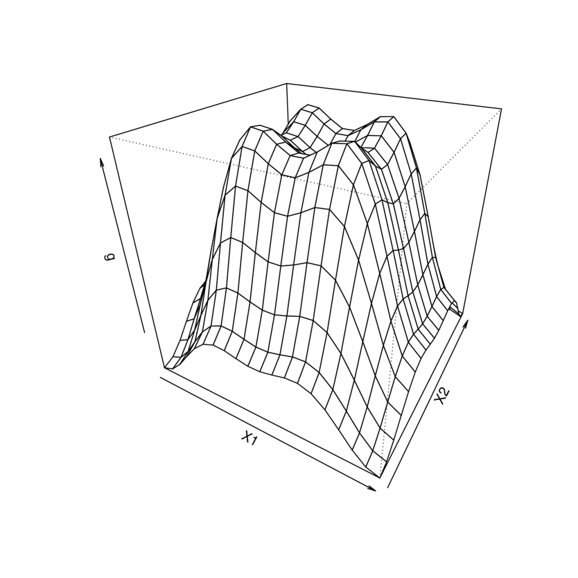
(a)

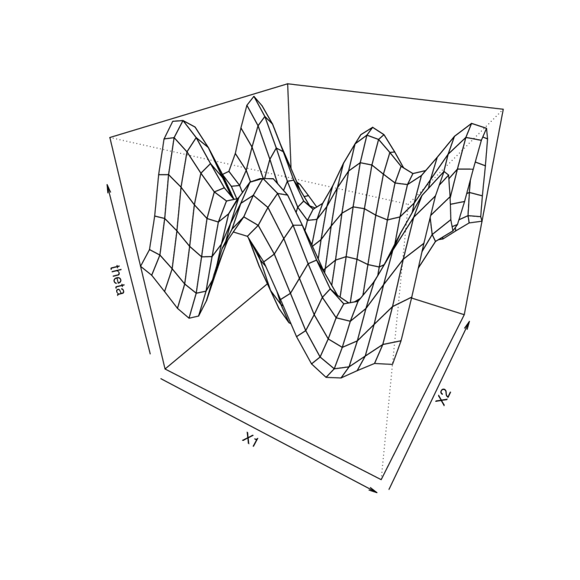
(b)

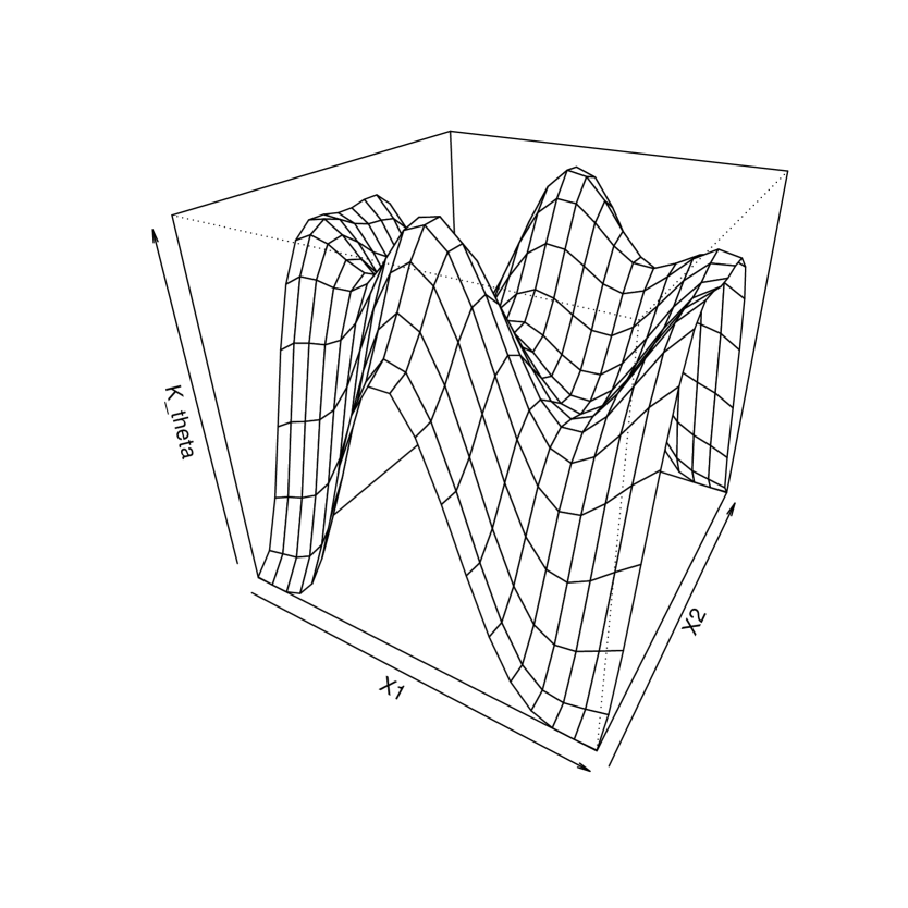
(c)

Figure 1. Perspective plots of (a) the density function $g$, (b) the indirect regression function $\theta$ and (c) the distorted regression function $K\theta$.

The distortion function $\psi$ is taken as the product of two (normalized) Laplace density functions restricted to the interval $[0,\,1]$, each with mean $1/2$ and scale $1/10$. For greater transparency, the Fourier coefficients of the distortion function $\psi$ are

$$\Psi(\mathbf{k})=\frac{\big{(}(-1)^{|k_{1}|}-\exp(-5)\big{)}\big{(}(-1)^{|k_{2}|}-\exp(-5)\big{)}}{(1+4\pi^{2}k_{1}^{2}/10^{2})(1+4\pi^{2}k_{2}^{2}/10^{2})(1-\exp(-5))^{2}},\quad\mathbf{k}=(k_{1},\,k_{2})^{T}\in\mathbb{Z}^{2}.$$

This choice indeed satisfies Assumption 1 with $b=2$. When nonparametric smoothing is performed we work with the radially symmetric spectral cutting kernel characterized by the Fourier coefficient function $\Lambda(c_{n}\mathbf{k})=\mathbf{1}[\|c_{n}\mathbf{k}\|\leq 1]$, $\mathbf{k}\in\mathbb{Z}^{2}$, with smoothing parameter $c_{n}$ chosen by minimizing the leave-one-out cross-validated estimate of the mean squared prediction error (see, for example, Härdle and Marron, 1985). This choice is practical, simple to implement and performed well in our study.

The indirect regression function is given by

$$\theta(x_{1},\,x_{2}) =5+\cos(2\pi x_{1})+\frac{3}{2}\cos(2\pi x_{2})+\frac{3}{2}\cos(4\pi x_{1})$$

$$\quad-2\cos(4\pi x_{2})-2\cos\big{(}2\pi(x_{1}+x_{2})\big{)}-\frac{1}{2}\cos\big{(}2\pi(x_{1}-x_{2})\big{)}$$

for $(x_{1},\,x_{2})^{T}\in[0,\,1]^{2}$. This is easily seen to belong to $\mathcal{M}(s_{0})$ for any $s_{0}>0$. Following the previous discussion, the distorted regression $K\theta$ belongs to $\mathcal{M}(s_{0}+2)$ for any $s_{0}>0$. In the middle and right panels of Figure 1 we display the indirect regression function $\theta$ and the distorted regression function $K\theta$.

	$100$	$200$	$300$	$500$
Normal	$0.048$	$0.098$	$0.072$	$0.052$
Laplace	$0.209$	$0.488$	$0.713$	$0.914$
Skew-normal	$0.136$	$0.388$	$0.577$	$0.828$
Student’s $t$	$0.211$	$0.401$	$0.586$	$0.786$

Table 1. Simulated power of the goodness-of-fit test (3.5) for normally distributed errors at the $5\%$ level with sample sizes $100$, $200$, $300$ and $500$ and with covariates having non-trivial distribution characterized by the density function $g$. The first row corresponds to N$(0,\,(1/2)^{2})$ distributed errors. The remaining rows display the powers of the test under the fixed alternative error distributions: Laplace with scale parameter $\sigma=1/2$; centered, skew-normal with scale parameter $\sigma=1$ and skew parameter $\alpha=3$; Student’s $t$ with $\nu=6$ degrees of freedom.

	$100$	$200$	$300$	$500$
Normal	$0.039$	$0.033$	$0.032$	$0.048$
Laplace	$0.318$	$0.679$	$0.872$	$0.979$
Skew-normal	$0.226$	$0.558$	$0.740$	$0.943$
Student’s $t$	$0.270$	$0.469$	$0.640$	$0.815$

Table 2. Simulated power of the goodness-of-fit test (3.5) for normally distributed errors at the $5\%$ level with sample sizes $100$, $200$, $300$ and $500$ and with covariates independently, uniformly distributed in $[0,\,1]^{2}$. The first row corresponds to N$(0,\,(1/2)^{2})$ distributed errors. The remaining rows display the powers of the test under the fixed alternative error distributions: Laplace with scale parameter $\sigma=1/2$; centered, skew-normal with scale parameter $\sigma=1$ and skew parameter $\alpha=3$; Student’s $t$ with $\nu=6$ degrees of freedom.

We considered four scenarios: normally distributed errors with standard deviation $\sigma=1/2$; Laplace distributed errors with scale parameter $\sigma=1/2$; centered, skew-normal errors with scale parameter $\sigma=1$ and skew parameter $\alpha=3$ (standard deviation is $0.2265$); Student’s $t$ distributed errors with $\nu=6$ degrees of freedom (standard deviation is $1.2247$). The first scenario allows us to check the level of the proposed test statistic $T_{0}$, and the other three scenarios allow for observing the simulated powers of the proposed test. Here we work with a $5\%$-level test, and the quantile $q_{0.05}$ is then $2.2414$.

We perform $1000$ simulation runs of samples of sizes $100$, $200$, $300$ and $500$. Table 1 displays the results for the first example (when the covariates have the non-trivial distribution characterized by the density function $g$) and Table 2 displays the results for the second example (when the covariates are independently, uniformly distributed in the unit square $[0,\,1]^{2}$). Beginning with the first example, at the sample size $100$ the test rejected the null hypothesis in $4.8\%$ of the cases (near the desired $5\%$) but at the sample sizes $200$ and $300$ the test respectively rejected the null hypothesis in $9.8\%$ and in $7.2\%$ of the cases, which are both above the desired $5\%$ nominal level. However, at the sample size $500$ the test rejected the null hypothesis in $5.2\%$ of the cases, which is (again) near the desired nominal level of $5\%$. We expect that this behavior is due to the data-driven smoothing parameter selection. Interestingly, in the second example the test is slightly conservative at all of the simulated sample sizes (e.g. rejecting $3.2\%$ of the cases at sample size $300$), but with sample size $500$ the test rejected the null hypothesis in $4.8\%$ of the cases (near the nominal level of $5\%$), which coincides with the first example.

Turning our attention now to the power of the test, in the first example, we can see that the test performs well for moderate and larger sample sizes. At the sample size $100$ the test respectively rejected the alternative error distributions Laplace, skew-normal and Student’s $t$ in only $20.9\%$, $13.6\%$ and $21.1\%$ of the cases, but at the sample size $500$ the test respectively rejected the alternative distributions in $91.4\%$, $82.8\%$ and $78.6\%$ of the cases. In the second example, we can see that the power of test dramatically improves with smaller sample sizes (rejecting the alternative distributions in $31.8\%$, $22.6\%$ and $27\%$ of the cases at sample size $100$) with less improvement at larger sample sizes (rejecting the alternative distributions in $97.9\%$, $94.3\%$ and $81.5\%$ of the cases at the sample size $500$). In conclusion it appears that the proposed test statistic $T_{0}$ is an effective tool for testing the goodness-of-fit of a desired error distribution in indirect regression models.

4.2. An application to image reconstruction

Here we illustrate an application of the previous results using the HeLa dataset investigated in Bissantz et al. (2009) and more recently by Bissantz et al. (2016). This data composes an image of living HeLa cells obtained using a standard confocal laser scanning microscope and consists of intensity measurements (numbered values $0,\ldots,255$) on $512\times 512$ pixels giving a total of $262144$ observations, see Figure 2. As noted on page $41$ of Bissantz et al. (2009), these image data are (approximately) Poisson distributed. We therefore apply the Anscombe transformation $Y\mapsto 2(Y+3/8)^{1/2}$ to obtain approximately normally distributed data, and then apply the test (3.5) to check the assumption of normally distributed errors (at the $5\%$ level) from a reconstruction of this image using the previously studied results. We use the computing language R with the package OpenImageR, which allows for reading the image data and conducting our analysis.

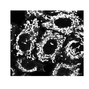
Figure 2. HeLa image data rendered in grayscale.

Since the total number of observations is quite large, we rather illustrate the test for normal errors using two smaller sections of the original HeLa image. To display the reconstructions of the smaller images (for visual comparison with the original data) we apply the inverse of the Anscombe transformation to the fitted values of each regression. In both examples, the pixels are mapped to midpoints of appropriate grids of the unit square $[0,\,1]^{2}$. The first image we consider is $32\times 32$ pixels composing $1024$ observations and is displayed in Figure 3 alongside its reconstructed version and a normal QQ-plot of the resulting standardized regression residuals (see Section 3). The second image we consider is $64\times 64$ pixels composing $4096$ observations and is displayed in Figure 4 alongside its reconstructed version and a normal QQ-plot of the resulting standardized regression residuals. In both cases, as in Section 4.1, when nonparametric smoothing is applied the smoothing parameter is chosen by minimizing the leave-one-out cross-validated estimate of the mean squared prediction error.

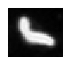
Figure 3. From left to right: $32\times 32$ pixel section of the HeLa image data rendered in grayscale, its reconstructed version (grayscale), a normal QQ-plot of the resulting standardized regression residuals.

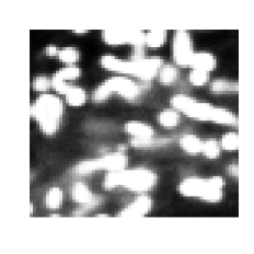
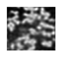
Figure 4. From left to right: $64\times 64$ pixel section of the HeLa image data rendered in grayscale, its reconstructed version (grayscale), a normal QQ-plot of the resulting standardized regression residuals.

Beginning with the first and smaller image, the martingale transform test statistic $T_{0}$ that assesses the goodness-of-fit of a normal distribution has value $1.5141$, which is smaller than $2.2414$, and the null hypothesis of normally distributed errors is not rejected. Inspecting the QQ-plot of these standardized residuals it appears that the assumption of normally distributed errors is appropriate, which confirms our previous finding. In this case, we can see the reconstruction very closely mirrors the original.

Turning now to the second and larger image, the value of the test statistic is $39.8324$, which is much larger than $2.2414$, and we reject the null hypothesis of normally distributed errors. The QQ-plot of the standardized residuals now appears to contain systematic deviation from normality, which confirms that the hypothesis of the normally distributed errors is inappropriate. Here we can see the reconstruction is now not as accurate as it was for the previous case. In conclusion, we can see the approach of using the proposed test statistic $T_{0}$ for assessing convenient forms of the error distribution is useful.

Acknowledgements This work has been supported in part by the Collaborative Research Center “Statistical modeling of nonlinear dynamic processes” (SFB 823, Project C1) of the German Research Foundation (DFG) and in part by the Bundesministerium für Bildung und Forschung through the project “MED4D: Dynamic medical imaging: Modeling and analysis of medical data for improved diagnosis, supervision and drug development”. The authors would also like to thank Kathrin Bissantz for providing us the HeLa cells image used in our data example.

5. Appendix

In this section we give the technical details supporting our results. We have the following uniform convergence property for the density estimator $\hat{g}$.

Lemma 1.

Let the Fourier smoothing kernel $\Lambda$ be as in Assumption 2, and let Assumption 3 hold with $s>0$. Then, for any smoothing parameter sequence $\{c_{n}\}_{n\geq 1}$ satisfying $(nc_{n}^{m})^{-1}\log(n)\to 0$ as $c_{n}\to 0$ with $n\to\infty$,

(5.1) $$\sup_{\mathbf{x}\in\mathscr{C}}\Big{|}\hat{g}(\mathbf{x})-g(\mathbf{x})\Big{|}=O\big{(}c_{n}^{s}+(nc_{n}^{m})^{-1/2}\log^{1/2}(n)\big{)},\quad\text{a.s.}$$

Proof.

Write

$$E\big{[}\hat{g}(\mathbf{x})\big{]}-g(\mathbf{x})=\sum_{\mathbf{k}\in\mathbb{Z}^{m}}\big{\{}\Lambda(c_{n}\mathbf{k})-1\big{\}}\phi_{g}(\mathbf{k})e^{i2\pi\mathbf{k}\cdot\mathbf{x}},\quad\mathbf{x}\in\mathscr{C},$$

(and note that $|\Lambda(c_{n}\mathbf{k})-1|=0$ whenever $\|\mathbf{k}\|\leq c_{n}^{-1}$) to see that

$$\sup_{\mathbf{x}\in\mathscr{C}}\Big{|}E\big{[}\hat{g}(\mathbf{x})\big{]}-g(\mathbf{x})\Big{|}\leq 2c_{n}^{s}\sum_{\mathbf{k}\in\mathbb{Z}^{m}}\|\mathbf{k}\|^{s}|\phi_{g}(\mathbf{k})|=O\big{(}c_{n}^{s}\big{)}.$$

Using the representation $L_{\Lambda}(\mathbf{x})=\sum_{\mathbf{k}\in\mathbb{Z}^{m}}\Lambda(\mathbf{k})e^{i2\pi\mathbf{k}\cdot\mathbf{x}}$ and the fact that $\{\Lambda(c_{n}\mathbf{k})\}_{\mathbf{k}\in\mathbb{Z}^{m}}$ are the Fourier coefficients of the function $L_{\Lambda}(\cdot/c_{n})/c_{n}^{m}$ we obtain

$$\hat{g}(\mathbf{x})-E\big{[}\hat{g}(\mathbf{x})\big{]}=\frac{1}{nc_{n}^{m}}\sum_{j=1}^{n}\bigg{\{}L_{\Lambda}\bigg{(}\frac{\mathbf{x}-X_{j}}{c_{n}}\bigg{)}-E\bigg{[}L_{\Lambda}\bigg{(}\frac{\mathbf{x}-X}{c_{n}}\bigg{)}\bigg{]}\bigg{\}},\quad\mathbf{x}\in\mathscr{C}.$$

One calculates directly that

(5.2) $$\mathrm{Var}\bigg{[}c_{n}^{-m}L_{\Lambda}\bigg{(}\frac{\mathbf{x}-X}{c_{n}}\bigg{)}\bigg{]}=O\big{(}c_{n}^{-m}\big{)},\quad\mathbf{x}\in\mathscr{C}.$$

In addition, $L_{\Lambda}$ is bounded and therefore

(5.3) $$c_{n}^{-m}\sup_{\mathbf{x}\in\mathscr{C}}\bigg{|}L_{\Lambda}\bigg{(}\frac{\mathbf{x}-X_{j}}{c_{n}}\bigg{)}-E\bigg{[}L_{\Lambda}\bigg{(}\frac{\mathbf{x}-X}{c_{n}}\bigg{)}\bigg{]}\bigg{|}=O\big{(}c_{n}^{-m}\big{)},\quad j=1,\ldots,n.$$

To continue, let $\{s_{n}\}_{n\geq 1}$ be a sequence of positive real numbers satisfying $s_{n}=O(c_{n}^{m/2+1})=o(1)$ and partition $\mathscr{C}$ into parts $\mathscr{C}_{i}$ with associated centers $\mathbf{x}_{i}$ ($i=1,\ldots,O(s_{n}^{-m})$) such that $\max_{i=1,\ldots,O(s_{n}^{-m})}\sup_{\mathbf{x}\in\mathscr{C}_{i}}\|\mathbf{x}-\mathbf{x}_{i}\|\leq s_{n}$. The assertion (5.1) follows from the arguments above and by additionally showing that $\max_{i=1,\ldots,O(s_{n}^{-m})}|\hat{g}(\mathbf{x}_{i})-E[\hat{g}(\mathbf{x}_{i})]|=O((nc_{n}^{m})^{-1/2}\log^{1/2}(n))$ and $\max_{i=1,\ldots,O(s_{n}^{-m})}\sup_{\mathbf{x}\in\mathscr{C}_{i}}|\hat{g}(\mathbf{x})-E[\hat{g}(\mathbf{x})]-\hat{g}(\mathbf{x}_{i})+E[\hat{g}(\mathbf{x}_{i})]|=O((nc_{n}^{m})^{-1/2}\log^{1/2}(n))$, almost surely.

Combining (5.2) and (5.3) with Bernstein’s inequality (see, for example, Section 2.2.2 of van der Vaart and Wellner, 1996), one chooses a large enough positive constant $C$ (through the choice of the quantity $O((nc_{n}^{m})^{-1/2}\log^{1/2}(n))$) such that

$$P\bigg{(}\max_{i=1,\ldots,O(s_{n}^{-m})}\big{|}\hat{g}(\mathbf{x}_{i})-E\big{[}\hat{g}(\mathbf{x}_{i})\big{]}\big{|}>O\big{(}(nc_{n}^{m})^{-1/2}\log^{1/2}(n)\big{)}\bigg{)}\leq O\big{(}s_{n}^{-m}n^{-C}\big{)}$$

is summable in $n$. Since $O(s_{n}^{-m}n^{-C})=O((n^{C}c_{n}^{m^{2}/2+m})^{-1})$, this occurs when $C>m/2+2$ and we have

(5.4) $$\max_{i=1,\ldots,O(s_{n}^{-m})}\Big{|}\hat{g}(\mathbf{x}_{i})-E\big{[}\hat{g}(\mathbf{x}_{i})\big{]}\Big{|}=O\big{(}(nc_{n}^{m})^{-1/2}\log^{1/2}(n)\big{)},\quad\text{a.s.}$$

We will now demonstrate that $\max_{\mathbf{k}\in\mathbb{Z}^{m}}|\hat{\phi}_{g}(\mathbf{k})-\phi_{g}(\mathbf{k})|=O(n^{-1/2}\log^{1/2}(n))$, almost surely. Let $\mathbf{k}\in\mathbb{Z}^{m}$ be arbitrary and write

$$\hat{\phi}_{g}(\mathbf{k})-\phi_{g}(\mathbf{k})=\frac{1}{n}\sum_{j=1}^{n}\Big{\{}\exp(i2\pi\mathbf{k}\cdot X_{j})-E\big{[}\exp(i2\pi\mathbf{k}\cdot X)\big{]}\Big{\}},$$

where $X$ is a generic random variable with distribution characterized by the density function $g$. The complex exponential functions are bounded in absolute value by $1$, and it is easy to verify that $\mathrm{Var}[\exp(i2\pi\mathbf{k}\cdot X)]\leq 1$. As above, use Bernstein’s inequality choosing a large enough positive constant $C$ (through the choice of the quantity $O(n^{-1/2}\log^{1/2}(n))$) to find that

$$P\bigg{(}\bigg{|}\frac{1}{n}\sum_{j=1}^{n}\Big{\{}\exp(i2\pi\mathbf{k}\cdot X_{j})-E\big{[}\exp(i2\pi\mathbf{k}\cdot X)\big{]}\Big{\}}\bigg{|}>O\big{(}n^{-1/2}\log^{1/2}(n)\big{)}\bigg{)}\leq O\big{(}n^{-C}\big{)}$$

is summable in $n$. This occurs when $C>1$, independent of $\mathbf{k}$. It follows that $\max_{\mathbf{k}\in\mathbb{Z}^{m}}|\hat{\phi}_{g}(\mathbf{k})-\phi_{g}(\mathbf{k})|=O(n^{-1/2}\log^{1/2}(n))$, almost surely.

Further, let $\mathscr{C}_{i}$ be arbitrary. For any $\mathbf{x}\in\mathscr{C}_{i}$ it follows that

(5.5) $$\hat{g}(\mathbf{x})-E\big{[}\hat{g}(\mathbf{x})\big{]}-\hat{g}(\mathbf{x}_{i})+E\big{[}\hat{g}(\mathbf{x}_{i})\big{]}=\sum_{\mathbf{k}\in\mathbb{Z}^{m}}\Lambda(c_{n}\mathbf{k})\big{\{}\hat{\phi}_{g}(\mathbf{k})-\phi_{g}(\mathbf{k})\big{\}}\Big{\{}e^{i2\pi\mathbf{k}\cdot\mathbf{x}}-e^{i2\pi\mathbf{k}\cdot\mathbf{x}_{i}}\Big{\}}.$$

Now use Euler’s formula to write

$$\exp\big{(}-i2\pi\mathbf{k}\cdot\mathbf{x}\big{)}=\cos\big{(}2\pi\mathbf{k}\cdot\mathbf{x}\big{)}-i\sin\big{(}2\pi\mathbf{k}\cdot\mathbf{x}\big{)},$$

and (using that sine and cosine are Lipschitz functions with constant equal to one) derive the bound

(5.6) $$\Big{|}\exp\big{(}-i2\pi\mathbf{k}\cdot\mathbf{x}\big{)}-\exp\big{(}-i2\pi\mathbf{k}\cdot\mathbf{x}_{i}\big{)}\Big{|}\leq 2^{3/2}\pi\|\mathbf{k}\|\|\mathbf{x}-\mathbf{x}_{i}\|,\quad\mathbf{x}\in\mathscr{C}_{i}.$$

Combining (5.6) with (5.5) there is a positive constant $C>0$ such that

(5.7) $$\max_{i=1,\ldots,O(s_{n}^{-m})}\sup_{\mathbf{x}\in\mathscr{C}_{i}}\Big{|}\hat{g}(\mathbf{x})-E[\hat{g}(\mathbf{x})]-\hat{g}(\mathbf{x}_{i})+E[\hat{g}(\mathbf{x}_{i})]\Big{|}$$

(5.8) $$\leq C(c_{n}^{m+1})^{-1}\max_{\mathbf{k}\in\mathbb{Z}^{m}}\Big{|}\hat{\phi}_{g}(\mathbf{k})-\phi_{g}(\mathbf{k})\Big{|}\max_{i=1,\ldots,O(s_{n}^{-m})}\sup_{\mathbf{x}\in\mathscr{C}_{i}}\|\mathbf{x}-\mathbf{x}_{i}\|\bigg{\{}c_{n}^{m}\sum_{\mathbf{k}\in\mathbb{Z}^{m}}\|c_{n}\mathbf{k}\|\big{|}\Lambda(c_{n}\mathbf{k})\big{|}\bigg{\}}$$

$$=O\big{(}(c_{n}^{m+1})^{-1}s_{n}n^{-1/2}\log^{1/2}(n)\big{)}=O\big{(}(nc_{n}^{m})^{-1/2}\log^{1/2}(n)\big{)},$$

almost surely, since $c_{n}^{m}\sum_{\mathbf{k}\in\mathbb{Z}^{m}}\|c_{n}\mathbf{k}\||\Lambda(c_{n}\mathbf{k})|\to\int_{\mathbb{R}^{m}}\,\|\mathbf{u}\||\Lambda(\mathbf{u})|\,d\mathbf{u}<\infty$ by Assumption 2. ∎

With the results of Lemma 1 we can state a result on the asymptotic order of the estimated coefficients $\{\hat{R}(\mathbf{k})\}_{\mathbf{k}\in\mathbb{Z}^{m}}$, which now depend on the density estimator $\hat{g}$.

Lemma 2.

Let $\theta\in\mathcal{M}(s_{0})$ for some $s_{0}>0$, and assume that the errors $\varepsilon_{1},\ldots,\varepsilon_{n}$ have a finite absolute moment of order $\kappa>2$. Let the Fourier smoothing kernel $\Lambda$ be as in Assumption 2, and let Assumption 3 hold for some $s>0$. Choose the sequence of smoothing parameters $\{c_{n}\}_{n\geq 1}$ such that $(nc_{n}^{m})^{-1}\log(n)\to 0$ and $n^{-1/2}\log^{1/2}(n)=o(c_{n}^{s})$ with $c_{n}\to 0$ as $n\to\infty$. Then

$$\max_{\mathbf{k}\in\mathbb{Z}^{m}}\Big{|}\hat{R}(\mathbf{k})-R(\mathbf{k})\Big{|}=O\big{(}c_{n}^{s}+(nc_{n}^{m})^{-1/2}\log^{1/2}(n)\big{)},\quad\text{a.s.}$$

Proof.

Let $\mathbf{k}\in\mathbb{Z}^{m}$ be arbitrary and write

$$\hat{R}(\mathbf{k})-R(\mathbf{k})=T_{1}(\mathbf{k})+T_{2}(\mathbf{k})+T_{3}(\mathbf{k})+T_{4}(\mathbf{k}),$$

with

$$T_{1}(\mathbf{k})=\frac{1}{n}\sum_{j=1}^{n}\bigg{\{}\frac{[K\theta](X_{j})}{g(X_{j})}e^{-i2\pi\mathbf{k}\cdot X_{j}}-E\bigg{[}\frac{[K\theta](X)}{g(X)}e^{-i2\pi\mathbf{k}\cdot X}\bigg{]}\bigg{\}},$$

$$T_{2}(\mathbf{k})=\frac{1}{n}\sum_{j=1}^{n}\frac{\varepsilon_{j}}{g(X_{j})}e^{-i2\pi\mathbf{k}\cdot X_{j}},$$

$$T_{3}(\mathbf{k})=\frac{1}{n}\sum_{j=1}^{n}\big{[}K\theta\big{]}(X_{j})\Big{\{}\hat{g}^{-1}(X_{j})-g^{-1}(X_{j})\Big{\}}e^{-i2\pi\mathbf{k}\cdot X_{j}}$$

and

$$T_{4}(\mathbf{k})=\frac{1}{n}\sum_{j=1}^{n}\varepsilon_{j}\Big{\{}\hat{g}^{-1}(X_{j})-g^{-1}(X_{j})\Big{\}}e^{-i2\pi\mathbf{k}\cdot X_{j}}.$$

Since $\theta\in\mathcal{M}(s_{0})$ for some $s_{0}>0$, it follows that $K\theta$ is bounded, and a standard argument shows that $\max_{\mathbf{k}\in\mathbb{Z}^{m}}|T_{1}(\mathbf{k})|$ is of the order $O(n^{-1/2}\log^{1/2}(n))=o(c_{n}^{s}+(nc_{n}^{m})^{-1/2}\log^{1/2}(n))$, almost surely. Analogously, $\max_{\mathbf{k}\in\mathbb{Z}^{m}}|T_{2}(\mathbf{k})|$ is of the order $o(c_{n}^{s}+(nc_{n}^{m})^{-1/2}\log^{1/2}(n))$, almost surely. From the result of Lemma 1 we can see that $\max_{\mathbf{k}\in\mathbb{Z}^{m}}|T_{3}(\mathbf{k})|$ is of the order $O(c_{n}^{s}+(nc_{n}^{m})^{-1/2}\log^{1/2}(n))$, almost surely. Finally, with some technical effort one shows that $\max_{\mathbf{k}\in\mathbb{Z}^{m}}|T_{4}(\mathbf{k})|$ is of the order $o(c_{n}^{s}+(nc_{n}^{m})^{-1/2}\log^{1/2}(n))$, almost surely. ∎

We are now ready to state the proof of Theorem 1.

Proof of Theorem 1.

Write

$$\widehat{K\theta}(\mathbf{x})-K\theta(\mathbf{x})=\sum_{\mathbf{k}\in\mathbb{Z}^{m}}\Lambda(c_{n}\mathbf{k})\big{\{}\hat{R}(\mathbf{k})-R(\mathbf{k})\big{\}}e^{i2\pi\mathbf{k}\cdot\mathbf{x}}+\sum_{\mathbf{k}\in\mathbb{Z}^{m}}\big{\{}\Lambda(c_{n}\mathbf{k})-1\big{\}}R(\mathbf{k})e^{i2\pi\mathbf{k}\cdot\mathbf{x}},\quad\mathbf{x}\in\mathscr{C}.$$

From Lemma 2 and that $c_{n}^{s}=O((nc_{n}^{m})^{-1/2}\log^{1/2}(n))$ it follows for the first term in the display above to have the order $O(c_{n}^{s-m})=O(c_{n}^{s_{0}+b})$, almost surely, since $s=s_{0}+b+m$. The second term in the same display is not random and easily shown to be of the order $O(c_{n}^{s_{0}+b})$.

The second assertion follows from showing that $\widehat{K\theta}\in\mathcal{M}(s_{0}+b)$ and combining this fact with the first assertion. The Fourier coefficients of $\widehat{K\theta}$ are given by

$$\Lambda(c_{n}\mathbf{k})\hat{R}(\mathbf{k})=\Lambda(c_{n}\mathbf{k})R(\mathbf{k})+\Lambda(c_{n}\mathbf{k})\big{\{}\hat{R}(\mathbf{k})-R(\mathbf{k})\big{\}},\quad\mathbf{k}\in\mathbb{Z}^{m},$$

and we can see that $|\Lambda(c_{n}\mathbf{k})\hat{R}(\mathbf{k})|$ is bounded by

(5.9) $$|R(\mathbf{k})|+\max_{\xi\in\mathbb{Z}^{m}}\Big{|}\hat{R}(\xi)-R(\xi)\Big{|}|\Lambda(c_{n}\mathbf{k})|.$$

Since $\theta\in\mathcal{M}(s_{0})$ it follows that $\sum_{\mathbf{k}\in\mathbb{Z}^{m}}\|\mathbf{k}\|^{s_{0}+b}|R(\mathbf{k})|=\sum_{\mathbf{k}\in\mathbb{Z}^{m}}\|\mathbf{k}\|^{b}|\Psi(\mathbf{k})|\|\mathbf{k}\|^{s_{0}}|\Theta(\mathbf{k})|<\infty$ and $K\theta\in\mathcal{M}(s_{0}+b)$. This means that we only need to show that the series condition in the definition of $\mathcal{M}(s_{0}+b)$ is satisfied for the second term in (5.9). This series condition results in the quantity

$$\max_{\xi\in\mathbb{Z}^{m}}\Big{|}\hat{R}(\xi)-R(\xi)\Big{|}\sum_{\mathbf{k}\in\mathbb{Z}^{m}}\|\mathbf{k}\|^{s_{0}+b}|\Lambda(c_{n}\mathbf{k})|.$$

We have already used that $\max_{\xi\in\mathbb{Z}^{m}}|\hat{R}(\xi)-R(\xi)|$ is of the order $O(c_{n}^{s})$, and by choice of $\Lambda$ the series in the display above is of the order $O(c_{n}^{-s_{0}-b-m})$ as in the proof of Lemma 1. Combining these findings we can see that the quantity in the display above is of the order $O(c_{n}^{s-s_{0}-b-m})=O(1)$. ∎

The proof of Theorem 2 follows from the above results with an additional property of the distorted regression estimator $\widehat{K\theta}$ and an approximation result for the difference $\hat{\sigma}^{2}-\sigma^{2}$.

Proposition 1.

Choose the Fourier smoothing kernel $\Lambda$ to be radially symmetric. Then the estimator $\widehat{K\theta}$ enjoys the property that

$$\bigg{|}\frac{1}{n}\sum_{j=1}^{n}\Big{\{}\widehat{K\theta}(X_{j})-K\theta(X_{j})\Big{\}}-\frac{1}{n}\sum_{j=1}^{n}\varepsilon_{j}\bigg{|}=0.$$

If the assumptions of Theorem 1 are satisfied with $s_{0}+b>3m/2$, then the estimator $\hat{\sigma}$ enjoys the property that

$$\bigg{|}\hat{\sigma}^{2}-\sigma^{2}-\frac{1}{n}\sum_{j=1}^{n}\big{\{}\varepsilon_{j}^{2}-\sigma^{2}\big{\}}\bigg{|}=o\big{(}n^{-1/2}\big{)},\quad\text{a.s.}$$

Proof.

Write

$$\frac{1}{n}\sum_{j=1}^{n}\Big{\{}\widehat{K\theta}(X_{j})-K\theta(X_{j})\Big{\}}-\frac{1}{n}\sum_{j=1}^{n}\varepsilon_{j}=\frac{1}{n}\sum_{j=1}^{n}Y_{j}\bigg{\{}\frac{\sum_{k=1}^{n}W_{c_{n}}(X_{k}-X_{j})}{\sum_{k=1}^{n}W_{c_{n}}(X_{j}-X_{k})}-1\bigg{\}}.$$

Since $\Lambda$ is radially symmetric, we have that $W_{c_{n}}(X_{j}-X_{k})=W_{c_{n}}(X_{k}-X_{j})$ for every $1\leq j,k\leq n$. One combines this fact with the additional fact that $|Y_{j}|$ is finite with probability 1 for each $1\leq j\leq n$ to finish the proof of the first assertion.

To show the second assertion we need to use the results of Theorem 1 as follows. Write

$$\hat{\sigma}^{2}-\sigma^{2}-\frac{1}{n}\sum_{j=1}^{n}\big{\{}\varepsilon_{j}^{2}-\sigma^{2}\big{\}}=R_{1,n}-2R_{2,n},$$

with

$$R_{1,n}=\frac{1}{n}\sum_{j=1}^{n}\Big{\{}\widehat{K\theta}(X_{j})-K\theta(X_{j})\Big{\}}^{2}$$

and

$$R_{2,n}=\frac{1}{n}\sum_{j=1}^{n}\varepsilon_{j}\Big{\{}\widehat{K\theta}(X_{j})-K\theta(X_{j})\Big{\}}.$$

Now combine the first result of Theorem 1 with $s_{0}+b>3m/2$ to find that $|R_{n,1}|=o(n^{-1/2})$, almost surely.

To continue, write

$$R_{2,n} =\sum_{\mathbf{k}\in\mathbb{Z}^{m}}\big{\{}\Lambda(c_{n}\mathbf{k})-1\big{\}}R(\mathbf{k})\bigg{\{}\frac{1}{n}\sum_{j=1}^{n}\varepsilon_{j}e^{i2\pi\mathbf{k}\cdot X_{j}}\bigg{\}}$$

$$\quad+\sum_{\mathbf{k}\in\mathbb{Z}^{m}}\big{\{}\hat{R}(\mathbf{k})-R(\mathbf{k})\big{\}}\Lambda(c_{n}\mathbf{k})\bigg{\{}\frac{1}{n}\sum_{j=1}^{n}\varepsilon_{j}e^{i2\pi\mathbf{k}\cdot X_{j}}\bigg{\}}$$

to see that $|R_{2,n}|$ is bounded by

$$\max_{\mathbf{k}\in\mathbb{Z}^{m}}\bigg{|}\frac{1}{n}\sum_{j=1}^{n}\varepsilon_{j}e^{i2\pi\mathbf{k}\cdot X_{j}}\bigg{|}\Bigg{[}\max_{\mathbf{k}\in\mathbb{Z}^{m}}\Big{|}\hat{R}(\mathbf{k})-R(\mathbf{k})\Big{|}\sum_{\mathbf{k}\in\mathbb{Z}^{m}}\big{|}\Lambda(c_{n}\mathbf{k})\big{|}+\sum_{\mathbf{k}\in\mathbb{Z}^{m}}\big{|}\Lambda(c_{n}\mathbf{k})-1\big{|}|R(\mathbf{k})|\Bigg{]}.$$

Analogously to the proof of Lemma 2, one treats $\max_{\mathbf{k}\in\mathbb{Z}^{m}}|n^{-1}\sum_{j=1}^{n}\varepsilon_{j}\exp(i2\pi\mathbf{k}\cdot X_{j})|$ using a standard argument and finds this quantity is of the order $O(n^{-1/2}\log^{1/2}(n))$, almost surely. For the quantities inside the large brackets, one uses Lemma 2 and handles the series term as in the proof of Lemma 1 to show that the first term is of the order $O(c_{n}^{s-m})=O(c_{n}^{s_{0}+b})$ (since $s=s_{0}+b+m$) and the second term is easily shown to be of the order $O(c_{n}^{s_{0}+b})$ (see the proof of Lemma 1). Therefore, $|R_{2,n}|$ is of the order $O(c_{n}^{s_{0}+b}n^{-1/2}\log^{1/2}(n))=o(n^{-1/2})$, almost surely. ∎

Neumeyer and Van Keilegom (2010) consider estimation of the distribution function of the standardized errors using a residual-based empirical distribution function based on nonparametric regression residuals obtained by local polynomial smoothing. These authors obtain asymptotic negligibility of a modulus of continuity relating their residual-based empirical distribution function to the empirical distribution function of their regression model errors (see Lemma A.3 in that article). We obtain a similar result for the estimator $\hat{\mathbb{F}}$ (stated as a proposition below) using analogous arguments to those of Neumeyer and Van Keilegom (2010). These arguments have been omitted for brevity.

Proposition 2.

Let the assumptions of Theorem 1 be satisfied with $s_{0}+b>m$. Additionally, assume that $F_{*}$ admits a bounded Lebesgue density $f_{*}$ that satisfies $\sup_{t\in\mathbb{R}}|tf_{*}(t)|<\infty$. Then under the null hypothesis $H_{0}$ in (3.1)

$$\sup_{t\in\mathbb{R}}\bigg{|}\hat{\mathbb{F}}(t)-\frac{1}{n}\sum_{j=1}^{n}F_{*}\bigg{(}t+\frac{\hat{\sigma}-\sigma}{\sigma}t+\frac{\widehat{K\theta}(X_{j})-K\theta(X_{j})}{\sigma}\bigg{)}-\frac{1}{n}\sum_{j=1}^{n}\mathbf{1}[Z_{j}\leq t]+F_{*}(t)\bigg{|}=o_{P}(n^{-1/2}).$$

We are now prepared the state the proof of Theorem 2.

Proof of Theorem 2.

We introduce the notation

$$E_{n}(t)=\frac{1}{n}\sum_{j=1}^{n}\bigg{\{}\mathbf{1}[Z_{j}\leq t]-F_{*}(t)+f_{*}(t)\bigg{(}Z_{j}+t\frac{Z_{j}^{2}-1}{2}\bigg{)}\bigg{\}},\quad t\in\mathbb{R},$$

and write

$$\hat{\mathbb{F}}(t)-F_{*}(t)-E_{n}(t)=M_{n}(t)+H_{n}(t)+L_{n}(t)=D_{n}(t),\quad t\in\mathbb{R},$$

where the remainder term $D_{n}(t)$ is equal to the sum of

$$M_{n}(t)=\hat{\mathbb{F}}(t)-\frac{1}{n}\sum_{j=1}^{n}F_{*}\bigg{(}t+\frac{\hat{\sigma}-\sigma}{\sigma}t+\frac{\widehat{K\theta}(X_{j})-K\theta(X_{j})}{\sigma}\bigg{)}-\frac{1}{n}\sum_{j=1}^{n}\mathbf{1}[Z_{j}\leq t]+F_{*}(t),$$

$$H_{n}(t) =\frac{1}{n}\sum_{j=1}^{n}F_{*}\bigg{(}t+\frac{\hat{\sigma}-\sigma}{\sigma}t+\frac{\widehat{K\theta}(X_{j})-K\theta(X_{j})}{\sigma}\bigg{)}-F_{*}(t)$$

$$\quad-f_{*}(t)\frac{\sigma^{-1}}{n}\sum_{j=1}^{n}\Big{\{}\widehat{K\theta}(X_{j})-K\theta(X_{j})\Big{\}}-tf_{*}(t)\frac{\hat{\sigma}-\sigma}{\sigma},$$

and

$$L_{n}(t)=f_{*}(t)\bigg{\{}\frac{\sigma^{-1}}{n}\sum_{j=1}^{n}\Big{\{}\widehat{K\theta}(X_{j})-K\theta(X_{j})\Big{\}}-\frac{1}{n}\sum_{j=1}^{n}Z_{j}\bigg{\}}+tf_{*}(t)\bigg{\{}\frac{\hat{\sigma}-\sigma}{\sigma}-\frac{1}{n}\sum_{j=1}^{n}\frac{Z_{j}^{2}-1}{2}\bigg{\}}.$$

From Proposition 2 it follows that $\sup_{t\in\mathbb{R}}|M_{n}(t)|=o_{P}(n^{-1/2})$. Proposition 1 in combination with the bounding conditions on $f_{*}$ imply that $\sup_{t\in\mathbb{R}}|L_{n}(t)|=o_{P}(n^{-1/2})$ (note that $Z_{j}=\varepsilon_{j}/\sigma$, $j=1,\ldots,n$).

To show that $\sup_{t\in\mathbb{R}}|H_{n}(t)|=o_{P}(n^{-1/2})$ and finish the proof we need to rewrite $H_{n}(t)=H_{1,n}(t)+H_{2,n}(t)+H_{3,n}(t)$, with $H_{1,n}(t)$ equal to

$$\frac{\sigma^{-1}}{n}\sum_{j=1}^{n}\Big{\{}\widehat{K\theta}(X_{j})-K\theta(X_{j})\Big{\}}\int_{0}^{1}\,\bigg{\{}f_{*}\bigg{(}t+\frac{\hat{\sigma}-\sigma}{\sigma}t+\frac{\widehat{K\theta}(X_{j})-K\theta(X_{j})}{\sigma}s\bigg{)}-f_{*}\bigg{(}t+\frac{\hat{\sigma}-\sigma}{\sigma}t\bigg{)}\bigg{\}}\,ds,$$

$$H_{2,n}(t)=\bigg{\{}f_{*}\bigg{(}t+\frac{\hat{\sigma}-\sigma}{\sigma}t\bigg{)}-f_{*}(t)\bigg{\}}\frac{\sigma^{-1}}{n}\sum_{j=1}^{n}\Big{\{}\widehat{K\theta}(X_{j})-K\theta(X_{j})\Big{\}}$$

and

$$H_{3,n}(t)=\frac{\hat{\sigma}-\sigma}{\sigma}t\int_{0}^{1}\,\bigg{\{}f_{*}\bigg{(}t+\frac{\hat{\sigma}-\sigma}{\sigma}ts\bigg{)}-f_{*}(t)\bigg{\}}\,ds.$$

The Hölder continuity of $f_{*}$ guarantees that

$$\sup_{t\in\mathbb{R}}\big{|}H_{1,n}(t)\big{|}\leq\frac{C_{f_{*}}}{(1+\gamma)\sigma^{1+\gamma}}\sup_{\mathbf{x}\in\mathscr{C}}\Big{|}\widehat{K\theta}(\mathbf{x})-K\theta(\mathbf{x})\Big{|}^{1+\gamma}=o\big{(}n^{-1/2}\big{)},\quad\text{a.s.,}$$

from Theorem 1 and that $3m/(2s_{0}+2b)<\gamma\leq 1$, which is $o_{P}(n^{-1/2})$ and writing $C_{f_{*}}$ for the Hölder constant associated to $f_{*}$. Proposition 1 and the uniform continuity of $f_{*}$ imply that $\sup_{t\in\mathbb{R}}|H_{2,n}(t)|=o_{P}(n^{-1/2})$. Finally, Proposition 1 and the finite fourth moment assumption guarantees that $\hat{\sigma}$ is a root-$n$ consistent estimator of $\sigma$, and combining this fact with the uniform continuity and boundedness of the function $t\mapsto tf_{*}(t)$ implies that $\sup_{t\in\mathbb{R}}|H_{3,n}(t)|=o_{P}(n^{-1/2})$. ∎

References

• [1] Adorf, H.M. (1995). Hubble Space Telescope image restoration in its fourth year. Inverse Problems 11, 639-653.
• [2] Bertero, M., Boccacci, P., Desiderá, G. and Vicidomini, G. (2009). Image deblurring with Poisson data: from cells to galaxies. Inverse Problems 25, 123006.
• [3] Bickel, P.J., Ritov, Y. and Stoker, T.M. (2006). Tailor-made tests for goodness-of-fit to semiparametric hypotheses. Ann. Statist. 34, 721-741.
• [4] Birke, M., Bissantz, N. and Holzmann, H. (2010). Confidence bands for inverse regression models. Inverse Problems 26, 115020.
• [5] Bissantz, N. and Holzmann, H. (2008). Statistical inference for inverse problems. Inverse Problems 24, 034009.
• [6] Bissantz, N., Claeskens, G., Holzmann, H. and Munk, A. (2009). Testing for lack of fit in inverse regression - with applications to biophotonic imaging. J. R. Statist. Soc. B 71, 25-48.
• [7] Bissantz, N., Dette, H., Hildebrandt, T. and Bissantz, K. (2016). Smooth backfitting in additive inverse regression. Ann. Inst. Stat. Math. 68, 827-853.
• [8] Can, S.U., Einmahl, J.H.J., Khmaladze, E.V. and Laeven, R.J.A. (2015). Asymptotically distribution-free goodness-of-fit testing for tail copulas. Ann. Statist. 43, 878-902.
• [9] Cavalier, L. and Tsybakov, A. (2002). Sharp adaptation for inverse problems with random noise. Probab. Theory Relat. Fields 123, 323-354.
• [10] Cavalier, L. (2008). Nonparametric statistical inverse problems. Inverse Problems 24, 034004.
• [11] Darling, D.A. (1955). The Cramér-Smirnov test in the parametric case. Ann. Math. Statist. 26, 1-20.
• [12] del Barrio, E., Gusta-Albertos, J.A. and Matran, C. (2000). Contributions of empirical and quantile processes to the asymptotic theory of goodness-of-fit tests. TEST 9, 1-96.
• [13] Dette, H. and Hetzler, B. (2009). Khmaladze transformation of integrated variance processes with applications to goodness-of-fit testing. Math. Methods Statist. 18, 97-116.
• [14] Durbin, J. (1973). Weak convergence of the sample distribution function when the parameters are estimated. Ann. Statist. 2, 279-290.
• [15] Evans, L.C. (2010). Partial Differential Equations. Graduate Studies in Mathematics. American Mathematical Society.
• [16] Fan, J. (1991). On the optimal rates of convergence for nonparametric deconvolution problems. Ann. Statist. 19, 1257-1272.
• [17] Härdle, W. and Marron, J.S. (1985). Optimal bandwidth selection in nonparametric regression function estimation. Ann. Statist. 13, 1465-1481.
• [18] Haywood, J. and Khmaladze, E.V. (2008). On distribution-free goodness-of-fit testing of exponentiality. J. Econometrics 143, 5-18.
• [19] Johnstone, I.M., Kerkyacharian, G., Picard, D. and Raimondo, M. (2004). Wavelet deconvolution in a periodic setting. J.R. Statist. Soc. B 66, 547-573.
• [20] Johnstone, I.M. and Paul, D. (2014). Adaptation in some linear inverse problems. Stat 3, 187-199.
• [21] Khmaladze, E.V. (1981). Martingale approach in the theory of goodness-of-fit tests. Theory Probab. Appl. 26, 240-257.
• [22] Khmaladze, E.V. (1988). An innovation approach to goodness-of-fit tests in $\mathbb{R}^{m}$. Ann. Statist. 16, 1503-1516.
• [23] Khmaladze, E.V. and Koul, H.L. (2004). Martingale transforms goodness-of-fit tests in regression models. Ann. Statist. 32, 995-1034.
• [24] Khmaladze, E.V. and Koul, H.L. (2009). Goodness-of-fit problem for errors in nonparametric regression: distribution free approach. Ann. Statist. 37, 3165-3185.
• [25] Koul, H.L. and Song, W. (2010). Conditional variance model checking. J. Statist. Plann. Inference 140, 1056-1072.
• [26] Koul, H.L., Song, W. and Zhu, X. (2018). Goodness-of-fit testing of error distribution in linear measurement error models. Ann. Statist. 46, 2479-2510.
• [27] Kühn, T., Sickel, W. and Ullrich, T. (2014). Approximation numbers of Sobolev embeddings - Sharp constants and tractability. J. Complexity 30, 95-116.
• [28] Mair, B.A. and Ruymgaart, F.H. (1996). Statistical inverse estimation in Hilbert scales. SIAM J. Appl. Math. 56, 1424-1444.
• [29] Marteau, C. and Mathé, P. (2014). General regularization schemes for signal detection in inverse problems. Math. Methods Statist. 23, 176-200.
• [30] Marzec, L. and Marzec, P. (1997). Generalized martingale-residual processes for goodness-of-fit inference in Cox’s type regression models. Ann. Statist. 25, 683-714.
• [31] Müller, U.U., Schick, A. and Wefelmeyer, W. (2012). Estimating the error distribution function in semiparametric additive regression models. J. Statist. Plann. Inference 142, 552-566.
• [32] Neumeyer, N. and Van Keilegom, I. (2010). Estimating the error distribution function in nonparametric multiple regression with applications to model testing. J. Multivariate Anal. 101, 1067-1078.
• [33] Politis, D.N. and Romano, J.P. (1999). Multivariate density estimation with general flat-top kernel of infinite order. J. Multivariate Anal. 68, 1-25.
• [34] Proksch, K., Bissantz, N. and Dette, H. (2015). Confidence bands for multivariate and time dependent inverse regression models. Bernoulli 21, 144-175.
• [35] Shorack, G.R. and Wellner, J.A. (1986). Empirical processes with Applications to Statistics. Wiley, New York.
• [36] Stute, W., Thies, S. and Zhu, L. (1998) Model checks for regression: an innovation process approach. Ann. Statist. 26, 1916-1934.
• [37] Sukhatma, S. (1972). Fredholm determinant of a positive kernel of a special type and its applications. Ann. Math. Statist. 43, 1914-1926.
• [38] van der Vaart, A.W. and Wellner, J.A. (1996). Weak convergence and empirical processes. With applications to statistics. Springer Series in Statistics. Springer-Verlag, New York.