Null test for interactions in the dark sector
Abstract
Since there is no known symmetry in Nature that prevents a non-minimal coupling between the dark energy (DE) and cold dark matter (CDM) components, such a possibility constitutes an alternative to standard cosmology, with its theoretical and observational consequences being of great interest. In this paper we propose a new null test on the standard evolution of the dark sector based on the time dependence of the ratio between the CDM and DE energy densities which, in the standard CDM scenario, scales necessarily as . We use the latest measurements of type Ia supernovae, cosmic chronometers and angular baryonic acoustic oscillations to reconstruct the expansion history using model-independent Machine Learning techniques, namely, the Linear Model formalism and Gaussian Processes. We find that while the standard evolution is consistent with the data at level, some deviations from the CDM model are found at low redshifts, which may be associated with the current tension between local and global determinations of .
I Introduction
According to the standard model of cosmology about 5% of the energy content of the universe is made of particles belonging to the standard model of particle physics. The remaining 95% is attributed to the so-called dark sector. Roughly 25% are thought to consist of a yet-undetected cold dark matter component (CDM), while dark energy (DE), the fuel that drives the current cosmic acceleration, would be responsible for the missing 70%. The fact that DE and CDM have comparable energy densities today – the so-called coincidence problem – has motivated the study, at great depth, of dynamical models of DE that feature interactions between dark energy and dark matter (see e.g. Copeland:2006wr, ; 2010deto.book…..A, ; Li:2011sd, ; Chen:2010dk, , and references therein), hoping to shed light on the nature of the dark sector. In this context, an important topic of research that has been extensively explored relies on considering some specific models for this interaction between the dark components in order to assess its cosmological consequences Amendola:1999er ; CalderaCabral:2008bx ; Alcaniz:2012mh ; Marttens:2016cba ; Marra:2015iwa ; Zimdahl:2014jsa ; Gonzalez:2018rop .
Here, we adopt a different approach, i.e., instead of constraining the interaction parameter of a specific model we present a model-independent way to investigate whether or not such a interaction in the dark sector really exists. For this, we introduce a new null test that is sensitive to the existence of a possible interaction between the dark components. Equivalently, if this null test is failed, then one may suspect that there may be new physics beyond the standard model and, in particular, that dark matter and dark energy are not independent entities. In other words, this null test has the ability to extract information that one may miss when the analysis performed is restricted to parameter estimation within a specific class of interacting dark energy models.
The proposed null test is based on the time dependence of the ratio between CDM and DE energy densities, i.e., , which in the CDM model is given by , where is the current value of this ratio. Since an interaction in the dark sector affects the dynamics of the components involved, this quantity is directly sensitive to the existence of such interaction. In order to carry out this new null test we will reconstruct the expansion history of the universe, in a model-independent way, using Machine Learning (ML) techniques applied to cosmic chronometers (CC) measurements, type Ia supernovae (SNe Ia) data and also angular Baryon Acoustic Oscillation (BAO) determinations. In particular we will use the Linear Model formalism (LM) and Gaussian Processes (GP). Regarding LM, we improve the so-called “learning curve” methodology by generalizing the “Mean Square Error” (MSE) and “Mean Square Prediction Error” (MSPE) to the case of data that have an arbitrary covariance matrix and by taking into account the covariance matrix on the model parameters obtained from the training set. We call this generalization the “calibrated learning curves”.
The outline of this paper is as follows. In Section II we present the theoretical description of a rather general class of unified/interacting models, which is used to derive the null test in Section III. The Section IV is devoted to present the datasets used to perform the null test and to discuss about the priors on the further “external” parameters. In the Sections V and VI the two methods used to perform the null test, i.e., LM and GP are discussed. The results are presented in Section VII, while Section VIII is dedicated to conclusions. The paper has also two appendices: Appendix A where we present the theoretical basis of the calibrated learning curves, and Appendix B where the python script learning_curve is released as an automatic tool to compute and plot the (calibrated) learning curves for any given dataset with a covariance matrix.111The python scripts can be downloaded from github.com/rodrigovonmarttens/learning_curve.
II Interacting/Unified description
A simple and viable alternative to the standard cosmological model is to consider an interaction between the dark components of the universe. The unknown nature of the dark sector does not allow us to provide a microphysical description of this interaction, which can only be modeled phenomenologically via a source term in the energy conservation equation,
| (1) | ||||
| (2) |
From now on the subscripts and denote the dark matter and dark energy components, respectively, the dot denotes the derivative with respect to the cosmic time, and it was assumed that the dark energy equation of state (EoS) parameter is . In the individual conservation equations above the interaction has opposite sign so that the total energy–momentum tensor is conserved.
Let us now assume that the interaction source can be parametrized via
| (3) |
where the dimensionless parameter gives the interaction strength and the function specifies the type of interaction (see vonMarttens:2018iav for details). It is then convenient to introduce the ratio :
| (4) |
Note that this quantity can be directly associated to the cosmic coincidence problem Velten:2014nra . Substituting equations (1) and (2) in the equation above, it is possible to obtain a differential equation for ,
| (5) |
We are interested in the case in which the ratio between CDM and DE energy densities depends only on the scale factor (or, equivalently, on the redshift) and we assume, as an ansatz, that the first term in the parenthesis is a function of , that is,
| (6) |
This formalism to describe interactions in the dark sector was introduced in vonMarttens:2018iav and is at the core of the null test proposed in this work.
If equation (6) has a solution that depends only on the scale factor, then we have an interacting model that can be associated to a unified model, i.e., we can combine the CDM and DE components in order to describe a single dark fluid. For this dark fluid, we define its energy density and pressure as the sum of the energy densities and pressures of CDM and DE,
| (7) | ||||
| (8) |
In equation (7) one can express the unified dark energy density in terms of and only one of the energy densities of the dark sector’s components:
| (9) |
and equation (8), using the second equation in (9), can be rewritten as:
| (10) |
where we defined the dark EoS parameter . Note that equation (10) is completely general, but it describes a unified model only if . Since this dark fluid must be conservative, energy conservation must be satisfied,
| (11) |
This unified description for the dark sector has been extensivly explored in the literature Zimdahl:2010tt ; Zimdahl:2011mb ; Marttens:2017njo .
III The null test
For convenience, from now on, we will use the redshift instead the scale factor . The CDM model is recovered if
| (12) |
and, in order to obtain a null test for interactions in the dark sector, we use (10) together with (12) so that the Friedmann equation becomes:
| (13) |
where we have assumed spatial flatness, so that , and we have neglected radiation because we will consider only low-redshift data. The above equation is the Friedmann equation for CDM in terms of and . Note that, since we are interested in an interacting scenario in which the interaction affects only the dark components, it is necessary to describe baryons and dark matter separately Marttens:2014yja .
The null test for interacting models is obtained solving equation (13) for :
| (14) |
Within the standard flat CDM model one expects a constant . If a deviation is detected one may suspect not only that CDM is falsified but also that dark matter and dark energy are not independent entities.
IV Cosmological data
In order to carry out the null test of equation (14), it is necessary to determine the three quantities , and . The expansion history will be reconstructed using CC, SNe Ia and BAO data. The parameters and will be discussed in Section IV.4.
IV.1 Cosmic Chronometers
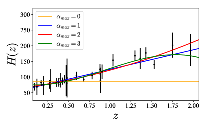
Cosmic chronometers are passively evolving old galaxies whose redshifts are known, and the expansion history of the universe can be inferred directly from their differential ages Zhang:2012mp ; Simon:2004tf ; Moresco:2012jh ; Moresco:2016mzx ; Ratsimbazafy:2017vga ; Stern:2009ep ; Moresco:2015cya . Here we will adopt the latest data as presented in (Marra:2017pst, , Table I). Figure 1 illustrates the data points as well as the fitted Hubble function obtained using the linear model formalism presented in Section V at the first, second and third order.
IV.2 Type Ia Supernovae
The second dataset that we use to reconstruct is the compressed supernova Ia Pantheon compilation (40 bins) Scolnic:2017caz .222All the data (binned and full), as well as their covariance matrices, can be downloaded from github.com/dscolnic/Pantheon. Note that, since we are performing a null test, the fact of we are using the binned catalog is not a problem in the sense of favoring the CDM model.
Type Ia Supernovas provide determinations of the distance modulus , whose theoretical prediction is related to the luminosity distance according to:
| (15) |
where the luminosity distance is given in Mpc. In the standard statistical analysis, one adds to the distance modulus the nuisance parameter , an unknown offset sum of the supernova absolute magnitude (and other possible systematics), which is degenerate with . In this analysis, as will be discussed in more details in section IV.4, the value of is related to the prior on . As we are assuming spatial flatness, the luminosity distance is related to the comoving distance via
| (16) |
where is the speed of light, so that, using (15), one obtains:
| (17) |
Finally, the normalized Hubble function can be obtained by taking the inverse of the derivative of with respect to the redshift (denoted with a prime):
| (18) |
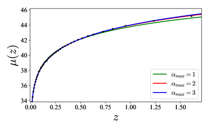
The binned Pantheon data points (subtracting ) are shown in Figure 2 together with the fitted distance modulus obtained using the linear model formalism at the first, second and third order.
IV.3 BAO
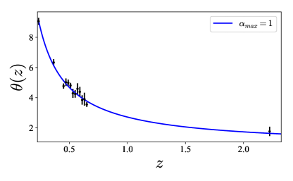
The last dataset that we use to reconstruct are model-independent angular BAO determinations obtained using the angular correlation function Sanchez:2010zg . In this case, we use 14 uncorrelated data points from Carvalho:2015ica ; Alcaniz:2016ryy ; Carvalho:2017tuu ; deCarvalho:2017xye , which are presented in Table 1 and illustrated in Figure 3 (with its first order fit). Model-independent determinations of the radial BAO scale were recently obtained in Marra:2018zzo .
| Catalog | Ref. | |||
|---|---|---|---|---|
| SDSS-DR7 | 0.235 | 9.06 | 0.23 | Alcaniz:2016ryy |
| SDSS-DR7 | 0.365 | 6.33 | 0.22 | Alcaniz:2016ryy |
| SDSS-DR10 | 0.450 | 4.77 | 0.17 | Carvalho:2015ica |
| SDSS-DR10 | 0.470 | 5.02 | 0.25 | Carvalho:2015ica |
| SDSS-DR10 | 0.490 | 4.99 | 0.21 | Carvalho:2015ica |
| SDSS-DR10 | 0.510 | 4.81 | 0.17 | Carvalho:2015ica |
| SDSS-DR10 | 0.530 | 4.29 | 0.30 | Carvalho:2015ica |
| SDSS-DR10 | 0.550 | 4.25 | 0.25 | Carvalho:2015ica |
| SDSS-DR11 | 0.570 | 4.59 | 0.36 | Carvalho:2017tuu |
| SDSS-DR11 | 0.590 | 4.39 | 0.33 | Carvalho:2017tuu |
| SDSS-DR11 | 0.610 | 3.85 | 0.31 | Carvalho:2017tuu |
| SDSS-DR11 | 0.630 | 3.90 | 0.43 | Carvalho:2017tuu |
| SDSS-DR11 | 0.650 | 3.55 | 0.16 | Carvalho:2017tuu |
| SDSS-DR12Q | 2.225 | 1.77 | 0.31 | deCarvalho:2017xye |
The theoretical BAO angular scale, in degrees, is given by,
| (19) |
where is the sound horizon of the primordial photon-baryon fluid at the drag time and is the angular diameter distance, which, in a flat universe, is related to the comoving distance by:
| (20) |
Substituting the equation above in equation (19), one obtains the following explicit relation between and ,
| (21) |
The normalized Hubble function is then obtained using equation (18).
IV.4 Further parameters
As mentioned earlier, in order to perform the null test of equation (14), it is necessary to determine also and .333When using SNe Ia data or angular BAO measurements, only is necessary as one obtains directly . We will adopt two different sets of values for these parameters. The first set is related to model-independent measurements: the local determination of obtained from low-redshift SN Ia data calibrated with loca Cepheids Riess:2018byc , and the measurement of the baryon density parameter from big bang nucleosynthesis Pettini:2012ph ,
| (22) | ||||
| (23) |
The second set of values comes from the most recent results from Planck Aghanim:2018eyx . In this work, we use the results obtained with TT,TE,EE+lowE+lensing+BAO,
| (24) | ||||
| (25) |
When using SNe Ia, we have the additional nuisance parameter . Since is fixed according to (22) or (24), we choose the respective values of from a statistical analysis of the CDM model with the Pantheon data obtained by fixing to the values previously mentioned. In order to perform the analysis, we have used the statistical code MontePython Audren:2012wb ; Brinckmann:2018cvx . When is fixed to the local determination (22), we found the best-fit value , while when is fixed to the Planck result (24) we obtained . The complete result of the statistical analysis with confidence levels is shown in Table 2 and illustrated in Figure 4.
| R18/BBN | ||||
|---|---|---|---|---|
| Planck |
When using the angular BAO determinations, one has the sound horizon as an additional parameter that must be specified. Maintaining the idea of the two sets of values we choose for the first set the model-independent result obtained from low-redshift standard rulers Verde:2016ccp Mpc. Using the local measurement of of (22), one has:
| (26) |
For the second set of values, we use the same Planck determination from Aghanim:2018eyx :
| (27) |
V Linear model formalism
Here, we will describe how to reconstruct the cosmological functions, and also their derivatives, using the Linear Model formalism (LM); see, also, Marra:2017pst ; Gomez-Valent:2018hwc ; Pinho:2018unz .
V.1 Linear Models
Let us choose a set of base functions whose linear combination will constitute the template function :
| (28) |
where is an integer. The assumption is that can describe the actual functions that we want to reconstruct: , or . Clearly, this is conditional to an appropriate choice of and the order . Usually, is a constant, often unity. The template will have coefficients.
Let us then assume that the data are given by:
| (29) |
where and are Gaussian errors with covariance matrix .
Next, we fit the template to the data and use the LM formalism to calculate the Fisher matrix relative to the parameters , which gives an exact description of the likelihood as the template is linear in its parameters. The Fisher matrix is:
| (30) |
where , and the best-fit values of are:
| (31) |
where and we defined the covariance matrix on the parameters. Summarizing, this formalism had allowed us to exactly propagate the data covariance matrix into the parameter covariance matrix .
V.2 Error on null test reconstruction
The null test is a nonlinear function of the template parameters and of the additional parameters of Section IV.4. The corresponding covariance matrix is obtained by forming an appropriate block diagonal matrix using the covariance matrices of the corresponding parameters (e.g., ). As we have chosen independent data, correlations among different datasets are not expected to be important.
In order to compute the error on due to the uncertainty encoded in the covariance matrix , a straightforward approach is to apply a change of variable from to . At the first order, the error is then given by:
| (32) |
where
| (33) |
V.3 Base functions
In order to reconstruct , and , we will adopt the following base functions, respectively:
| (34) | ||||
| (35) | ||||
| (36) |
In order to choose we will use the so-called “learning curves”, a machine learning tool.
V.4 Calibrated learning curves
The availability of large datasets is increasingly a defining feature of modern cosmology, in which data analysis has become an important component. Computations that were not possible a few decades ago can now be performed on GPU-based laptops. Machine learning includes a set of statistical techniques that allows computer systems to learn from examples, data, and experience, rather than following pre-programmed rules.
A simple method that is commonly used to choose the template order is the computation of the reduced chi-square :
| (37) |
where are the data of the full dataset with covariance matrix , and where are the best-fit parameters. If one finds that is compatible with its corresponding distribution with degrees of freedom, then the null hypothesis that is the correct model is not rejected (it is “ruled in”). While powerful in its simplicity, this method is somewhat subjective as it strongly depends on the -value threshold (e.g., ) that one is supposed to use. For example, two or more values of could be acceptable.
In order to overcome this difficultly and extract more information from the data, we will study the learning curves. These usually are used in contexts in which the data covariance matrix is not available and so a performance statistics with a known distribution (like ) cannot be built. Therefore, we will have to first generalize the standard learning curves to what we call the “calibrated learning curves.”
Let us then consider two disjoint subsets of the data set of elements: the training set and the validation set .444From now on will refer to the training set and not to the full data set. The basic idea behind the learning curves consists in using the training set to fit the model and then test the latter with the validation set. Within machine learning the fit is usually obtained by minimizing the “Mean Squared Error” (MSE):
| (38) |
where is the number of data points and , where are the parameters that minimize the MSE. From now on we will denote the minimized with just MSE. The test on the validation set is then performed by computing the “Mean Squared Prediction Error” (MSPE):
| (39) |
The use of the new data points justifies the alternative name “out-of-sample mean squared error”. Note that .
The learning curves are then the values of the MSE and the MSPE as a function of the training-set size while keep the validation-set size fixed. Usually, is 20–30% of . The expectation is that the MSE will increase as the same number of parameters will be fitted to more data, and the MSPE will decrease as the training will produce a more reliable fitted model. In particular:
-
•
an under-fitting model will feature converging but high (poor) MSE and MSPE;
-
•
an over-fitting model will feature low MSE but high MSPE because the model is fitting the noise in the training set which is different with respect to the validation set;
-
•
an optimal model will feature converging and low MSE and MSPE. Moreover, the sooner the convergence is reached, the better. Indeed, if the MSE and MSPE converge at reaching a plateau, it means that there were enough data to optimally train the model.
For more details, see, for instance hastie_09_elements-of.statistical-learning ; Abu-Mostafa ; Goodfellow-et-al-2016 ; Gron:2017:HML:3153997 .
The MSE and the MSPE do not use the data covariance matrix and, therefore, it is difficult to assess statistically their values. For example, it is not clear how to define “high”, “low” and “close to each other”. Therefore, we will calibrate the learning curve method by introducing new performance estimators that can be interpreted quantitatively in a statistical way.
A natural alternative to the MSE is the reduced chi-square function ,
| (40) |
where is the covariance matrix of the training set and is the number of fitted parameters. Assuming that is the correct model and that the data are distributed according to a multivariate Gaussian distribution of covariance matrix , it is .
A natural alternative to MSPE is,
| (41) |
where is the covariance matrix related to the validation set . As these data were not used to obtain the best-fit parameters the denominator only contains . However, the expected value of is not unity as is not the true value. Consequently, and will not converge to the same numerical value. Here, we propose a new generalization of the MSPE:
| (42) |
whose expectation value is unity as discussed in Appendix A.
In order to obtain smooth learning curves, we compute, for a fix , and for 2000 partitions, from which we then compute mean and standard deviation. Note that the performance estimators and have an expectation value of unity independently of the training set size , but this is true only if the expectation value is taken using independent training sets while here the training sets all come from the same dataset. In other words, the 2000 partitions are used to extract the average behavior of a training set of size from the full dataset .
For smaller it is quite likely to obtain low values of as its distribution is skewed towards lower values, while for larger one expects and to converge to the common value of unity. If they converge reaching a plateau it means that is the correct model and that the latter has been trained optimally by the data.
In our analysis, we adopt the following criterion in order to choose the best order : the optimal is the one for which and converge fastest to unity with a plateau. It is very important to emphasize that this learning curve procedure is completely independent of any physical assumption, depending only on data.
V.5 Learning curve results
In the following, we present the results of the learning curve analysis for the datasets of Section IV.
V.5.1 Cosmic chronometers
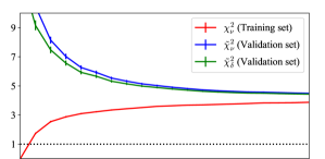
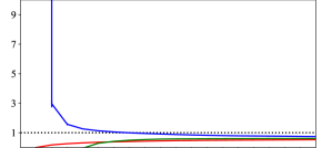
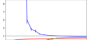
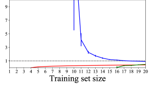
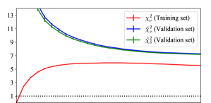
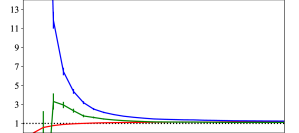
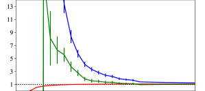
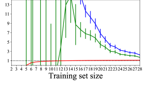
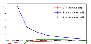
For the cosmic chronometers, we divide the 31 data points in a training set with up to 20 and a validation set with . Figure 5 shows the learning curves obtained with the template of equation (34) with (top to bottom).
The case is a clear case of under-fitting and is disfavored by the data: for the is well outside the corresponding 3 interval of (relative to the distribution with 19 degrees of freedom). This case corresponds to a constant Hubble rate, see equation (34). For the case , and converge with a plateau to a value close to 1 and within the corresponding 3 interval . According to our criteria, this is an optimal value of .
The case is similar to the case : and converge to the expected value with a plateau. Therefore, this case is also optimal, although converges to a value a little higher as compared with , signaling a minor over-fitting. It is worth pointing out that the training curves of Figure 5 feature error bars (relative to the mean) computed, as mentioned before, from 2000 partitions. Therefore, the fact that there is a gap between and is statistically significant. It is also interesting to note how the learning curves characterize the models: the case is clearly simpler than the case as less data is necessary to train it (it converges faster).
The last case shows a lack of convergence with plateau, signaling that the model is too complex to be trained by the data. Therefore, we conclude that this case is disfavored by the data. Finally, we found that and are both acceptable. If we were to use the standard analysis based on the of equation (37) for the full dataset, we would have obtained the results presented in Table 3. According to these results is also acceptable, while the learning curve analysis disfavors it.
| interval | |||
|---|---|---|---|
| 0 | 4.1 | 30 | |
| 1 | 0.57 | 29 | |
| 2 | 0.53 | 28 | |
| 3 | 0.48 | 27 |
V.5.2 Type Ia Supernovae
We divide the Pantheon sample of supernovas in a training set with up to 28 data points and a validation set with . Figure 6 shows the learning curves obtained with the template of equation (35) with (top to bottom). The case is a clear case of under-fitting and is disfavored by the data. Note that this case coincides with the first order in the cosmographic series expansion Cattoen:2007id . For the case and , and converge with a plateau to a value close to 1 and within the corresponding 3 interval . According to our criteria, these are optimal values of . Finally, shows both a lack of convergence and of plateau, signaling over-fitting.
Therefore, we found that and are both acceptable. If we were to use the standard analysis based on the of equation (37) for the full dataset, we would have obtained the results presented in Table 4. According to these results is also acceptable, while the learning curve analysis disfavors it.
V.5.3 BAO determinations
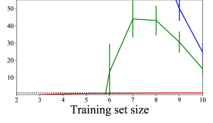
With the BAO analysis we divide the 14 data points in a training set with up to 10 data points and a validation set with . Figure 7 shows the learning curves obtained with the template of equation (36) with (top to bottom).
For the case , and converge with a plateau to a value close to 1. According to our criteria, this is the optimal value of . The case shows both a lack of convergence and of plateau, signaling over-fitting. We found, therefore, that only is acceptable. If we were to use the standard analysis based on the of equation (37) for the full dataset, we would have obtained the results presented in Table 5. According to these results is also acceptable, while the learning curve analysis disfavors it.
| interval | |||
|---|---|---|---|
| 1 | 5.3 | 38 | |
| 2 | 1.2 | 37 | |
| 3 | 1.1 | 36 | |
| 4 | 1.2 | 35 |
| interval | |||
|---|---|---|---|
| 1 | 1.0 | 12 | |
| 2 | 1.1 | 11 |
VI Gaussian Processes
A Gaussian Process (GP) is the generalization of the gaussian distribution of a random variable to the infinite function space. This mathematical approach has been successfully used as a nonparametric reconstruction method in cosmology since the pioneering works of Holsclaw2010 ; Holsclaw2011 . For instance, it has been applied to different datasets in order to calculate the dark energy equation of state Holsclaw2010 ; Holsclaw2011 ; Seikel2012 ; Zhang:2018gjb , the Hubble constant Gomez-Valent:2018hwc ; Busti:2014dua ; Licia2015 ; Li2015 , the cosmological matter perturbations Gonzalez2016 ; Gonzalez2017b ; Yin:2018mvu , and the gas deplection factor in galaxy clusters Holanda:2017cmc , among others.
A GP as a regression method is nonparametric. This means that their predictions are not restricted to a specific functional class (e.g., polinomial), but span an infinite family of classes with properties of continuity and differentiability. As this method is based on Bayesian statistics, we need to use prior and likelihood distributions to calculate the posterior distribution. Both prior and posterior distributions are defined via a mean function and a covariance matrix. The covariance quantifies the correlation between different functional values, and , at arbitrary independent variable points and .
For the prior mean function we adopt the zero function as a conservative choice (this choice is recommended to avoid biased results) and, as commonly used in the literature, we choose square exponential covariance function:
| (43) |
The so-called hyperparameters and are related with the error/variation of the reconstruction and with its smoothness, respectively. These hyperparameters can be fixed by maximizing the likelihood distribution given the observational data (for a complete description of the GP method see Seikel2012 ; Rasmussen ). To perform the GP regression, we use the python package GaPP.555Available at acgc.uct.ac.za/seikel/GAPP/index.html.
VII Results
Now, we present the reconstructions of that we obtained using the methods discussed in the previous sections. The results are divided according to the method and the data used in order to reconstruct . In all plots, for comparison purposes, we include a dotted line corresponding to the value of predicted for the CDM model according to the last results by the Planck satellite (Aghanim:2018eyx, ).
VII.1 Linear model results
Using the formalism developed in Section V, we obtain the following results:
Cosmic chronometers:
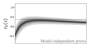
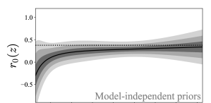
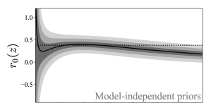
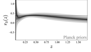
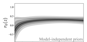
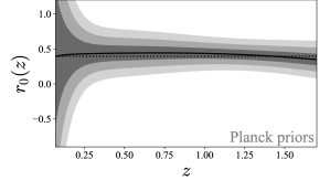
Figure 8 shows using in equation (14) the Hubble rate function reconstructed via cosmic chronometer data. For the case one detects a deviation from the standard model when the model-independent priors discussed in Section IV.4 are used. This is clearly caused by the determination of the local Hubble constant (22) which is known to be in tension with the Planck indirect determination.666See Marra:2013rba ; Camarena:2018nbr for analyses that considered the effect of cosmic variance on local . Furthermore, the test seems to suggest that there is tension only for while at higher redshift the local determination of gives a reconstruction in agreement with the value expected from Planck.
However, this interesting results loses its significance when is adopted, which was also found viable. Therefore, we conclude that better CC data are needed in order to conclude on this low-redshift tension.
Type Ia Supernovae:
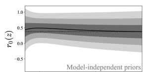
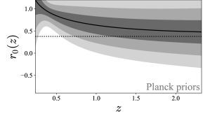
Figure 9 shows the test using the reconstruction of the distance modulus as in equations (17) and (18). We do not detect significant deviations from the Planck reference value.
BAO:
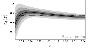
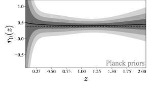
Figure 10 shows the test using the reconstruction of the BAO angular scale (19) from which is obtained via equations (21) and (18). When using Planck priors we detect a tension at with respect to the Planck reference value (but not with a higher constant reference value). This again suggests a low-redshift deviation from the standard model.
VII.2 Gaussian Process results
Using the nonparametric reconstruction of obtained via GP regression and the and priors described in Section IV.4, we calculate the null test and its confidence levels by Monte Carlo sampling.
Cosmic chronometers:
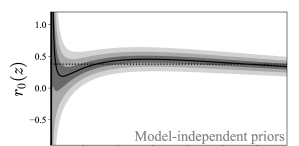
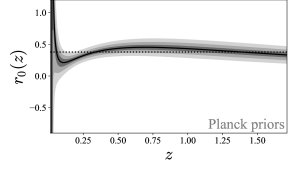
In this case, the Hubble rate is reconstructed directly from the CC data which reduces the error propagation and the probability of wiggles in the reconstruction. Figure 11 shows the calculation using GP method and Monte Carlo sampling. It is evident the similarity of these results for the two sets of priors with the results obtained using the LM formalism with (see Figure 8). This emphasizes the possibility that the tension in low- for the reconstruction via LM with may be not fundamental.
Type Ia Supernovae:
Figure 12 shows from type Ia SN data using GPs. In this case, to calculate the null test we need to transform the distance modulus data to comoving distance and then reconstruct the derivative of this quantity to obtain the Hubble rate (see Section IV.2). The determination of the derivative of propagates the error and its effect can be seen at high- where the density of the data is reduced. However, the null test is compatible with the CDM model in the entire redshift range.
BAO:
Because of the large gap in redshift between the first thirteen data points and the last one, it is not possible to find a suitable GP reconstruction compatible with a cosmological scenario without assuming a nontrivial prior mean function.
VIII Conclusions
Interacting models of CDM and DE constitute an alternative description of the dark sector which have been largely investigated. In this paper we proposed a new null test in which any deviation of the standard cosmological scenario indicates a non-minimal interaction between these two dark components. Using linear models and Gaussian processes the expansion rate is reconstructed from the latest CC, SNe Ia and BAO data. For each formalism, the same analysis was performed using two sets of values for the “external” parameters : the first set is based on model-independent results whereas the second one is obtained from the latest results of the Planck collaboration.
The test performed shows compatibility with the standard CDM model within confidence level, but some cases deserve a careful analysis. For the LM analysis using the CC data, except the case in which and the model-independent priors are used, all the other results are compatible with a constant value for . The latest Planck result is satisfied in all cases for . For only the result with Planck priors reaches satisfactory results. When the model-independent priors are used, there is a considerable tension with the latest Planck result at : in the case there is a severe tension whereas for there is a tension, which is compatible with the current tension. For all cases the error range increases when , which means that a possible interaction becoming dynamically relevant at recent times may be a viable possibility.
Still in the LM approach, all the results with SNe Ia data are compatible with a constant value and are in agreement with the latest Planck result. As for the CC result, for the result are degenerate. Lastly, for the angular BAO data, the result obtained with model-independent priors is clearly inconclusive since, for all values of , within a -range all interval is admissible for . This degenerate result is related to the big error in the model-independent determination of . However, using Planck priors, there is a disagreement signature when . For the GP analysis, all the results are consistent with a constant value and also are in agreement with the CDM Planck result.
Acknowledgements.
RvM acknowledges support from CNPq and the Federal Commission for Scholarships for Foreign Students for the Swiss Government Excellence Scholarship (ESKAS No. 2018.0443) for the academic year 2018-2019. VM thanks CNPq and FAPES for partial financial support. JEG acknowledges support from CNPq (PDJ No. 155134/2018-3). JSA acknowledges support from CNPq (Grants no. 310790/2014-0 and 400471/2014-0) and FAPERJ (Grant no. 204282).References
- (1) E. J. Copeland, M. Sami, and S. Tsujikawa, “Dynamics of dark energy,” Int.J.Mod.Phys. D15 (2006) 1753–1936, arXiv:hep-th/0603057 [hep-th].
- (2) L. Amendola and S. Tsujikawa, Dark Energy: Theory and Observations. Cambridge University Press, 2010.
- (3) M. Li, X.-D. Li, S. Wang, and Y. Wang, “Dark Energy,” Commun.Theor.Phys. 56 (2011) 525–604, arXiv:1103.5870 [astro-ph.CO].
- (4) Y. Chen, Z.-H. Zhu, J. S. Alcaniz, and Y. Gong, “Using A Phenomenological Model to Test the Coincidence Problem of Dark Energy,” Astrophys. J. 711 (2010) 439–444, arXiv:1001.1489 [astro-ph.CO].
- (5) L. Amendola, “Coupled quintessence,” Phys. Rev. D62 (2000) 043511, arXiv:astro-ph/9908023 [astro-ph].
- (6) G. Caldera-Cabral, R. Maartens, and L. A. Urena-Lopez, “Dynamics of interacting dark energy,” Phys. Rev. D79 (2009) 063518, arXiv:0812.1827 [gr-qc].
- (7) J. S. Alcaniz, H. A. Borges, S. Carneiro, J. C. Fabris, C. Pigozzo, and W. Zimdahl, “A cosmological concordance model with dynamical vacuum term,” Phys. Lett. B716 (2012) 165–170, arXiv:1201.5919 [astro-ph.CO].
- (8) R. F. vom Marttens, L. Casarini, W. S. Hipólito-Ricaldi, and W. Zimdahl, “CMB and matter power spectra with non-linear dark-sector interactions,” JCAP 1701 no. 01, (2017) 050, arXiv:1610.01665 [astro-ph.CO].
- (9) V. Marra, “Coupling dark energy to dark matter inhomogeneities,” Phys. Dark Univ. 13 (2016) 25–29, arXiv:1506.05523 [astro-ph.CO].
- (10) W. Zimdahl, “Interactions in the dark sector of the Universe,” Int. J. Geom. Meth. Mod. Phys. 11 (2014) 1460014, arXiv:1404.7334 [astro-ph.CO].
- (11) J. E. Gonzalez, H. H. B. Silva, R. Silva, and J. S. Alcaniz, “Physical constraints on interacting dark energy models,” Eur. Phys. J. C78 no. 9, (2018) 730, arXiv:1809.00439 [astro-ph.CO].
- (12) R. von Marttens, L. Casarini, D. F. Mota, and W. Zimdahl, “Cosmological constraints on parametrized interacting dark energy,” arXiv:1807.11380 [astro-ph.CO].
- (13) H. E. S. Velten, R. F. vom Marttens, and W. Zimdahl, “Aspects of the cosmological “coincidence problem”,” Eur. Phys. J. C74 no. 11, (2014) 3160, arXiv:1410.2509 [astro-ph.CO].
- (14) W. Zimdahl, W. S. Hipolito-Ricaldi, and H. E. S. Velten, “Unified models of the cosmological dark sector,” J. Phys. Conf. Ser. 314 (2011) 012057, arXiv:1012.4459 [astro-ph.CO].
- (15) W. Zimdahl, H. E. S. Velten, and W. S. Hipolito-Ricaldi, “Viscous dark fluid Universe: a unified model of the dark sector?,” Int. J. Mod. Phys. Conf. Ser. 3 (2011) 312–323, arXiv:1111.4694 [astro-ph.CO].
- (16) R. F. vom Marttens, L. Casarini, W. Zimdahl, W. S. Hipólito-Ricaldi, and D. F. Mota, “Does a generalized Chaplygin gas correctly describe the cosmological dark sector?,” Phys. Dark Univ. 15 (2017) 114–124, arXiv:1702.00651 [astro-ph.CO].
- (17) R. F. vom Marttens, W. S. Hipólito-Ricaldi, and W. Zimdahl, “Baryonic matter perturbations in decaying vacuum cosmology,” JCAP 1408 (2014) 004, arXiv:1403.0427 [astro-ph.CO].
- (18) C. Zhang, H. Zhang, S. Yuan, T.-J. Zhang, and Y.-C. Sun, “Four new observational data from luminous red galaxies in the Sloan Digital Sky Survey data release seven,” Res. Astron. Astrophys. 14 no. 10, (2014) 1221–1233, arXiv:1207.4541 [astro-ph.CO].
- (19) J. Simon, L. Verde, and R. Jimenez, “Constraints on the redshift dependence of the dark energy potential,” Phys. Rev. D71 (2005) 123001, arXiv:astro-ph/0412269 [astro-ph].
- (20) M. Moresco et al., “Improved constraints on the expansion rate of the Universe up to z 1.1 from the spectroscopic evolution of cosmic chronometers,” JCAP 1208 (2012) 006, arXiv:1201.3609 [astro-ph.CO].
- (21) M. Moresco, L. Pozzetti, A. Cimatti, R. Jimenez, C. Maraston, L. Verde, D. Thomas, A. Citro, R. Tojeiro, and D. Wilkinson, “A 6% measurement of the Hubble parameter at : direct evidence of the epoch of cosmic re-acceleration,” JCAP 1605 no. 05, (2016) 014, arXiv:1601.01701 [astro-ph.CO].
- (22) A. L. Ratsimbazafy, S. I. Loubser, S. M. Crawford, C. M. Cress, B. A. Bassett, R. C. Nichol, and P. Väisänen, “Age-dating Luminous Red Galaxies observed with the Southern African Large Telescope,” Mon. Not. Roy. Astron. Soc. 467 no. 3, (2017) 3239–3254, arXiv:1702.00418 [astro-ph.CO].
- (23) D. Stern, R. Jimenez, L. Verde, M. Kamionkowski, and S. A. Stanford, “Cosmic Chronometers: Constraining the Equation of State of Dark Energy. I: H(z) Measurements,” JCAP 1002 (2010) 008, arXiv:0907.3149 [astro-ph.CO].
- (24) M. Moresco, “Raising the bar: new constraints on the Hubble parameter with cosmic chronometers at z 2,” Mon. Not. Roy. Astron. Soc. 450 no. 1, (2015) L16–L20, arXiv:1503.01116 [astro-ph.CO].
- (25) V. Marra and D. Sapone, “Null tests of the standard model using the linear model formalism,” Phys. Rev. D97 no. 8, (2018) 083510, arXiv:1712.09676 [astro-ph.CO].
- (26) D. M. Scolnic et al., “The Complete Light-curve Sample of Spectroscopically Confirmed Type Ia Supernovae from Pan-STARRS1 and Cosmological Constraints from The Combined Pantheon Sample,” arXiv:1710.00845 [astro-ph.CO].
- (27) E. Sanchez, A. Carnero, J. Garcia-Bellido, E. Gaztanaga, F. de Simoni, M. Crocce, A. Cabre, P. Fosalba, and D. Alonso, “Tracing The Sound Horizon Scale With Photometric Redshift Surveys,” Mon. Not. Roy. Astron. Soc. 411 (2011) 277–288, arXiv:1006.3226 [astro-ph.CO].
- (28) G. C. Carvalho, A. Bernui, M. Benetti, J. C. Carvalho, and J. S. Alcaniz, “Baryon Acoustic Oscillations from the SDSS DR10 galaxies angular correlation function,” Phys. Rev. D93 no. 2, (2016) 023530, arXiv:1507.08972 [astro-ph.CO].
- (29) J. S. Alcaniz, G. C. Carvalho, A. Bernui, J. C. Carvalho, and M. Benetti, “Measuring baryon acoustic oscillations with angular two-point correlation function,” Fundam. Theor. Phys. 187 (2017) 11–19, arXiv:1611.08458 [astro-ph.CO].
- (30) G. C. Carvalho, A. Bernui, M. Benetti, J. C. Carvalho, and J. S. Alcaniz, “Measuring the transverse baryonic acoustic scale from the SDSS DR11 galaxies,” arXiv:1709.00271 [astro-ph.CO].
- (31) E. de Carvalho, A. Bernui, G. C. Carvalho, C. P. Novaes, and H. S. Xavier, “Angular Baryon Acoustic Oscillation measure at from the SDSS quasar survey,” JCAP 1804 no. 04, (2018) 064, arXiv:1709.00113 [astro-ph.CO].
- (32) V. Marra and E. G. C. Isidro, “Model-independent radial BAO constraints from SDSS-III DR12,” arXiv:1808.10695 [astro-ph.CO].
- (33) A. G. Riess et al., “Milky Way Cepheid Standards for Measuring Cosmic Distances and Application to Gaia DR2: Implications for the Hubble Constant,” Astrophys. J. 861 no. 2, (2018) 126, arXiv:1804.10655 [astro-ph.CO].
- (34) M. Pettini and R. Cooke, “A new, precise measurement of the primordial abundance of Deuterium,” Mon. Not. Roy. Astron. Soc. 425 (2012) 2477–2486, arXiv:1205.3785 [astro-ph.CO].
- (35) Planck Collaboration, N. Aghanim et al., “Planck 2018 results. VI. Cosmological parameters,” arXiv:1807.06209 [astro-ph.CO].
- (36) B. Audren, J. Lesgourgues, K. Benabed, and S. Prunet, “Conservative Constraints on Early Cosmology: an illustration of the Monte Python cosmological parameter inference code,” JCAP 1302 (2013) 001, arXiv:1210.7183 [astro-ph.CO].
- (37) T. Brinckmann and J. Lesgourgues, “MontePython 3: boosted MCMC sampler and other features,” arXiv:1804.07261 [astro-ph.CO].
- (38) L. Verde, J. L. Bernal, A. F. Heavens, and R. Jimenez, “The length of the low-redshift standard ruler,” Mon. Not. Roy. Astron. Soc. 467 no. 1, (2017) 731–736, arXiv:1607.05297 [astro-ph.CO].
- (39) A. Gómez-Valent and L. Amendola, “ from cosmic chronometers and Type Ia supernovae, with Gaussian Processes and the novel Weighted Polynomial Regression method,” JCAP 1804 no. 04, (2018) 051, arXiv:1802.01505 [astro-ph.CO].
- (40) A. M. Pinho, S. Casas, and L. Amendola, “Model-independent reconstruction of the linear anisotropic stress ,” arXiv:1805.00027 [astro-ph.CO].
- (41) T. Hastie, R. Tibshirani, and J. Friedman, The elements of statistical learning: data mining, inference and prediction. Springer, 2 ed., 2009. http://www-stat.stanford.edu/~tibs/ElemStatLearn/.
- (42) Y. S. Abu-Mostafa, M. Magdon-Ismail, and H.-T. Lin, Learning From Data. AMLBook, 2012.
- (43) I. Goodfellow, Y. Bengio, and A. Courville, Deep Learning. MIT Press, 2016. http://www.deeplearningbook.org.
- (44) A. Gron, Hands-On Machine Learning with Scikit-Learn and TensorFlow: Concepts, Tools, and Techniques to Build Intelligent Systems. O’Reilly Media, Inc., 1st ed., 2017.
- (45) C. Cattoen and M. Visser, “Cosmography: Extracting the Hubble series from the supernova data,” arXiv:gr-qc/0703122 [gr-qc].
- (46) T. Holsclaw, U. Alam, B. Sanso, H. Lee, K. Heitmann, S. Habib, and D. Higdon, “Nonparametric Dark Energy Reconstruction from Supernova Data,” Phys. Rev. Lett. 105 (2010) 241302, arXiv:1011.3079 [astro-ph.CO].
- (47) T. Holsclaw, U. Alam, B. Sanso, H. Lee, K. Heitmann, S. Habib, and D. Higdon, “Nonparametric Reconstruction of the Dark Energy Equation of State from Diverse Data Sets,” Phys. Rev. D84 (2011) 083501, arXiv:1104.2041 [astro-ph.CO].
- (48) M. Seikel, C. Clarkson, and M. Smith, “Reconstruction of dark energy and expansion dynamics using Gaussian processes,” JCAP 1206 (2012) 036, arXiv:1204.2832 [astro-ph.CO].
- (49) M.-J. Zhang and H. Li, “Gaussian processes reconstruction of dark energy from observational data,” Eur. Phys. J. C78 no. 6, (2018) 460, arXiv:1806.02981 [astro-ph.CO].
- (50) V. C. Busti, C. Clarkson, and M. Seikel, “Evidence for a Lower Value for from Cosmic Chronometers Data?,” Mon. Not. Roy. Astron. Soc. 441 (2014) 11, arXiv:1402.5429 [astro-ph.CO].
- (51) L. Verde, P. Protopapas, and R. Jimenez, “The expansion rate of the intermediate universe in light of Planck,” Physics of the Dark Universe 5 (Dec., 2014) 307–314, arXiv:1403.2181 [astro-ph.CO].
- (52) Z. Li, J. E. Gonzalez, H. Yu, Z.-H. Zhu, and J. S. Alcaniz, “Constructing a cosmological model-independent Hubble diagram of type Ia supernovae with cosmic chronometers,” Phys. Rev. D93 no. 4, (2016) 043014, arXiv:1504.03269 [astro-ph.CO].
- (53) J. E. Gonzalez, J. S. Alcaniz, and J. C. Carvalho, “Non-parametric reconstruction of cosmological matter perturbations,” JCAP 1604 no. 04, (2016) 016, arXiv:1602.01015 [astro-ph.CO].
- (54) J. E. Gonzalez, “Reconstruction of cosmological matter perturbations in Modified Gravity,” Phys. Rev. D96 no. 12, (2017) 123501, arXiv:1710.07656 [astro-ph.CO].
- (55) Z.-Y. Yin and H. Wei, “Non-parametric Reconstruction of Growth Index via Gaussian Processes,” arXiv:1808.00377 [astro-ph.CO].
- (56) R. F. L. Holanda, V. C. Busti, J. E. Gonzalez, F. Andrade-Santos, and J. S. Alcaniz, “Cosmological constraints on the gas depletion factor in galaxy clusters,” JCAP 1712 no. 12, (2017) 016, arXiv:1706.07321 [astro-ph.CO].
- (57) C. Rasmussen and C. Williams, Gaussian Processes for Machine Learning. MIT Press, 2006.
- (58) V. Marra, L. Amendola, I. Sawicki, and W. Valkenburg, “Cosmic variance and the measurement of the local Hubble parameter,” Phys. Rev. Lett. 110 no. 24, (2013) 241305, arXiv:1303.3121 [astro-ph.CO].
- (59) D. Camarena and V. Marra, “Impact of the cosmic variance on on cosmological analyses,” Phys. Rev. D98 no. 2, (2018) 023537, arXiv:1805.09900 [astro-ph.CO].
Appendix A Calibrated MSPE
In order to obtain a performance estimator with the same expectation value of , let us rewrite equation (41) as:
| (44) | ||||
where is the true value of computed in , and in the second line we have omitted cross-product terms whose expectation value is zero because of the independence between the data used to fit the model and the data.777Note that, if and are partitions of a correlated dataset, one is neglecting the correlation between these two partitions. The expectation value of the first term is clearly . The expectation value of the second term is not trivial:
| (45) | ||||
In the following we will use the notation that is a random variable when inside expectation values while it is when outside, that is, we use the best-fit model in order to estimate the true model .
The first term in the last equation is the variance of which can be computed, as in Section V.2, through a change of variables using the covariance matrix on the parameters obtained from equation (30) using the training set:
| (46) | ||||
where we have used equation (28). Note that, thanks to the linearity in the parameters, the best fits were not used and this computation is exact rather than only valid at the first order in a Taylor expansion.
The second term is,
| (47) |
Using again equation (28) one finds:
| (48) | ||||
where we used the best-fit parameters in order to estimate the true values of the parameters. Combining the equations (45), (46) and (48), the equation (44) can be rewritten as:
| (49) |
where:
It is then straightforward to obtain that:
| (50) |
where is the covariance matrix on the parameters obtained from equation (30) using the validation set, that was not used to fit the model.
Motivated by this results, we propose a new generalization of the MSPE:
| (51) |
whose expectation value is unity. From the previous equation it follows that for large sets the correction should be negligible. Indeed, as training and validation sets have usually sizes of the same order of magnitude, one has .
Appendix B learning_curve package
All the learning curves presented in this work were obtained using the package learning_curve. The package learning_curve consists of three python scripts to compute and plot learning curves. The three python scripts are the following:
-
•
learning_curve.py: general parallelized script for computing learning curves for any linear template function.
-
•
learning_curve_linear.py: script for computing and plotting learning curves for some specific template functions (polynomial, log, inverse or square).
-
•
plot.py: script for plotting the learning curves from the output files obtained using the script learning_curve.py.
In this work, only the learning_curve_linear.py script was used, because its template functions coincide with the template functions adopted in the present analysis. The package is available for download at github.com/rodrigovonmarttens/learning_curve.