Phase transition for the once-excited random walk on general trees

Abstract.

The phase transition of $M$-digging random on a general tree was studied by Collevecchio, Huynh and Kious [4]. In this paper, we study particularly the critical $M$-digging random walk on a superperiodic tree that is proved to be recurrent.
We keep using the techniques introduced by Collevecchio, Kious and Sidoravicius [5] with the aim of investigating the phase transition of Once-excited random walk on general trees.
In addition, we prove if $\mathcal{T}$ is a tree whose branching number is larger than $1$, any multi-excited random walk on $\mathcal{T}$ moving, after excitation, like a simple random walk is transient.

1. Introduction

In this paper, we study a particular case of multi-excited random walks on trees, introduced by Volkov [11], called the once-excited random walk.
Let $M\in\mathbb{N}$, $(\lambda_{1},...,\lambda_{M})\in(\mathbb{R}_{+})^{M}$ and $\lambda>0$. Let $\mathcal{T}$ be an infinite, locally-finite, tree rooted at $\varrho$. The $(\lambda_{1},...,\lambda_{M},\lambda)$-ERW on $\mathcal{T}$, is a nearest-neighbor random walk $(X_{n})$ started at $\varrho$ such that if $X_{n}$ is on a site for the $i$-th time for $i\leq M$, then the walker takes a random step of a biased random walk with bias $\lambda_{i}$ (i.e. it jumps on its parent with probability proportional to $1$, or jumps on a particular offspring of $\nu$ with probability proportional to $\lambda_{i}$); and if $i>M$, then $X_{n}$ takes a random step of a biased random walk with bias $\lambda$. In the case $M=1$, it is called the once-excited random walk with parameters $(\lambda_{1},\lambda)$. We write $(\lambda_{1},\lambda)$-OERW for $(\lambda_{1},\lambda)$-ERW. The definition of the model and the vocabulary will be made clear in Section 2.3.

Unlike the case of once-reinforced random walk in [5] or digging-random walk in [4], the phase transition of OERW does not depend only on the branching-ruin number and the branching number of tree (see Section 4 for more details). In the case $\mathcal{T}$ is a spherically symmetric tree, we give a sharp phase transition recurrence/transience in terms of their branching number and branching-ruin number and others.

In the following, we denote $br(\mathcal{T})$ the branching number of a tree $\mathcal{T}$ and $br_{r}(\mathcal{T})$ the branching-ruin number of a tree $\mathcal{T}$, see (2.1) and (2.2) for their definitions. Let us simply emphasize that, for any tree $\mathcal{T}$, its branching number is at least one, i.e. $br(\mathcal{T})\geq 1$, whereas the branching-ruin number is nonnegative, i.e. $br_{r}(\mathcal{T})\geq 0$.

A tree $\mathcal{T}$ is said to be spherically symmetric if for every vertex $\nu$, $\deg\nu$ depends only on $\left|\nu\right|$, where $\left|\nu\right|$ denote its distance from the root and $\deg\nu$ is its number of neighbors. Let $\mathcal{T}$ be a spherically symmetric tree. For any $n\geq 0$, let $x_{n}$ be the number of children of a vertex at level $n$. For any $\lambda_{1}\geq 0$ and $\lambda>0$, we define the following quantities:

(1.1) $$\alpha(\mathcal{T},\lambda_{1},\lambda)=\liminf_{n\rightarrow\infty}\left(\prod_{i=1}^{n}\frac{\lambda^{2}+(x_{i}-1)\lambda_{1}\lambda+\lambda_{1}}{1+x_{i}\lambda_{1}}\right)^{1/n}.$$

(1.2) $$\beta(\mathcal{T},\lambda_{1},\lambda)=\limsup_{n\rightarrow\infty}\left(\prod_{i=1}^{n}\frac{\lambda^{2}+(x_{i}-1)\lambda_{1}\lambda+\lambda_{1}}{1+x_{i}\lambda_{1}}\right)^{1/n}.$$

(1.3) $$\gamma(\mathcal{T},\lambda_{1})=\liminf_{n\rightarrow\infty}\frac{-\sum_{i=1}^{n}\ln\left[1-\frac{(x_{i}-1)\lambda_{1}+2}{(1+x_{i}\lambda_{1})i}\right]}{\ln n}.$$

(1.4) $$\eta(\mathcal{T},\lambda_{1})=\limsup_{n\rightarrow\infty}\frac{-\sum_{i=1}^{n}\ln\left[1-\frac{(x_{i}-1)\lambda_{1}+2}{(1+x_{i}\lambda_{1})i}\right]}{\ln n}.$$

Theorem 1.

Let $\mathcal{T}$ be a spherically symmetric tree, and let $\lambda_{1}\geq 0$, $\lambda>0$. Denote ${\bf X}$ the $(\lambda_{1},\lambda)$-OERW on $\mathcal{T}$. Assume that there exists a constant $M>0$ such that $\sup_{\nu\in V}\deg\nu\leq M$, then we have

1. in the case $\lambda=1$, if $\eta(\mathcal{T},\lambda_{1})<br_{r}(\mathcal{T})$ then ${\bf X}$ is transient and if $\gamma(\mathcal{T},\lambda_{1})>br_{r}(\mathcal{T})$ then ${\bf X}$ is recurrent;

2. assume that $\lambda_{1}\geq 0$, $\lambda\neq 1$ and $br(\mathcal{T})>1$, if $\beta(\mathcal{T},\lambda_{1},\lambda)<\frac{1}{br(\mathcal{T})}$ then ${\bf X}$ is recurrent and if $\alpha(\mathcal{T},\lambda_{1},\lambda)>\frac{1}{br(\mathcal{T})}$ then ${\bf X}$ is transient.

Note that, for a $b$-ary tree, we have $br(\mathcal{T})=b$ and

(1.5) $$\alpha(\mathcal{T},\lambda_{1},\lambda)=\beta(\mathcal{T},\lambda_{1},\lambda)=\frac{\lambda^{2}+(b-1)\lambda\lambda_{1}+\lambda_{1}}{1+b\lambda_{1}}$$

and our result therefore agrees with Corollary 1.6 of [1]. In [1], the authors prove that the walk is recurrent at criticality on regular trees, but this is not expected to be true on any tree). For instance, if $\lambda_{1}=\lambda$, the $(\lambda,\lambda)$-OERW $\bf X$ is the biased random walk with parameter $\lambda$. Therefore $\bf X$ may be recurrent or transient at criticality (see [2], proposition 22).

Volkov [11] conjectured that, any cookie random walk which moves, after excitation, like a simple random walk (i.e. $\lambda=1$) is transient on any tree containing the binary tree. This conjecture was proved by Basdevant and Singh [1]. Here, we extend this conjecture to any tree $\mathcal{T}$ whose branching number is larger than $1$:

Theorem 2.

Let $(\lambda_{1},...,\lambda_{M})\in(\mathbb{R}_{+})^{M}$ and consider $(\lambda_{1},...,\lambda_{M},1)$-ERW $\bf X$ on an infinite, locally finite, rooted tree $\mathcal{T}$. If $br(\mathcal{T})>1$, then $\bf X$ is transient.

The techniques used our paper rely on the strategy adopted in [5] or [4]. In particular, for the proof of transience, we here too view the set of edges crossed by ${\bf X}$ before returning to $\varrho$ as the cluster of the root in a particular correlated percolation.
There are two key ingredients that allow us to use the rest of the strategy from [5]. First, we need to define extensions of ${\bf X}$, which are a family of coupled continuous-time versions of ${\bf X}$ defined on subtrees of $\mathcal{T}$. As in [5], we do this through Rubin’s construction in Section 7. But we will see in Section 7, this construction is actually very different to a once-reinforced random walk in [5] or $M$-digging random walk in [4].
Second, we need to prove that the correlated percolation mentioned above is in fact a quasi-independent percolation, see Lemma 17. From there, the problem boils down to proving that a certain quasi-independent percolation is supercritical.
We refer to Theorem 4 for the more general result on a general tree.

2. The model

First, we review some basic definitions of graph theory and then we define the model of multi-excited random walk on trees which was introduced by Volkov[11] and then made general by Basdevant and Singh[1].

2.1. Notation

Let $\mathcal{T}=(V,E)$ be an infinite, locally finite, rooted tree with the root $\varrho$.
Given two vertices $\nu,\mu$ of $\mathcal{T}$, we say that $\nu$ and $\mu$ are neighbors, denoted $\nu\sim\mu$, if $\{\nu,\mu\}$ is an edge of $\mathcal{T}$.
Let $\nu,\mu\in V\setminus\{\varrho\}$, the distance between $\nu$ and $\mu$, denoted by $d(\nu,\mu)$, is the minimum number of edges of the unique self-avoiding paths joining $x$ and $y$. The distance between $\nu$ and $\varrho$ is called height of $\nu$, denoted by $|\nu|$. The parent of $\nu$ is the vertex $\nu^{-1}$ such that $\nu^{-1}\sim\nu$ and $|\nu^{-1}|=|\nu|-1$. We also call $\nu$ is a child of $\nu^{-1}$.
For any $\nu\in V$, denote by $\partial(\nu)$ the number of children of $\nu$ and $\{\nu_{1},...,\nu_{\partial\nu}\}$ is the set of children of $\nu$. We define an order on $\mathcal{T}$ by the following way. For all $\nu$ and $\mu$, we say that $\nu\leq\mu$ if the unique self-avoiding path joining $\varrho$ and $\mu$ contains $\nu$, and we say that $\nu<\mu$ if moreover $\nu\neq\mu$.
Denote by $\mathcal{T}_{n}$ the set of vertices of $\mathcal{T}$ at height $n$. For any $\nu\in\mathcal{T}$, denote by $\mathcal{T}^{\nu}$ the biggest sub-tree of $\mathcal{T}$ rooted at $\nu$, i.e. $\mathcal{T}^{u}=\mathcal{T}[V^{u}]$, where

$$V^{u}:=\left\{v\in V(T):u\leq v\right\}.$$

For any edge $e$ of $\mathcal{T}$, denote by $e^{+}$ and $e^{-}$ its endpoints with $|e^{+}|=|e^{-}|+1$, and we define the height of $e$ as $|e|=|e^{+}|$.
For two edges $e$ and $g$ of $\mathcal{T}$, we write $g\leq e$ if $g^{+}\leq e^{+}$ and $g<e$ if moreover $g^{+}\neq e^{+}$. For two vertices $\nu$ and $\mu$ of $\mathcal{T}$ such that $\nu<\mu$, we denote by $[\nu,\mu]$ the unique self-avoiding path joining $\nu$ to $\mu$. For two neighboring vertices $\nu$ and $\mu$, we use the slight abuse of notation $[\nu,\mu]$ to denote the edge with endpoints $\nu$ and $\mu$ (note that we allow $\mu<\nu$).
For two edges $e_{1}$ and $e_{2}$ of $E$, denote by $e_{1}\wedge e_{2}$ the vertex with maximal distance from the root such that $e_{1}\wedge e_{2}\leq e_{1}^{+}$ and $e_{1}\wedge e_{2}\leq e_{2}^{+}$.

Finally, we define a particular class of trees, which is called superperiodic tree. Let $\mathcal{T}_{1}=(V_{1},E_{1})$ and $\mathcal{T}_{2}=(V_{2},E_{2})$ be two trees. A morphism of $\mathcal{T}_{1}$ to $\mathcal{T}_{2}$ is a map $f:\mathcal{T}_{1}\rightarrow\mathcal{T}_{2}$ such that whenever $\nu$ and $\mu$ and $\mu$ are incident in $\mathcal{T}_{1}$, then so are $f(\nu)$ and $f(\mu)$ in $\mathcal{T}_{2}$.
Let $N\geq 0$. An infinite, locally finite and rooted tree $\mathcal{T}$ with the root $\varrho$, is said to be $N$-superperiodic if for every $\nu\in V(\mathcal{T})$, there exists an injective morphism $f:\mathcal{T}\rightarrow\mathcal{T}^{f(o)}$ with $f(o)\in\mathcal{T}^{\nu}$ and $|f(o)|-|\nu|\leq N$. A tree $\mathcal{T}$ is called superperiodic tree if there exists $N\geq 0$ such that it is $N$-superperiodic.

2.2. Some quantities on trees

In this section, we review the definitions of branching number, growth rate and branching-ruin number. We refer the reader to ([6] , [8]) for more details on the branching number and growth rate and [5] for more details on the branching-ruin number.

In order to define the branching number and the branching-ruin number of a tree, we will need the notion of cutsets.
Let $\mathcal{T}$ be an infinite, locally finite and rooted tree. A cutset in $\mathcal{T}$ is a set $\pi$ of edges such that every infinite simple path from $a$ must include an edge in $\pi$. The set of cutsets is denoted by $\Pi$.

The branching number of $\mathcal{T}$ is defined as

(2.1) $$br(\mathcal{T})=\sup\left\{\gamma>0:\inf_{\pi\in\Pi}\ \sum_{e\in\pi}\gamma^{-\left|e\right|}>0\right\}\in[1,\infty].$$

The branching-ruin number of $\mathcal{T}$ is defined as

(2.2) $$br_{r}(\mathcal{T})=\sup\left\{\gamma>0:\inf_{\pi\in\Pi}\ \sum_{e\in\pi}|e|^{-\gamma}>0\right\}\in[0,\infty].$$

These quantities depend on the structure of the tree. If $\mathcal{T}$ is spherically symmetric, then there is really no information in the tree than that contained in the sequence $\left(|\mathcal{T}_{n}|,n\geq 0\right)$. Therefore, a tree which is spherically symmetric and whose $n$ generation grows like $b^{n}$ (resp. $n^{b}$), for $b\geq 1$, has a branching number (resp. branching-ruin number) equal to $b$. For more general trees, this becomes more complicated. In the other word, there exists a tree whose $n$ generation grows like $b^{n}$ (resp. $n^{b}$), for $b\geq 1$, but its branching number (resp. branching-ruin number) is not equal to $b$. For instance, the tree 1-3 in ([8], page 4) is an example.

Finally, we review the definition of growth rate of an infinite, locally finite and rooted tree $\mathcal{T}$. Define the lower growth rate of $\mathcal{T}$ by

(2.3) $$\underline{gr(\mathcal{T})}=\liminf\left|\mathcal{T}_{n}\right|^{\frac{1}{n}}.$$

Similarly, we can define upper growth rate of $\mathcal{T}$ by

(2.4) $$\overline{gr(\mathcal{T})}=\limsup\left|\mathcal{T}_{n}\right|^{\frac{1}{n}}.$$

In the case $\overline{gr(\mathcal{T})}=\underline{gr(\mathcal{T})}$, we define the growth rate of $\mathcal{T}$, denoted by $gr(\mathcal{T})$, by taking the common value of $\overline{gr(\mathcal{T})}$ and $\underline{gr(\mathcal{T})}.$

Now, we state a relationship between the branching number and growth rate of a superperiodic tree.

Theorem 3 (see [8]).

Let $\mathcal{T}$ be a $N$-superperiodic tree with $\overline{gr}(\mathcal{T})<\infty$. Then the growth rate of $\mathcal{T}$ ​​exists and $gr(\mathcal{T})=br(\mathcal{T})$. Moreover, we have $|\mathcal{T}_{n}|\leq gr(\mathcal{T})^{n+N}$.

2.3. Definition of the model

Now, we define the model of multi-excited random walk on trees. Let $\mathcal{C}=(\lambda_{1},...,\lambda_{M};\lambda)\in\left(\mathbb{R}_{+}\right)^{M}\times\mathbb{R}_{+}^{*}$ and $\mathcal{T}=(V,E)$ be an infinite, locally finite and rooted tree with the root $\varrho$. A $\mathcal{C}$ multi-excited random walk is a stochastic process $\bf X$ $:=(X_{n})_{n\geq 0}$ defined on some probability space, taking the values in $\mathcal{T}$ with the transition probability defined by:

$$\mathbb{P}(X_{0}=\varrho)=1,$$

$$\mathbb{P}\left(X_{n+1}=(X_{n})_{i}|X_{0},\cdots,X_{n}\right)=\left\{\begin{matrix}\frac{\lambda_{j}}{1+\partial(X_{n})\lambda_{j}}\,\,\,\,\text{ if }j\leq M\\ \frac{\lambda}{1+\partial(X_{n})\lambda}\,\,\,\,\text{ if }j>M\end{matrix}\right.$$

$$\mathbb{P}\left(X_{n+1}=X_{n}^{-1}|X_{0},\cdots,X_{n}\right)=\left\{\begin{matrix}\frac{1}{1+\partial(X_{n})\lambda_{j}}\,\,\,\,\text{ if }j\leq M\\ \frac{1}{1+\partial(X_{n})\lambda}\,\,\,\,\text{ if }j>M\end{matrix}\right.$$

where $i\in\{1,\cdots,k\}$ and $j=|\{0\leq k\leq n:X_{k}=X_{n}\}|$.

We have some particular cases:

• If $\mathcal{C}=(0,...,0;\lambda)$, then $\mathcal{C}$ multi-excited random walk is $M$-digging random walk with parameter $\lambda$ ($M$-DRW_λ), which was studied in [4].

• If $M=0$, then $\mathcal{C}$ multi-excited random walk is the biased random walk with parameter $\lambda$, which was studied in [7].

• If $\mathcal{C}=(\lambda_{1};\lambda)$, then $\mathcal{C}$ multi-excited random walk is $(\lambda_{1},\lambda)$-OERW.

The return time of $\bf X$ to a vertex $\nu$ is defined by:

(2.5) $$T(\nu):=\inf\{n\geq 1:X_{n}=\nu\}.$$

We say that $\bf X$ is transient if

(2.6) $$\mathbb{P}\left(T(\varrho)=\infty\right)>0.$$

Otherwise, we say that $\bf X$ is recurrent.

3. Main results

3.1. Main results about Once-excited random walk

Let $\lambda_{1}\geq 0$ and $\lambda>0$ and we consider the model $(\lambda_{1},\lambda)$-OERW on an infinite, locally finite and rooted tree $\mathcal{T}$. First, we define the following functions. For any $e\in E$, we set $\psi(e,\lambda)=1$ and $\phi(e,\lambda_{1},\lambda)=1$ if $|e|=1$ and, for any $e\in E$ with $|e|>1$, we set

(3.1) $$\begin{split}\psi(e,\lambda)&=\frac{\lambda^{|e|-1}-1}{\lambda^{|e|}-1}\text{ if }\lambda\neq 1,\\ \psi(e,\lambda)&=\frac{|e|-1}{|e|}\text{ if }\lambda=1.\\ \end{split}$$

(3.2) $$\phi(e,\lambda_{1},\lambda)=\frac{\lambda_{1}}{1+\partial(e^{-})\lambda_{1}}+\frac{1}{1+\partial(e^{-})\lambda_{1}}\psi(e,\lambda)\psi(e^{-1},\lambda)+\frac{(\partial(e^{-})-1)\lambda_{1}}{1+\partial(e^{-})\lambda_{1}}\psi(e,\lambda)$$

Finally, for any $e\in E$, we define:

(3.3) $$\Psi(e,\lambda_{1},\lambda)=\prod_{g\leq e}\phi(g,\lambda_{1},\lambda).$$

We refer the reader to Lemma 14 for the probabilistic interpretation of these functions.

In the following, we assume that

(3.4) $$\exists M\in\mathbb{N}\text{ such that }\sup\{\deg\nu:\nu\in V\}\leq M.$$

Let us define the quantity $RT(\mathcal{T},{\bf X})$ which was introduced in [5]:

(3.5) $$RT(\mathcal{T},{\bf X})=\sup\{\gamma>0:\inf_{\pi\in\Pi}\sum_{e\in\pi}\left(\Psi(e)\right)^{\gamma}>0\}.$$

Theorem 4.

Consider an $(\lambda_{1},\lambda)$-OERW on an infinite, locally finite, rooted tree $\mathcal{T}$, with parameters $\lambda_{1}\geq 0$ and $\lambda>0$. If $RT(\mathcal{T},{\bf X})<1$ then ${\bf X}$ is recurrent. If $RT(\mathcal{T},{\bf X})>1$ and if (3.4) holds, then ${\bf X}$ is transient.

In the following, we consider the case $\mathcal{T}$ is spherically symmetric.

Lemma 5.

Consider a $(\lambda_{1},\lambda)$-OERW ${\bf X}$ on a spherically symmetric $\mathcal{T}$, with parameters $\lambda_{1}\geq 0$ and $\lambda>0$. Assume that there exists a constant $M>0$ such that $\sup_{\nu\in V}\deg\nu\leq M$. We have that

1. in the case $\lambda=1$, if $\eta(\mathcal{T},\lambda_{1})<br_{r}(\mathcal{T})$ then $RT(\mathcal{T},{\bf X})>1$ and if $\gamma(\mathcal{T},\lambda_{1})>br_{r}(\mathcal{T})$ then $RT(\mathcal{T},{\bf X})<1$;

2. assume that $\lambda_{1}\geq 0$, $\lambda\neq 1$ and $br(\mathcal{T})>1$, if $\beta(\mathcal{T},\lambda_{1},\lambda)<\frac{1}{br(\mathcal{T})}$ then $RT(\mathcal{T},{\bf X})<1$ and if $\alpha(\mathcal{T},\lambda_{1},\lambda)>\frac{1}{br(\mathcal{T})}$ then $RT(\mathcal{T},{\bf X})>1$.

Note that Theorem 1 is a consequence of Theorem 4 and Lemma 5.

3.2. Main results about critical $M$-Digging random walk

Let $M\in\mathbb{N}^{*}$, $\lambda>0$ and we consider the model $M$-DRW_λ on an infinite, locally finite and rooted tree $\mathcal{T}$. In [4], Collevecchio-Huynh-Kious was proved that there is a phase transition with respect to the parameter $\lambda$, i.e there exists a critical parameter $\lambda_{c}$. A natural question that arises: what happens if $\lambda=\lambda_{c}$? As we said in the introduction, there is no a good answer for this question.

In [1], Basdevant-Singh proved the critical $M$-digging random walk is recurrent on the regular trees. In this paper, we prove the critical $M$-digging random walk is still recurrent on a particular class of trees which contains the regular trees.

Theorem 6.

Let $M\in\mathbb{N}^{*}$ and $\mathcal{T}$ be a superperiodic tree whose upper-growth rate is finite. Then the critical $M$-digging random walk on $\mathcal{T}$ is recurrent.

4. An example

In this section, we give an example to prove that the phase transition of once-excited random walk $(\lambda_{1},\lambda)-OERW$ on a tree $\mathcal{T}$ does not depend only on the branching-ruin number and the branching number of $\mathcal{T}$.

If $\mathcal{T}$ is a spherically symmetric tree, recall that $x_{n}(\mathcal{T})$ is the number of children of a vertex at level $n$.

Let $\mathcal{T}$ (resp. $\mathcal{\widetilde{T}}$) be a spherically symmetric such that for any $n\geq 0$, we have $x_{n}(\mathcal{T})=2$ (resp. $x_{n}(\mathcal{\widetilde{T}})=1$ if $n$ is odd and $x_{n}(\mathcal{\widetilde{T}})=4$ if not). Then we obtain :

(4.1) $$br(\mathcal{T})=br(\mathcal{\widetilde{T}})=2.$$

(4.2) $$br_{r}(\mathcal{T})=br_{r}(\mathcal{\widetilde{T}})=\infty.$$

Lemma 7.

Consider a $(1,(\sqrt{3}-1)/2)$-OERW  $\bf X$ (resp. $\bf\widetilde{X}$) on $\mathcal{T}$ (resp. $\mathcal{\widetilde{T}}$). Then $\bf X$ is recurrent, but $\bf\widetilde{X}$ is transient.

Proof.

Note that $\mathcal{T}$ is a binary tree, then we can apply Corollary 1.6 of [1] to imply that $\bf X$ is recurrent. On the other hand, by a simple computation we have

(4.3) $$\alpha\left(\mathcal{\widetilde{T}},1,\frac{\sqrt{3}-1}{2}\right)=\beta\left(\mathcal{\widetilde{T}},1,\frac{\sqrt{3}-1}{2}\right)>\frac{1}{2}.$$

By Theorem 1 and 4.3, we obtain $\bf\widetilde{X}$ is transient. ∎

5. Proof of Theorem 2

Lemma 8.

Let $\mathcal{T}$ be an infinite, locally finite and rooted tree. If $br(\mathcal{T})>1$ then $br_{r}(\mathcal{T})=+\infty$.

Proof.

See ([4], proof of Lemma 8, Case V). ∎

Lemma 9.

Let $(\lambda_{1},...,\lambda_{M})\in\left(\mathbb{R}_{+}\right)^{M}$ and $\mathcal{T}$ be an infinite, locally finite and rooted tree. If $M$-DRW₁ is transient, then $(\lambda_{1},...,\lambda_{M},1)$-ERW is transient.

Proof.

See ([1], Section 3). ∎

Remark 10.

Let $T(\varrho)$ (resp. $S(\varrho)$) the return of of $M$-DRW₁ (resp. $(\lambda_{1},...,\lambda_{M},1)$-ERW) to the root $\varrho$ of $\mathcal{T}$. It is simple to see that

(5.1) $$\mathbb{P}(T(\varrho)<\infty)\leq\mathbb{P}(S(\varrho)<\infty).$$

Proposition 11.

Let $(\lambda_{1},...,\lambda_{M})\in(\mathbb{R}_{+})^{M}$ and consider $(\lambda_{1},...,\lambda_{M},1)$-ERW $\bf X$ on an infinite, locally finite, rooted tree $\mathcal{T}$. If $br(\mathcal{T})>1$, then $\bf X$ is transient.

Proof.

Note that if $\lambda_{i}=0$ for all $1\leq i\leq M$ and $\lambda=1$, then $\bf X$ is a $M$-digging random walk with parameter $1$ ($M$-DRW₁). On the other hand, we have $(\lambda_{1},...,\lambda_{M},1)$-ERW is more transient than $M$-DRW₁, i.e if $M$-DRW₁ is transient then $(\lambda_{1},...,\lambda_{M},1)$-ERW is transient. We complete the proof by using Lemma (8) and Theorem 2 in [4]. ∎

6. Proof of Lemma 5 and Theorem 1

In this section, we prove Lemma 5. Theorem 1 then trivially follows from Theorem 4.

Lemma 12.

Recall the definition of $\Psi(e,\lambda_{1},\lambda)$ as in 3.3. We have that, if $\lambda\neq 1$, for any $|e|>1$,

(6.1) $$\Psi(e,\lambda_{1},\lambda)=\left(\prod_{g\leq e,\,|g|>1}\frac{\lambda^{2}+(\partial(g^{-})-1)\lambda_{1}\lambda+\lambda_{1}}{1+\partial(g^{-})\lambda_{1}}\right)\prod_{g\leq e,\,|g|>1}\left(\frac{1-\lambda^{|g|}\left(\frac{1+\partial(g^{-})\lambda_{1}}{\lambda^{2}+(\partial(g^{-})-1)\lambda_{1}\lambda+\lambda_{1}}\right)}{1-\lambda^{|g|}}\right).$$

and if $\lambda=1$, for any $|e|>1$,

(6.2) $$\Psi(e,\lambda_{1},\lambda)=\prod_{g\leq e,\,|g|>1}\left(1-\frac{(\partial(g^{-})-1)\lambda_{1}+2}{|g|\left(1+\partial(g^{-})\lambda_{1}\right)}\right).$$

Proof.

We compute the quantity $\Psi(e,\lambda,\lambda_{1})$ by using (3.1), 3.2 and (3.3). We will proceed by distinguishing two cases.
Case I: $\lambda\neq 1$.
By (3.1), 3.2 and (3.3), we have

$$\Psi(e,\lambda_{1},\lambda)=\prod_{g\leq e,\,|g|>1}\phi(g,\lambda_{1},\lambda)$$

$$=\prod_{g\leq e,\,|g|>1}\left(\frac{\lambda_{1}}{1+\partial(g^{-})\lambda_{1}}+\frac{1}{1+\partial(g^{-})\lambda_{1}}\psi(e,\lambda)\psi(e^{-1},\lambda)+\frac{(\partial(g^{-})-1)\lambda_{1}}{1+\partial(g^{-})\lambda_{1}}\psi(e,\lambda)\right)$$

$$=\left(\prod_{g\leq e,\,|g|>1}\frac{1}{1+\partial(g^{-})\lambda_{1}}\right)\prod_{g\leq e,\,|g|>1}\left(\lambda_{1}+\psi(e,\lambda)\psi(e^{-1},\lambda)+(\partial(g^{-})-1)\lambda_{1}\psi(e,\lambda)\right)$$

By 3.1, we have:

(6.3) $$\begin{split}&\lambda_{1}+\psi(g,\lambda)\psi(g^{-1},\lambda)+(\partial(g^{-})-1)\lambda_{1}\psi(g,\lambda)\\ =&\lambda_{1}+\left(\frac{1-(1/\lambda)^{|g|-2}}{1-(1/\lambda)^{|g|}}\right)+\left((\partial(g^{-})-1)\lambda_{1}\frac{1-(1/\lambda)^{|g|-1}}{1-(1/\lambda)^{|g|}}\right)\\ =&\lambda_{1}+\left(\frac{\lambda^{|g|}-\lambda^{2}}{\lambda^{|g|}-1}\right)+(\partial(g^{-})-1)\lambda_{1}\left(\frac{\lambda^{|g|}-\lambda}{\lambda^{|g|}-1}\right)\\ {=}&\frac{\lambda^{2}+(\partial(g^{-})-1)\lambda_{1}\lambda+\lambda_{1}-\lambda^{|g|}\left(1+\partial(g^{-})\lambda_{1}\right)}{1-\lambda^{|g|}}\\ =&\left(\lambda^{2}+(\partial(g^{-})-1)\lambda_{1}\lambda+\lambda_{1}\right)\left(\frac{1-\lambda^{|g|}\left(\frac{1+\partial(g^{-})\lambda_{1}}{\lambda^{2}+(\partial(g^{-})-1)\lambda_{1}\lambda+\lambda_{1}}\right)}{1-\lambda^{|g|}}\right).\end{split}$$

Therefore we obtain 6.1.

Case II: $\lambda=1$.
By (3.1), 3.2 and (3.3), we have

$$\Psi(e,\lambda_{1},\lambda)=\prod_{g\leq e,\,|g|>1}\phi(g,\lambda_{1},\lambda)$$

$$=\prod_{g\leq e,\,|g|>1}\left(\frac{\lambda_{1}}{1+\partial(g^{-})\lambda_{1}}+\frac{1}{1+\partial(g^{-})\lambda_{1}}\psi(e,\lambda)\psi(e^{-1},\lambda)+\frac{(\partial(g^{-})-1)\lambda_{1}}{1+\partial(g^{-})\lambda_{1}}\psi(e,\lambda)\right)$$

$$=\left(\prod_{g\leq e,\,|g|>1}\frac{1}{1+\partial(g^{-})\lambda_{1}}\right)\prod_{g\leq e,\,|g|>1}\left(\lambda_{1}+\psi(e,\lambda)\psi(e^{-1},\lambda)+(\partial(g^{-})-1)\lambda_{1}\psi(e,\lambda)\right)$$

By 3.1, we have:

(6.4) $$\begin{split}&\lambda_{1}+\psi(g,\lambda)\psi(g^{-1},\lambda)+(\partial(g^{-})-1)\lambda_{1}\psi(g,\lambda)\\ =&\lambda_{1}+\frac{|g|-2}{|g|}+(\partial(g^{-})-1)\lambda_{1}\frac{|g|-1}{|g|}\\ =&\frac{\lambda_{1}|g|+|g|-2+(\partial(g^{-})-1)\lambda_{1}(|g|-1)}{g|}\\ {=}&1+\partial(g^{-})\lambda_{1}-\frac{(\partial(g^{-})-1)\lambda_{1}+2}{|g|}\end{split}$$

Therefore we obtain 6.2. ∎

Proof of Lemma 5.

We will proceed by distinguishing a few cases.

Case I: $\lambda\neq 1$, $br(\mathcal{T})>1$ and $\beta(\mathcal{T},\lambda_{1},\lambda)<\frac{1}{br(\mathcal{T})}$.
By (2.1), there exists $\delta\in(0,1)$ such that

(6.5) $$\inf_{\pi\in\Pi}\sum_{e\in\Pi}\beta^{(1-\delta)^{2}|e|}=0.$$

As $\beta<\beta^{(1-\delta)}$, there exists $c>0$, for any $n>0$,

(6.6) $$\prod_{i=1}^{n}\frac{\lambda^{2}+(x_{i}-1)\lambda_{1}\lambda+\lambda_{1}}{1+x_{i}\lambda_{1}}\leq c\,\beta^{(1-\delta)n}.$$

By  6.1 and 6.6, there exists $C>0$ such that for any $\pi\in\Pi$,

(6.7) $$\begin{split}\sum_{e\in\pi}\Psi(e)^{1-\delta}&\leq C\sum_{e\in\Pi}\beta^{(1-\delta)^{2}|e|}.\end{split}$$

Therefore, by (6.5),

(6.8) $$\inf_{\pi\in\Pi}\sum_{e\in\pi}\Psi(e)^{1-\delta}=0,$$

which implies that $RT(\mathcal{T},{\bf X})<1$.

Case II: $\lambda\neq 1$, $br(\mathcal{T})>1$ and $\alpha(\mathcal{T},\lambda_{1},\lambda)>\frac{1}{br(\mathcal{T})}$.
First, note that if $\lambda>1$ and $br(\mathcal{T})>1$ then $\bf X$ is transient. Now, assume that $\lambda<1$, $br(\mathcal{T})>1$ and $\alpha(\mathcal{T},\lambda_{1},\lambda)>\frac{1}{br(\mathcal{T})}$. We have that there exists $\delta>0$ and $\varepsilon>0$ such that

(6.9) $$\inf_{\pi\in\Pi}\sum_{e\in\Pi}\alpha^{(1+\delta)^{2}|e|}>\varepsilon.$$

By 1.1 and $\lambda<1$, we obtain $\alpha<1$, therefore $\alpha^{1+\delta}<\alpha$. We have that there exists $c>0$, for any $n>0$,

(6.10) $$\prod_{i=1}^{n}\frac{\lambda^{2}+(x_{i}-1)\lambda_{1}\lambda+\lambda_{1}}{1+x_{i}\lambda_{1}}\geq c\,\alpha^{(1+\delta)n}.$$

By  6.1 and 6.10, there exists $C>0$ such that for any $\pi\in\Pi$,

(6.11) $$\begin{split}\sum_{e\in\pi}\Psi(e)^{1+\delta}&\geq C\sum_{e\in\Pi}\alpha^{(1+\delta)^{2}|e|}.\end{split}$$

Therefore, by (6.9),

(6.12) $$\inf_{\pi\in\Pi}\sum_{e\in\pi}\Psi(e)^{1+\delta}>0,$$

which implies that $RT(\mathcal{T},{\bf X})>1$.

Case III: $\lambda=1$ and $\eta(\mathcal{T},\lambda_{1})<br_{r}(\mathcal{T})$.
We have that there exists $\delta>0$ and $\varepsilon>0$ such that

(6.13) $$\inf_{\pi\in\Pi}\sum_{e\in\pi}|e|^{-(1+\delta)^{2}\eta}>\varepsilon.$$

As $\eta<(1+\delta)\eta$, by 1.4 there exists $c>0$, for any $n>0$,

(6.14) $$\prod_{i=1}^{n}\left[1-\frac{(x_{i}-1)\lambda_{1}+2}{(1+x_{i}\lambda_{1})i}\right]\geq c\,n^{-(1+\delta)\eta}.$$

By  6.2 and 6.14, there exists $C>0$ such that for any $\pi\in\Pi$,

(6.15) $$\begin{split}\sum_{e\in\pi}\Psi(e)^{1+\delta}&\geq C\sum_{e\in\Pi}|e|^{-(1+\delta)^{2}\eta}.\end{split}$$

Therefore, by (6.13),

(6.16) $$\inf_{\pi\in\Pi}\sum_{e\in\pi}\Psi(e)^{1+\delta}>0,$$

which implies that $RT(\mathcal{T},{\bf X})>1$.

Case IV: $\lambda=1$ and $\gamma(\mathcal{T},\lambda_{1})>br_{r}(\mathcal{T})$
We have that there exists $\delta>0$ such that

(6.17) $$\inf_{\pi\in\Pi}\sum_{e\in\pi}|e|^{-(1-\delta)^{2}\eta}=0.$$

As $\eta>(1-\delta)\eta$, by 1.4 there exists $c>0$, for any $n>0$,

(6.18) $$\prod_{i=1}^{n}\left[1-\frac{(x_{i}-1)\lambda_{1}+2}{(1+x_{i}\lambda_{1})i}\right]\leq c\,n^{-(1-\delta)\eta}.$$

By  6.2 and 6.18, there exists $C>0$ such that for any $\pi\in\Pi$,

(6.19) $$\begin{split}\sum_{e\in\pi}\Psi(e)^{1-\delta}&\leq C\sum_{e\in\Pi}|e|^{-(1-\delta)^{2}\eta}.\end{split}$$

Therefore, by (6.17),

(6.20) $$\inf_{\pi\in\Pi}\sum_{e\in\pi}\Psi(e)^{1-\delta}>0,$$

which implies that $RT(\mathcal{T},{\bf X})<1$. ∎

7. Extensions

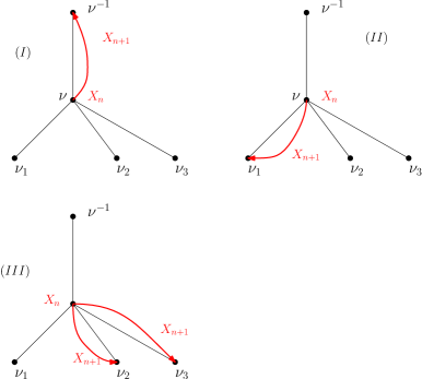
First of all, let us describe the dynamic of this model. If $\bf X$ visits a vertex $\nu$ for the first time, three cases can occur for visiting $\nu_{1}$ (see Figure 1):

• It eats the cookie at $\nu$ and returns to the parent of $\nu$ (i.e. $\nu^{-1}$) with probability $\frac{1}{1+\partial(\nu)\lambda_{1}}$. It then visits $\nu$ for the second time, and goes to $\nu_{1}$ with probability $\frac{\lambda}{1+\partial(\nu)\lambda}$.

• It goes directly to $\nu_{1}$ with probability $\frac{\lambda_{1}}{1+\partial(\nu)\lambda_{1}}$.

• It goes to one of the chidren of $\nu$ except for $\nu_{1}$, with probability $\frac{(\partial\nu-1)\lambda_{1}}{1+\partial(\nu)\lambda_{1}}$. It then visits $\nu$ for the second time, and goes to $\nu_{1}$ with probability $\frac{\lambda}{1+\partial(\nu)\lambda}$.

Figure 1. The movement of $\bf X$ to $\nu_{1}$ after visiting $\nu$.

Now, we introduce a construction of once-excited random walk by using the Rubin’s construction. Let $(\Omega,\mathcal{F},\mathbf{P})$ denote a probability space on which

(7.1) $${\bf Y}=(Y(\nu,\mu,k):(\nu,\mu)\in V^{2},\mbox{with }\nu\sim\mu,\textrm{ and }k\in\mathbb{N})$$

(7.2) $${\bf Z}=(Z(\nu,\mu):(\nu,\mu)\in V^{2},\mbox{with }\nu\sim\mu)$$

are two families of independent mean $1$ exponential random variables, where $(\nu,\mu)$ denotes an ordered pair of vertices. Let

(7.3) $${\bf U}=(U_{\nu}:\nu\in V)$$

is a family of independent uniformly random variables on $[0,1]$ which is independent to $\bf Y$ and $\bf Z$.

For any pair vertices $\nu,\mu\in V$ with $\nu\sim\mu$, we define the following quantities

(7.4) $$r(\nu,\mu)=\left\{\begin{array}[]{cc}&\lambda^{|\nu|-1}\text{, if }\mu<\nu,\\ &\lambda^{|\mu|-1}\text{, if }\nu<\mu.\end{array}\right.$$

Let $\mathcal{T}^{\prime}$ be a sub-tree of $\mathcal{T}$, we define the extension ${\bf X}^{(\mathcal{T}^{\prime})}=(V^{\prime},E^{\prime})$ on $\mathcal{T}^{\prime}$ in the following way. Denote by $\varrho^{\prime}$ the root of $\mathcal{T}^{\prime}$ which be defined as the vertex of $V^{\prime}$ with smallest distance to the root of $\mathcal{T}$. For any family of nonnegative integers $\bar{k}=(k_{\mu})_{\mu:[\nu,\mu]\in E^{\prime}}$, we let

(7.5) $$A^{(\mathcal{T}^{\prime})}_{\bar{k},n,\nu}:=\{{X}^{(\mathcal{T}^{\prime})}_{n}=\nu\}\cap\bigcap_{\mu:[\nu,\mu]\in E^{\prime}}\{\#\{1\leq j\leq n\colon({X}^{(\mathcal{T}^{\prime})}_{j-1},{X}^{(\mathcal{T}^{\prime})}_{j})=(\nu,\mu)\}=k_{\mu}\}.$$

(7.6) $$t_{\nu}(n):=\#\{1\leq j\leq n:X^{(\mathcal{T}^{\prime})}_{j}=\nu\}.$$

(7.7) $$h_{\nu}:=\inf\{i\geq 1:t_{\nu}(i)=2\}.$$

(7.8) $$\widetilde{A}^{(\mathcal{T}^{\prime})}_{\bar{k},n,\nu}:=\{{X}^{(\mathcal{T}^{\prime})}_{n}=\nu\}\cap\bigcap_{\mu:[\nu,\mu]\in E^{\prime}}\{\#\{h_{\nu}\leq j\leq n\colon({X}^{(\mathcal{T}^{\prime})}_{j-1},{X}^{(\mathcal{T}^{\prime})}_{j})=(\nu,\mu)\}=k_{\mu}\}.$$

(7.9) $$\mathcal{I}^{\mathcal{T}}(\nu):=\#\{i\in\{1,2,\cdots,\partial(\nu)\}:\nu_{i}\in V(\mathcal{T}^{\prime})\}.$$

Set ${X}^{(\mathcal{T}^{\prime})}_{0}=\varrho^{\prime}$ and on the event $A^{(\mathcal{T}^{\prime})}_{\bar{k},n,\nu}\cap\{t_{\nu}(n)\leq 1\}$:

• If $U_{\nu}<\frac{1}{1+\partial(\nu)\lambda_{1}}$, then we set ${X}^{(\mathcal{T}^{\prime})}_{n+1}=\nu^{-1}$.

• If   $U_{\nu}\in\left[\frac{1+(j-1)\lambda_{1}}{1+\partial(\nu)\lambda_{1}},\frac{1+j\lambda_{1}}{1+\partial(\nu)\lambda_{1}}\right]$ and $j\in\mathcal{I}^{\mathcal{T}}(\nu)$, then we set $X^{(\mathcal{T^{\prime}})}_{n+1}=v_{j}$.

• If   $U_{\nu}\in\left[\frac{1+(j-1)\lambda_{1}}{1+\partial(\nu)\lambda_{1}},\frac{1+j\lambda_{1}}{1+\partial(\nu)\lambda_{1}}\right]$ for some $j\notin\mathcal{I}^{\mathcal{T}}(\nu)$ and

  $$\left\{\nu^{\prime}=\operatorname*{arg\,min}_{\mu:[\nu,\mu]\in E^{\prime}}\Big{\{}\frac{Z(\nu,\mu)}{r(\nu,\mu}\Big{\}}\right\},$$

  we set $X^{(\mathcal{T^{\prime}})}_{n+1}=\nu^{\prime}$.

On the event

(7.10) $$\widetilde{A}^{(\mathcal{T}^{\prime})}_{\bar{k},n,\nu}\cap\{t_{\nu}(n)\geq 2\}\cap\left\{\nu^{\prime}=\operatorname*{arg\,min}_{\mu:[\nu,\mu]\in E^{\prime}}\Big{\{}\sum_{i=0}^{k_{\mu}}\frac{Y(\nu,\mu,i)}{r(\nu,\mu)}\Big{\}}\right\},$$

we set ${X}^{(\mathcal{T}^{\prime})}_{n+1}=\nu^{\prime}$, where the function $r$ is defined in (7.4) and the clocks $Y$’s are from the same collection ${\bf Y}$ fixed in (7.1).

Thus, this defines ${\bf X}^{(\mathcal{T})}$ as the extension on the whole tree. By using the properties of independent exponential random variables, it is easy to check that this construction is a construction of $(\lambda_{1},\lambda)$-OERW on the tree $\mathcal{T}$. We refer the reader to ([4], section 7) for more discussions on this construction.

In the case $\mathcal{T}^{\prime}=[\varrho,\nu]$ for some vertex $\nu$ of $\mathcal{T}$, we write ${\bf X}^{(\nu)}$ instead of ${\bf X}^{([\varrho,\nu])}$, and we denote $T^{(\nu)}(\cdot)$ the return times associated to ${\bf X}^{(\nu)}$. For simplicity, we will also write ${\bf X}^{(e)}$ and $T^{(e)}(\cdot)$ instead of ${\bf X}^{(e^{+})}$ and $T^{(e^{+})}(\cdot)$ for $e\in E$.

Remark 13.

Let $\mathcal{T}^{\prime}$ be a proper subtree of $\mathcal{T}$. Note that ${\bf X}^{(\mathcal{T}^{\prime})}$ is not $(\lambda_{1},\lambda)$-OERW on $\mathcal{T}^{\prime}$, that is different with $M$-digging random walk (see [4], section 7) and once-reinforced random walk (see [5], section 5).

Finally, we give a probabilistic interpretation of the functions $\phi$ and $\Psi$:

Lemma 14.

For any $e\in E$ and any $g\leq e$, we have

(7.11) $$\phi(g,\lambda_{1},\lambda) =\mathbb{P}\left(T^{(e)}(g^{+})\circ\theta_{T^{(e)}(g^{-})}<T^{(e)}({\varrho})\circ\theta_{T^{(e)}(g^{-})}\right),$$

(7.12) $$\Psi(e,\lambda_{1},\lambda) =\mathbb{P}\left(T^{(e)}(e^{+})<T^{(e)}({\varrho})\right),$$

where $\theta$ is the canonical shift on the trajectories.

Proof.

Let $e\in E$ and $g\leq e$. For simplicity, we set

$$\mathcal{A}:=\{T^{(e)}(g^{+})\circ\theta_{T^{(e)}(g^{-})}<T^{(e)}({\varrho})\circ\theta_{T^{(e)}(g^{-})}\},$$

$$\mathcal{I}_{1}:=\left[\frac{1+(j-1)\lambda_{1}}{1+\partial(g^{-})\lambda_{1}},\frac{1+j\lambda_{1}}{1+\partial(g^{-})\lambda_{1}}\right],$$

$$\mathcal{I}_{2}:=[0,1]\setminus\left(\left[\frac{1+(j-1)\lambda_{1}}{1+\partial(g^{-})\lambda_{1}},\frac{1+j\lambda_{1}}{1+\partial(g^{-})\lambda_{1}}\right]\bigcup\left[0,\frac{1}{1+\partial(g^{-})\lambda_{1}}\right]\right),$$

where $j\in\{1,...,\partial(g^{-})\}$ such that $(g^{-})_{j}=g^{+}$. We have that

(7.13) $$\begin{split}&\mathbb{P}\left(\mathcal{A}\right)=\mathbb{P}\left(A\Big{|}U_{g^{-}}<\frac{1}{1+\partial(g^{-})\lambda_{1}}\right)\times\mathbb{P}\left(U_{g^{-}}<\frac{1}{1+\partial(g^{-})\lambda_{1}}\right)\\ +&\mathbb{P}\left(A|\mathcal{I}_{1}\right)\times\mathbb{P}\left(U_{g^{-}}\in\mathcal{I}_{1}\right)+\mathbb{P}\left(A|\mathcal{I}_{2}\right)\times\mathbb{P}\left(U_{g^{-}}\in\mathcal{I}_{2}\right).\end{split}$$

On the other hand, we have the following equalities:

(7.14) $$\mathbb{P}\left(A\Big{|}U_{g^{-}}<\frac{1}{1+\partial(g^{-})\lambda_{1}}\right)\times\mathbb{P}\left(U_{g^{-}}<\frac{1}{1+\partial(g^{-})\lambda_{1}}\right)=\\ \frac{1}{1+\partial(g^{-})\lambda_{1}}\psi(g,\lambda)\psi(g^{-1},\lambda)$$

(7.15) $$\mathbb{P}\left(A|\mathcal{I}_{1}\right)\times\mathbb{P}\left(U_{g^{-}}\in\mathcal{I}_{1}\right)=\frac{\lambda_{1}}{1+\partial(g^{-})\lambda_{1}}.$$

(7.16) $$\mathbb{P}\left(A|\mathcal{I}_{2}\right)\times\mathbb{P}\left(U_{g^{-}}\in\mathcal{I}_{2}\right)=\frac{(\partial(g^{-})-1)\lambda_{1}}{1+\partial(g^{-})\lambda_{1}}\psi(g,\lambda).$$

We use (7.13), (7.14), (7.15) and (7.16) to obtain the results. ∎

8. Recurrence in Theorem 4: The case $RT(\mathcal{T},{\bf X})<1$

Proposition 15.

If

(8.1) $$\inf_{\pi\in\Pi}\sum_{e\in\pi}\Psi(e)=0,$$

then $\mathbf{X}$ is recurrent.

Proof.

The proof is identical to the proof of Proposition 10 of [5]. ∎

9. Transience in Theorem 4: The case $RT(\mathcal{T},{\bf X})>1$

In order to prove transience, we use the relationship between the walk $\bf{X}$ and its associated percolation.

9.1. Link with percolation

Denote by $C(\varrho)$ the set of edges which are crossed by ${\bf X}$ before returning to $\varrho$, that is:

(9.1) $$\mathcal{C}(\varrho)=\{e\in E:T(e^{+})<T(\varrho)\}.$$

We define an other percolation which will be more easy to study. In order to do this, we use the Rubin’ s construction and the extensions introduced in Section 7. We define

(9.2) $$\mathcal{C}_{CP}(\varrho)=\{e\in E:T^{(e)}(e^{+})<T^{(e)}(\varrho)\}.$$

We say that an edge $e\in E$ is open if and only if $e\in\mathcal{C}_{CP}(\varrho)$.

Lemma 16.

We have that

(9.3) $$\mathbb{P}(T(\varrho)=\infty)=\mathbb{P}(|\mathcal{C}(\varrho)|=\infty)=\mathbb{P}(|\mathcal{C}_{CP}(\varrho)|=\infty).$$

Proof.

We can follow line by line the proof of Lemma 11 in [5]. ∎

For simplicity, for a vertex $v\in V$, we write $v\in\mathcal{C}_{\mathrm{CP}}(\varrho)$ if one of the edges incident to $v$ is in $\mathcal{C}_{\mathrm{CP}}(\varrho)$. Besides, recall that for two edges $e_{1}$ and $e_{2}$, their common ancestor with highest generation is the vertex denoted $e_{1}\wedge e_{2}$.

Lemma 17.

Let $\lambda_{1}\geq 0$, $\lambda>0$ and $\mathcal{T}$ be an infinite, locally finite and rooted tree with the root $\varrho$. Assume that the condition (3.4) holds with some constant $M$. Then the correlated percolation induced by $\mathcal{C}_{CP}$ is quasi-independent, i.e. there exists a constant $C_{Q}\in(0,+\infty)$ such that, for any two edges $e_{1},e_{2}$, we have that

(9.4) $$\begin{split}\mathbb{P}(e_{1},e_{2}\in\mathcal{C}_{CP}(\varrho)|e_{1}\wedge e_{2}\in\mathcal{C}_{CP}(\varrho))\leq&C_{Q}\mathbb{P}(e_{1}\in\mathcal{C}_{CP}(\varrho)|e_{1}\wedge e_{2}\in\mathcal{C}_{CP}(\varrho))\\ &\times\mathbb{P}(e_{2}\in\mathcal{C}_{CP}(\varrho)|e_{1}\wedge e_{2}\in\mathcal{C}_{CP}(\varrho)).\end{split}$$

Proof.

Recall the construction of Section 7. Note that if $e_{1}\wedge e_{2}=\varrho$, then the extensions on $[\varrho,e_{1}]$ and $[\varrho,e_{2}]$ are independent, then the conclusion of Lemma holds with $C=1$. Assume that $e_{1}\wedge e_{2}\neq\varrho$, and note that the extensions on $[\varrho,e_{1}]$ and $[\varrho,e_{2}]$ are dependent since they use the same clocks on $[\varrho,e_{1}\wedge e_{2}]$. Denote by $e$ the unique edge of $\mathcal{T}$ such that $e^{+}=e_{1}\wedge e_{2}$. For $i\in\{1,2\}$, let $v_{i}$ be the vertex which is the offspring of $e^{+}$ lying the path from $\varrho$ to $e_{i}$. Note that $v_{i}$ could be equal to $e^{+}_{i}$. Let $i_{1}$ (resp. $i_{2}$) be an element of $\{1,...,\partial(e^{+})\}$ such that $(e^{+})_{i_{1}}=v_{1}$ (resp. $(e^{+})_{i_{2}}=v_{2}$).
As the events $\{e\in\mathcal{C}_{CP}\}$ and $U_{e_{1}\wedge e_{2}}$ are independent, therefore:

$$\mathbb{P}\left(e_{1},e_{2}\in\mathcal{C}_{CP}(\varrho)|e\in\mathcal{C}_{CP}(\varrho)\right)=A+B+C+D,$$

where

(9.5) $$A=\mathbb{P}\left(e_{1},e_{2}\in\mathcal{C}_{CP}(\varrho)\Big{|}e\in\mathcal{C}_{CP}(\varrho),\,U_{e^{+}}<\frac{1}{1+\partial(e^{+})\lambda_{1}}\right)\mathbb{P}\left(U_{e^{+}}<\frac{1}{1+\partial(e^{+})\lambda_{1}}\right)$$

(9.6) $$\begin{split}B=\mathbb{P}\left(e_{1},e_{2}\in\mathcal{C}_{CP}(\varrho)\Big{|}e\in\mathcal{C}_{CP}(\varrho),\,U_{e^{+}}\in\left[\frac{1+(i_{1}-1)\lambda_{1}}{1+\partial(e^{+})\lambda_{1}},\frac{1+i_{1}\lambda_{1}}{1+\partial(e^{+})\lambda_{1}}\right]\right)\\ \times\mathbb{P}\left(U_{e^{+}}\in\left[\frac{1+(i_{1}-1)\lambda_{1}}{1+\partial(e^{+})\lambda_{1}},\frac{1+i_{1}\lambda_{1}}{1+\partial(e^{+})\lambda_{1}}\right]\right).\end{split}$$

(9.7) $$\begin{split}C=\mathbb{P}\left(e_{1},e_{2}\in\mathcal{C}_{CP}(\varrho)\Big{|}e\in\mathcal{C}_{CP}(\varrho),\,U_{e^{+}}\in\left[\frac{1+(i_{2}-1)\lambda_{1}}{1+\partial(e^{+})\lambda_{1}},\frac{1+i_{2}\lambda_{1}}{1+\partial(e^{+})\lambda_{1}}\right]\right)\\ \times\mathbb{P}\left(U_{e^{+}}\in\left[\frac{1+(i_{2}-1)\lambda_{1}}{1+\partial(e^{+})\lambda_{1}},\frac{1+i_{2}\lambda_{1}}{1+\partial(e^{+})\lambda_{1}}\right]\right).\end{split}$$

(9.8) $$\begin{split}D=\mathbb{P}\left(e_{1},e_{2}\in\mathcal{C}_{CP}(\varrho)\Big{|}e\in\mathcal{C}_{CP}(\varrho),\,U_{e^{+}}\in\bigcup_{i\in\{1,\cdots,\partial(e^{+})\}\setminus\{i_{1},i_{2}\}}\left[\frac{1+(i-1)\lambda_{1}}{1+\partial(e^{+})\lambda_{1}},\frac{1+i\lambda_{1}}{1+\partial(e^{+})\lambda_{1}}\right]\right)\\ \times\mathbb{P}\left(U_{e^{+}}\in\bigcup_{i\in\{1,\cdots,\partial(v)\}\setminus\{i_{1},i_{2}\}}\left[\frac{1+(i-1)\lambda_{1}}{1+\partial(e^{+})\lambda_{1}},\frac{1+i\lambda_{1}}{1+\partial(e^{+})\lambda_{1}}\right]\right).\end{split}$$

In the same way, for any $j\in\{1,2\}$, we have:

$$\mathbb{P}\left(e_{j}\in\mathcal{C}_{CP}(\varrho)|e\in\mathcal{C}_{CP}(\varrho)\right)=E_{j}+F_{j}+G_{j},$$

where

(9.9) $$\begin{split}E_{j}=\mathbb{P}\left(e_{j}\in\mathcal{C}_{CP}(\varrho)\Big{|}e\in\mathcal{C}_{CP}(\varrho),\,U_{e^{+}}<\frac{1}{1+\partial(e^{+})\lambda_{1}}\right)\mathbb{P}\left(U_{e^{+}}<\frac{1}{1+\partial(e^{+})\lambda_{1}}\right)\end{split}$$

(9.10) $$\begin{split}F_{j}=\mathbb{P}\left(e_{j}\in\mathcal{C}_{CP}(\varrho)\Big{|}e\in\mathcal{C}_{CP}(\varrho),\,U_{e^{+}}\in\left[\frac{1+(i_{j}-1)\lambda_{1}}{1+\partial(e^{+})\lambda_{1}},\frac{1+i_{j}\lambda_{1}}{1+\partial(e^{+})\lambda_{1}}\right]\right)\\ \times\mathbb{P}\left(U_{e^{+}}\in\left[\frac{1+(i_{j}-1)\lambda_{1}}{1+\partial(e^{+})\lambda_{1}},\frac{1+i_{j}\lambda_{1}}{1+\partial(e^{+})\lambda_{1}}\right]\right)\end{split}$$

(9.11) $$\begin{split}G_{j}=\mathbb{P}\left(e_{j}\in\mathcal{C}_{CP}(\varrho)\Big{|}e\in\mathcal{C}_{CP}(\varrho),\,U_{e^{+}}\in\bigcup_{i\in\{1,\cdots,\partial(e^{+})\}\setminus\{i_{j}\}}\left[\frac{1+(i-1)\lambda_{1}}{1+\partial(e^{+})\lambda_{1}},\frac{1+i\lambda_{1}}{1+\partial(e^{+})\lambda_{1}}\right]\right)\\ \times\mathbb{P}\left(U_{e^{+}}\in\bigcup_{i\in\{1,\cdots,\partial(e^{+})\}\setminus\{i_{j}\}}\left[\frac{1+(i-1)\lambda_{1}}{1+\partial(e^{+})\lambda_{1}},\frac{1+i\lambda_{1}}{1+\partial(e^{+})\lambda_{1}}\right]\right).\end{split}$$

Lemma 18.

There exists four constants $(\alpha_{1},\alpha_{2},\alpha_{3},\alpha)$ depend on $\mathcal{T}$, $\lambda$ and $\lambda_{1}$ such that:

(9.12) $$A\leq\alpha_{1}E_{1}E_{2}.$$

(9.13) $$B\leq\alpha_{2}F_{1}E_{2}.$$

(9.14) $$C\leq\alpha_{3}F_{2}E_{1}.$$

(9.15) $$D\leq\alpha_{4}G_{1}G_{2}.$$

We deduce from Lemma 18 that

$$A+B+C+D\leq\alpha(E_{1}+F_{1}+G_{1})(E_{2}+F_{2}+G_{2}),$$

where $\alpha=\max_{i\in\{1,2,3,4\}}\alpha_{i}$. The latter inequality concludes the proof of Proposition. ∎

Proof of Lemma 18.

Now, we will adapt the argument from the proof of Lemma 12 in [5]. We prove that there exists $\alpha_{1}$ such that $A\leq\alpha_{1}E_{1}E_{2}$ and we use the same argument for the other inequalities.

First, by using condition 3.4, note that,

$$\mathbb{P}\left(U_{e^{+}}<\frac{1}{1+\partial(e^{+})\lambda_{1}}\right)=\frac{1}{1+\partial(e^{+})\lambda_{1}}\geq\frac{1}{1+M\lambda_{1}},\text{ we then obtain: }$$

(9.16) $$\mathbb{P}\left(U_{e^{+}}<\frac{1}{1+\partial(e^{+})\lambda_{1}}\right)\leq(1+M\lambda_{1})\left[\mathbb{P}\left(U_{e^{+}}<\frac{1}{1+\partial(e^{+})\lambda_{1}}\right)\right]^{2}.$$

On the event $\left\{e\in\mathcal{C}_{CP}(\varrho),\,U_{e^{+}}<\frac{1}{1+\partial(e^{+})\lambda_{1}}\right\}$ we have $X^{(e)}_{T^{(e)}(e^{+})+1}=e^{-}$. We then define $\widetilde{T}^{(e)}(e^{+}):=\inf\left\{n\geq T^{(e)}(e^{+})+1:X^{(e)}_{n}=e^{+}\right\}$. We define the following quantities:

(9.17) $$\begin{split}N(e)&=\left|\left\{\widetilde{T}^{(e)}(e^{+})\leq n\leq T^{(e)}(\varrho)\circ\theta_{\widetilde{T}^{(e)}(e^{+})}:({X}^{(e)}_{n},{X}^{(e)}_{n+1})=(e^{+},e^{-})\right\}\right|,\\ L(e)&=\sum_{j=0}^{N(e)-1}\frac{Y(e^{+},e^{-},j)}{r(e^{+},e^{-})},\end{split}$$

where $|A|$ denotes the cardinality of a set $A$ and $\theta$ is the canonical shift on trajectories. Note that $L(e)$ is the time consumed by the clocks attached to the oriented edge $(e^{+},e^{-})$ before ${\bf X}^{{{\scriptscriptstyle{({e}})}}}$, ${X}^{{{\scriptscriptstyle{({e_{1}}})}}}$ or ${X}^{{{\scriptscriptstyle{({e_{2}}})}}}$ goes back to ${\varrho}$ once it has returned $e^{+}$ after the time $T^{(e)}(e^{+})$. Recall that these three extensions are coupled and thus the time $L(e)$ is the same for the three of them.
For $i\in\{1,2\}$, recall that $v_{i}$ is the vertex which is the offspring of $e^{+}$ lying the path from $\varrho$ to $e_{i}$. Note that $v_{i}$ could be equal to $e^{+}_{i}$. We define for $i\in\{1,2\}$:

(9.18) $$\begin{split}N^{*}(e_{i})&=\left|\left\{\widetilde{T}^{(e)}(e^{+})\leq n\leq T^{(e_{i})}(e_{i}^{+}):({X}^{[e^{+},e_{i}^{+}]}_{n},{X}^{[e^{+},e_{i}^{+}]}_{n+1})=(e^{+},v_{i})\right\}\right|,\\ L^{*}(e_{i})&=\sum_{j=0}^{N^{*}(e_{i})-1}\frac{Y(e^{+},e^{-},j)}{r(e^{+},e^{-})}.\end{split}$$

Here, $L^{*}(e_{i})$, $i\in\{1,2\}$, is the time consumed by the clocks attached to the oriented edge $(e^{+},v_{i})$ before ${\bf X}^{{{\scriptscriptstyle{({e_{i}}})}}}$, or ${\bf X}^{[e^{+},e_{i}^{+}]}$, hits $e_{i}^{+}$.
Notice that the three quantities $L(e)$, $L^{*}(e_{1})$ and $L^{*}(e_{2})$ are independent, and we also have:

(9.19) $$\begin{split}\mathbb{P}\left(e_{1},e_{2}\in\mathcal{C}_{CP}(\varrho)\Big{|}e\in\mathcal{C}_{CP}(\varrho),\,U_{e^{+}}<\frac{1}{1+\partial(e^{+})\lambda_{1}}\right)\\ =\psi(e,\lambda)\mathbb{P}\left(L(e)>L^{*}(e_{1})\vee L^{*}(e_{2})\right).\end{split}$$

(9.20) $$\begin{split}\mathbb{P}\left(e_{1}\in\mathcal{C}_{CP}(\varrho)\Big{|}e\in\mathcal{C}_{CP}(\varrho),\,U_{e^{+}}<\frac{1}{1+\partial(e^{+})\lambda_{1}}\right)=\psi(e,\lambda)\mathbb{P}\left(L(e)>L^{*}(e_{1})\right).\end{split}$$

(9.21) $$\begin{split}\mathbb{P}\left(e_{2}\in\mathcal{C}_{CP}(\varrho)\Big{|}e\in\mathcal{C}_{CP}(\varrho),\,U_{e^{+}}<\frac{1}{1+\partial(e^{+})\lambda_{1}}\right)=\psi(e,\lambda)\mathbb{P}\left(L(e)>L^{*}(e_{2})\right).\end{split}$$

Now, the random variable $N(e)$ is simply a geometric random variable (counting the number of trials) with success probability $\lambda^{1-|e|}/\sum_{g\leq e}\lambda^{1-|g|}$. The random variable $N(e)$ is independent of the family $Y(e^{+},e^{-},\cdot)$. As $Y(e^{+},e^{-},j)$ are independent exponential random variable for $j\geq 0$, we then have that $L(e)$ is an exponential random variables with parameter

(9.22) $$p:=\frac{\lambda^{1-|e|}}{\sum_{g\leq e}\lambda^{1-|g|}}\times\lambda^{|e|-1}=\frac{1}{\sum_{g\leq e}\lambda^{1-|g|}}.$$

A priori, $L^{*}(e_{1})$ and $L^{*}(e_{2})$ are not exponential random variable, but they have a continuous distribution. Denote $f_{1}$ and $f_{2}$ respectively the densities of $L^{*}(e_{1})$ and $L^{*}(e_{2})$. Then, we have that

(9.23) $$\begin{split}\mathbb{P}\left(L(e)>L^{*}(e_{1})\vee L^{*}(e_{2})\right)&=\int_{0}^{+\infty}\int_{0}^{+\infty}\int_{x_{1}\vee x_{2}}^{+\infty}p\,e^{-pt}f_{1}(x_{1})f_{2}(x_{2})dtdx_{1}dx_{2}\\ &=\int_{0}^{+\infty}\int_{0}^{+\infty}e^{{-p}(x_{1}\vee x_{2})}f_{1}(x_{1})f_{2}(x_{2})dx_{1}dx_{2}.\\ &\leq\int_{0}^{+\infty}\int_{0}^{+\infty}e^{\frac{-p}{2}(x_{1}+x_{2})}f_{1}(x_{1})f_{2}(x_{2})dx_{1}dx_{2}.\end{split}$$

Thus, one can write

(9.24) $$\begin{split}&\mathbb{P}\left(L(e)>L^{*}(e_{1})\vee L^{*}(e_{2})\right)\\ &\leq\left(\int_{0}^{+\infty}e^{-px_{1}/2}f_{1}(x_{1})dx_{1}\right)\cdot\left(\int_{0}^{+\infty}e^{-px_{2}/2}f_{2}(x_{2})dx_{2}\right).\end{split}$$

Note that:

(9.25) $$\int_{0}^{+\infty}e^{-px_{1}/2}f_{1}(x_{1})dx_{1}=\mathbb{P}\left(\widetilde{L}(e)>L^{*}(e_{1})\right),$$

where $\widetilde{L}(e)$ is an exponential variable with parameter $p/2$. Note that, in view of (9.22), $\widetilde{L}(e)$ has the same law as $L(e)$ when we replace the weight of an edge $g^{\prime}$ by $\lambda^{-|g^{\prime}|+1}/2$ for $g^{\prime}\leq e$ only, and keep the other weights the same.
For simplicity, for any $g\in E$, we set $w(g)=\lambda^{|g|-1}$. For $g\in E$ such that $e<g$, define the functions $\widetilde{\psi}$ and $\widetilde{\phi}$ in a similar way as $\psi$ and $\phi$, except that we replace the weight of an edge $g^{\prime}$ by $\lambda^{-|g^{\prime}|+1}/2$ for $g^{\prime}\leq e$ only, and keep the other weights the same, that is, for $g\in E$, $e<g$,

(9.26) $$\widetilde{\psi}(g,\lambda)=\frac{\sum_{g^{\prime}<g}w(g^{\prime})^{-1}+\sum_{g^{\prime}\leq e}w(g^{\prime})^{-1}}{\sum_{g^{\prime}\leq g}w(g^{\prime})^{-1}+\sum_{g^{\prime}\leq e}w(g^{\prime})^{-1}}.$$

(9.27) $$\widetilde{\phi}(g,\lambda_{1},\lambda)=\frac{\lambda_{1}}{1+\partial(g^{-})\lambda_{1}}+\frac{1}{1+\partial(g^{-})\lambda_{1}}\widetilde{\psi}(g,\lambda)\widetilde{\psi}(g^{-1},\lambda)+\frac{(\partial(g^{-})-1)\lambda_{1}}{1+\partial(g^{-})\lambda_{1}}\widetilde{\psi}(g,\lambda).$$

We obtain:

(9.28) $$\begin{split}&\mathbb{P}(\widetilde{L}(e)>L^{*}(e_{1}))=\prod_{e<g\leq e_{1}}\widetilde{\phi}(g,\lambda_{1},\lambda)=\prod_{e<g\leq e_{1}}\phi(g,\lambda_{1},\lambda)\prod_{e<g\leq e_{1}}\left(\frac{\widetilde{\phi}(g,\lambda_{1},\lambda)}{\phi(g,\lambda_{1},\lambda)}\right)\\ &=\mathbb{P}(L(e)>L^{*}(e_{1}))\times\prod_{e<g\leq e_{1}}\left(\frac{\lambda_{1}+\widetilde{\psi}(g,\lambda)\widetilde{\psi}(g^{-1},\lambda)+(\partial(g^{-1})-1)\lambda_{1}\widetilde{\psi}(g,\lambda)}{\lambda_{1}+\psi(g,\lambda)\psi(g^{-1},\lambda)+(\partial(g^{-1})-1)\lambda_{1}\psi(g,\lambda)}\right)\\ &=\mathbb{P}(L(e)>L^{*}(e_{1}))\\ &\qquad\times\prod_{e<g\leq e_{1}}\left(1+\frac{\widetilde{\psi}(g,\lambda)\widetilde{\psi}(g^{-1},\lambda)-\psi(g,\lambda)\psi(g^{-1},\lambda)+(\partial(g^{-1})-1)\lambda_{1}(\widetilde{\psi}(g,\lambda)-\psi(g,\lambda))}{\lambda_{1}+\psi(g,\lambda)\psi(g^{-1},\lambda)+(\partial(g^{-1})-1)\lambda_{1}\psi(g,\lambda)}\right).\end{split}$$

Now, we compute the product:

$$\prod_{e<g\leq e_{1}}\left(1+\frac{\widetilde{\psi}(g,\lambda)\widetilde{\psi}(g^{-1},\lambda)-\psi(g,\lambda)\psi(g^{-1},\lambda)+(\partial(g^{-1})-1)\lambda_{1}(\widetilde{\psi}(g,\lambda)-\psi(g,\lambda))}{\lambda_{1}+\psi(g,\lambda)\psi(g^{-1},\lambda)+(\partial(g^{-1})-1)\lambda_{1}\psi(g,\lambda)}\right)$$

$$\leq\prod_{e<g\leq e_{1}}\left(1+\frac{\widetilde{\psi}(g,\lambda)\widetilde{\psi}(g^{-1},\lambda)-\psi(g,\lambda)\psi(g^{-1},\lambda)+(\partial(g^{-1})-1)\lambda_{1}(\widetilde{\psi}(g,\lambda)-\psi(g,\lambda))}{\lambda_{1}}\right).$$

$$\leq\exp{\left(\frac{1}{\lambda_{1}}\sum_{e<g\leq e_{1}}\left(\widetilde{\psi}(g,\lambda)\widetilde{\psi}(g^{-1},\lambda)-\psi(g,\lambda)\psi(g^{-1},\lambda)+(\partial(g^{-1})-1)\lambda_{1}(\widetilde{\psi}(g,\lambda)-\psi(g,\lambda))\right)\right)}$$

Lemma 19.

There exists a constant $c=c(\lambda_{1},\lambda)$ which do not depend on $e$, $e_{1}$ and $e_{2}$, such that:

(9.29) $$\sum_{e<g\leq e_{1}}\left(\widetilde{\psi}(g,\lambda)-\psi(g,\lambda)\right)\leq c.$$

On the other hand, by using Lemma 19, for any $e$ and $e_{1}$ we have that

(9.30) $$\sum_{e<g\leq e_{1}}\left(\widetilde{\psi}(g,\lambda)\widetilde{\psi}(g^{-1},\lambda)-\psi(g,\lambda)\psi(g^{-1},\lambda)\right)\leq 2c.$$

By using 9.30, Lemma 19 and condition (3.4), we obtain:

(9.31) $$\begin{split}&\prod_{e<g\leq e_{1}}\left(1+\frac{\widetilde{\psi}(g,\lambda)\widetilde{\psi}(g^{-1},\lambda)-\psi(g,\lambda)\psi(g^{-1},\lambda)+(\partial(g^{-1})-1)\lambda_{1}(\widetilde{\psi}(g,\lambda)-\psi(g,\lambda))}{\lambda_{1}+\psi(g,\lambda)\psi(g^{-1},\lambda)+(\partial(g^{-1})-1)\lambda_{1}\psi(g,\lambda)}\right)\\ &\leq\exp\left(Mc+\frac{2c}{\lambda_{1}}\right).\end{split}$$

We have just proved that

(9.32) $$\int_{0}^{+\infty}e^{-px_{1}/2}f_{1}(x_{1})dx_{1}\leq\exp\left(Mc+\frac{2c}{\lambda_{1}}\right)\times\mathbb{P}(e_{1}\in\mathcal{C}_{CP}(\varrho)|e_{1}\wedge e_{2}\in\mathcal{C}_{CP}(\varrho)).$$

By doing a very similar computation, one can prove that

(9.33) $$\int_{0}^{+\infty}e^{-px_{2}/2}f_{1}(x_{2})dx_{2}\leq\exp\left(Mc+\frac{2c}{\lambda_{1}}\right)\times\mathbb{P}(e_{2}\in\mathcal{C}_{CP}(\varrho)|e_{1}\wedge e_{2}\in\mathcal{C}_{CP}(\varrho)).$$

Moreover, we have

(9.34) $$\psi(e,\lambda)\geq\frac{\lambda}{1+\lambda}.$$

The conclusion (9.4) follows by using (9.16), (9.24), (9.34), together with (9.32) and (9.33). ∎

It remains to prove Lemma 19.

Proof of Lemma 19.

By a simple computation, for any $e<g\leq e_{1}$,

(9.35) $$\begin{split}&\widetilde{\psi}(g,\lambda)-\psi(g,\lambda)=\frac{\left(\sum_{g^{\prime}\leq e}w(g^{\prime})^{-1}\right)w(g)^{-1}}{\left(\sum_{g^{\prime}\leq g}w(g^{\prime})^{-1}+\sum_{g^{\prime}\leq e}w(g^{\prime})^{-1}\right)\left(\sum_{g^{\prime}\leq g}w(g^{\prime})^{-1}\right)}.\end{split}$$

We will proceed by distinguishing three cases.
Case I: $\lambda<1$.
By (9.35), we have that

(9.36) $$\begin{split}&\widetilde{\psi}(g,\lambda)-\psi(g,\lambda)=\frac{\left(1-\frac{1}{\lambda^{|e|}}\right)\frac{1}{\lambda^{|g|-1}}}{\left(1-\frac{1}{\lambda^{|g|}}+1-\frac{1}{\lambda^{|e|}}\right)\left(1-\frac{1}{\lambda^{|g|}}\right)}\times\left(1-\frac{1}{\lambda}\right).\end{split}$$

Hence, there exists a constants $c_{1}$ such that

(9.37) $$0\leq\widetilde{\psi}(g,\lambda)-\psi(g,\lambda)\leq c_{1}\lambda^{|g|-|e|}.$$

Therefore we obtain

(9.38) $$\sum_{e<g\leq e_{1}}\left(\widetilde{\psi}(g,\lambda)-\psi(g,\lambda)\right)\leq c_{1}\sum_{e<g\leq e_{1}}\lambda^{|g|-|e|}\leq c_{1}\sum_{i\geq 0}\lambda^{i}<\infty.$$

Case II: $\lambda=1$.
By (9.35), we have that

(9.39) $$\widetilde{\psi}(g,\lambda)-\psi(g,\lambda)=\frac{|e|}{|g|(|g|+|e|)}.$$

Therefore we obtain

(9.40) $$\begin{split}&\sum_{e<g\leq e_{1}}\left(\widetilde{\psi}(g,\lambda)-\psi(g,\lambda)\right)\leq\sum_{n\geq|e|}\left(\frac{|e|}{n(n+|e|)}\right)\leq\sum_{n\geq|e|}\left(\frac{1}{n}-\frac{1}{n+|e|}\right)\\ &\leq\sum_{n=|e|}^{2|e|-1}\frac{1}{n}.\end{split}$$

On the other hand, we have:

(9.41) $$\lim_{n\rightarrow\infty}\left(\sum_{k=n}^{2n-1}\frac{1}{k}\right)=\lim_{k\rightarrow\infty}\left(\sum_{k=0}^{n-1}\frac{1}{n+k}\right)=\lim_{k\rightarrow\infty}\left(\frac{1}{n}\sum_{k=0}^{n-1}\frac{1}{1+k/n}\right)=\int_{0}^{1}\frac{dx}{1+x}.$$

We use (9.40) and (9.41) to obtain the result.

Case III: $\lambda>1$.
By (9.35), we have that

(9.42) $$\begin{split}&\widetilde{\psi}(g,\lambda)-\psi(g,\lambda)=\frac{\left(1-\frac{1}{\lambda^{|e|}}\right)\frac{1}{\lambda^{|g|-1}}}{\left(1-\frac{1}{\lambda^{|g|}}+1-\frac{1}{\lambda^{|e|}}\right)\left(1-\frac{1}{\lambda^{|g|}}\right)}\times\left(1-\frac{1}{\lambda}\right).\end{split}$$

Hence, there exists a constants $c_{2}$ such that

(9.43) $$0\leq\widetilde{\psi}(g,\lambda)-\psi(g,\lambda)\leq\frac{c_{2}}{\lambda^{|g|}}.$$

Therefore we obtain

(9.44) $$\sum_{e<g\leq e_{1}}\left(\widetilde{\psi}(g,\lambda)-\psi(g,\lambda)\right)\leq c_{2}\sum_{e<g\leq e_{1}}\frac{1}{\lambda^{|g|}}\leq c_{2}\sum_{i\geq 0}\left(\frac{1}{\lambda}\right)^{i}<\infty.$$

∎

9.2. Transience in Theorem 4: The case $RT(\mathcal{T},{\bf X})>1$

Proposition 20.

If $RT(\mathcal{T},\mathbf{X})>1$ and if (3.4) is satisfied then ${\bf X}$ is transient.

Proof.

The proof is now easy, we can follow line by line the Appendix A.2 of [4]. ∎

10. Proof of Theorem 6

This section is independent with the previous sections. In this section, we prove a criterion which can apply to the critical $M$-digging random walk on superperiodic trees. We will use the Rubin’s construction (resp. the definition of $\mathcal{C}(\varrho)$, $\mathcal{C}_{CP}(\varrho)$) from section 7 (resp. section 8.1) of [4]. We will allow ourselves to omit these definitions and refer the readers to [4] for more details.

The main idea for the proof of Theorem 6 is that the number of surviving rays of the percolation $\mathcal{C}_{CP}(\varrho)$ almost surely is either zero or infinite. This property was proved in the case of Bernoulli percolation (see [8] proposition 5.27) or target percolation (see [10], lemma 4.2). The main difficulty that we have to face is that the FKG inequality is not true for our percolation.

10.1. Some definitions

Let $\lambda>0$, $M\in\mathbb{N}$ and $\mathcal{T}$ be an infinite, locally finite and rooted tree. For each $v\in V(\mathcal{T})$, recall the definition of subtree $\mathcal{T}^{v}$ of $\mathcal{T}$ from Section 2.1. Let ${\bf X}^{v,\lambda}$ be the $M$-digging random walk on $\mathcal{T}^{v}$. We say that $\mathcal{T}$ is uniformly transient if for any $\lambda$ such that the $M$-digging random walk on $\mathcal{T}$ with parameter $\lambda$ is transient (i.e. ${\bf X}^{\varrho,\lambda}$ is transient),

(10.1) $$\exists\alpha_{\lambda}>0,\forall v\in V(\mathcal{T}),\mathbb{P}(\forall n>0,X^{v,\lambda}_{n}\neq v)\geq\alpha_{\lambda}.$$

It is called weakly uniformly transient if there exists a sequence of finite pairwise disjoint $\pi_{n}$ such that

(10.2) $$\exists\alpha_{\lambda}>0,\forall v\in\underset{n}{\bigcup}V(\pi_{n}),\mathbb{P}(\forall n>0,X^{v,\lambda}_{n}\neq v)\geq\alpha_{\lambda}$$

where $V(\pi_{n})=\{e^{-}:e\in\pi_{n}\}$.

Remark 21.

• If $\mathcal{T}$ is uniformly transient, then $\mathcal{T}$ is also weakly uniformly transient, but the reverse is not always true.

• The superperiodic trees are uniformly transient.

An infinite self-avoiding path starting at $\varrho$ is called a ray. The set of all rays, denoted by $\partial\mathcal{T}$, is called the boundary of $\mathcal{T}$. Let $\phi:\mathbb{Z}^{+}\rightarrow\mathbb{R}$ be a decreasing positive function with $\phi(n)\rightarrow 0$ as $n\rightarrow\infty$. The Hausdorff mearsure of $\mathcal{T}$ in gauge $\phi$ is

$$\liminf_{\Pi}\sum_{v\in\Pi}\phi(|v|),$$

where the $\liminf$ is taken over $\Pi$ such that the distance from $\varrho$ to the nearest vertex in $\Pi$ goes to infinity. We say that $\mathcal{T}$ has $\sigma$-finite Hausdorff measure in gauge $\phi$ if $\partial\mathcal{T}$ is the union of countably many subsets with finite Hausdorff measure in gauge $\phi$.

Finally, If $\lambda$ is such that the $M$-digging random walk $X$ with parameter $\lambda$ on $\mathcal{T}$ is transient, on the event $\{T(\varrho)=\infty\}$, its path determines an infinite branch in $\mathcal{T}$, which can be seen as a random ray $\omega^{\infty}$, and call it the limit walk of $X$. Equivalently, on the event $\{T(\varrho)=\infty\}$, we define the limit walk as follows: For any $k\geq 1$,

(10.3) $$\omega^{\infty}(k)=v\iff v\in\mathcal{T}_{k}\text{\leavevmode\nobreak\ and\leavevmode\nobreak\ }\exists n_{0},\forall n>n_{0}:X_{n}\in\mathcal{T}^{v}.$$

Note that $\mathbb{P}\left(\omega^{\infty}(0)=\varrho\right)=1$. For any $k\geq 1$, we call the $k$-first steps of $\omega^{\infty}$ is $(\omega^{\infty}(0),\cdots,\omega^{\infty}(k))$, denoted by $\omega^{\infty}_{|{[0,n]}}$.

10.2. Proof of Theorem 6

Figure 2. The proof’s idea of Proposition 22. The limit walk $\omega^{\infty}$ is in red. Conditioning on the event $\{\omega^{\infty}(0)=\varrho,\omega^{\infty}(1)=v_{1},...,\omega^{\infty}(6)=v_{6}\}$ and denote by $\ell$ the last time the critical $M$-digging random walk ${\bf X}$ on $\mathcal{T}$ visits $v_{6}$. For each $1\leq i\leq 6$, running the walk ${\bf X}^{v_{i},\lambda_{c}}$ on $\mathcal{T}^{v_{i}}$. The property of uniformly transient implies that there exists a surviving ray (in green) in $\mathcal{T}^{v_{i}}$ with probability is larger than a constant which do not depend on $i$.

We begin with the following proposition:

Proposition 22.

Let $\bf X$ be a $M$-digging random walk with parameter $\lambda_{c}$ on an uniformly transient tree $\mathcal{T}$ and recall the definition of $\mathcal{C}_{CP}$ from $\bf X$ as in ([4], Section 7). Consider the percolation induced by $\mathcal{C}_{CP}$ and let $\phi(n)=\mathbb{P}(\varrho\leftrightarrow v)$ for $v\in\mathcal{T}_{n}$.

1. Almost surely, the number of surviving rays is either zero or infinite.

2. If $\partial\mathcal{T}$ has $\sigma$-finite Hausdorff measure in the gauge $\{\phi(n)\}$, then $\mathbb{P}(\varrho\leftrightarrow\infty)=0$. In particular, $\bf X$ is recurrent.

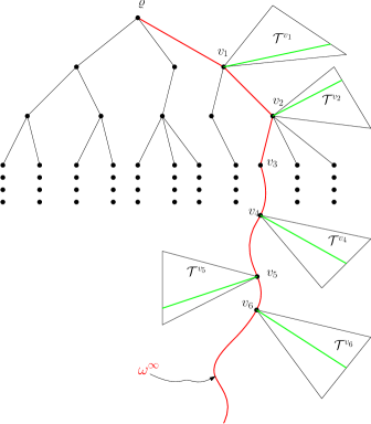
The overall strategy for the proof of Proposition 22 is as follows. First, if ${\bf X}$ is recurrent, then the percolation induced by $\mathcal{C}_{CP}$ almost surely have no surviving ray. Next, assume that ${\bf X}$ is transient. On the event $\left\{T(\varrho)=\infty\right\}$, the limit walk $\omega^{\infty}$ is a surviving ray of $\mathcal{C}_{CP}(\varrho)$. Given $n\in\mathbb{N}$ and conditioning on $\omega^{\infty}_{|{[0,n]}}$, by using the Rubin’s construction and the definition of uniformly transient, we prove that there exists a surviving ray in $\mathcal{T}^{\omega^{\infty}(i)}$ with probability larger than a constant $c$ which do not depend on $i$ and $\omega^{\infty}$ (see Figure 2). The following basic lemma is necessary:

Lemma 23.

Let $\lambda>0$ and $\mathcal{T}$ be an infinite, locally finite and rooted tree. Let $\overline{M}:=(m_{v},v\in V(\mathcal{T}))$ be a family of non-negative integers. Denote by $\bf X$ the $M$-digging random walk with parameter $\lambda$ and $\bf Y$ the $\overline{M}$-digging random walk associated with the inhomogeneous initial number of cookies $\overline{M}$ with parameter $\lambda$ (see [4], section 2.3.2 for more details on the definition of $\overline{M}$-digging random walk). Denote by $T^{\bf X}(\varrho)$ (resp. $T^{\bf Y}(\varrho)$) the return time of $\bf X$ (resp. $\bf Y$) to $\varrho$. Assume that $m(v)\leq M$ for all $v\in V(\mathcal{T})$, we then have

(10.4) $$\mathbb{P}\left(T^{\bf X}(\varrho)<\infty\right)\leq\mathbb{P}\left(T^{\bf Y}(\varrho)<\infty\right).$$

Proof.

The proof is simple, therefore it is omitted. ∎

Proof of Proposition 22.

Let $\mathcal{A}_{k}$ denote the event that exactly $k$ rays survive and assume that

(10.5) $$\mathbb{P}(\mathcal{A}_{k})>0,$$

Hence,

(10.6) $$P(|\mathcal{C}_{CP}(\varrho)|=\infty)>0.$$

By (10.6) and Lemma 22 in [4], we have that:

(10.7) $$\mathbb{P}(T(\varrho)=\infty)>0,$$

and therefore $\bf X$ is transient.

On the event $\{T(\varrho)=\infty\}$, the limit walk $\omega^{\infty}$ of $\bf X$ is well defined and it is a surviving ray. Let $n$ be a positive integer and $\gamma:=(\gamma_{0}=\varrho,\gamma_{1}=v_{1},\cdots,\gamma_{n}=v_{n})$ be a path of length $n$ of $\mathcal{T}$. Denote by $B_{n,\gamma}$ the following event:

(10.8) $$\mathcal{B}_{n,\gamma}:=\{\omega^{\infty}_{|{[0,n]}}=\gamma\}.$$

For any $1\leq k\leq n$, define a sub-tree $\mathcal{T}^{v_{i}}$ of $\mathcal{T}$ in the following way (see Figure 2).

• The root of $\mathcal{T}^{v_{i}}$ is the vertex $v_{i}$.

• If $\partial(v_{i})<2$ then $\mathcal{T}^{v_{i}}$ is a tree with a single vertex $v_{i}$: for example, $\mathcal{T}^{v_{3}}$ in Figure 2.

• If $\partial(\gamma_{i})\geq 2$, choose one of its children which is different to $v_{i+1}$, denoted by $v$. We then set:

  $$\left\{\begin{matrix}(\mathcal{T}^{v_{i}})_{1}=\{v\}\\ (\mathcal{T}^{v_{i}})^{v}=\mathcal{T}^{v}\end{matrix}\right.$$

Note that for every pair $(i,j)\in[1,n]^{2}$, we have $V(\mathcal{T}^{v_{i}})\cap V(\mathcal{T}^{v_{j}})=\varnothing$.

Now, conditioning on the event $\mathcal{B}_{n,\gamma}$. Let $\ell$ be the last time ${\bf X}$ visits $v_{n}$, i.e.

(10.9) $$\ell:=\sup\{k>0:X_{k}=v_{n}\}.$$

By the definition of limit walk, $\ell$ is finite on the event $\mathcal{B}_{n,\gamma}$. For each $i\in[1,n]$ and for all $v\in V(\mathcal{T}^{v_{i}})$, denote by $m^{i}(v)$ the remaining number of cookies at $v$ after time $\ell$, i.e.

(10.10) $$m^{i}(v):=M-\#\{k\leq\ell:X_{k}=v\}.$$

By using the extensions introduced in ([4], Section 7), the next steps on the tree $\mathcal{T}^{v_{i}}$ are given by the digging random walk associated with the inhomogeneous initial number of cookies $(m^{i}(v),v\in V(\mathcal{T}^{v_{i}}))$ and the same parameter $\lambda_{c}$ as $\bf X$, denoted by ${\bf{X}}^{v_{i},m^{i},\lambda_{c}}$ (see [4], section 2.3.2 for more details on the definition of ${\bf{X}}^{v_{i},m^{i},\lambda_{c}}$). Denote by $T^{v_{i},m^{i},\lambda_{c}}$ the return time of ${\bf{X}}^{v_{i},m^{i},\lambda_{c}}$ to the root $v_{i}$ of $\mathcal{T}^{v_{i}}$. By the definition of uniformly transient and Lemma 23, there exists a constant $c>0$ which do not depend on $n$ and $\gamma$ such that for any $i$,

(10.11) $$\mathbb{P}\left(T^{v_{i},m^{i},\lambda_{c}}<\infty\right)>c.$$

On the event $\{T^{v_{i},m^{i},\lambda_{c}}<\infty\}$, note that $\mathcal{C}_{CP}$ contains a surviving ray in $\mathcal{T}^{v_{i}}$. By (10.11), we have

(10.12) $$\mathbb{P}(\mathcal{A}_{k}|\mathcal{B}_{n,\gamma})\leq\binom{n}{k}(1-c)^{n-k}$$

On the other hand, we have $\mathcal{A}_{k}\subset\bigcup_{\gamma:|\gamma|=n}\mathcal{B}_{n,\gamma}$, therefore by (10.12) we obtain:

(10.13) $$\mathbb{P}(\mathcal{A}_{k})=\sum_{\gamma:|\gamma|=n}\mathbb{P}(\mathcal{A}_{k}|\mathcal{B}_{n,\gamma})\times\mathbb{P}(\mathcal{B}_{n,\gamma})\leq\left(\sum_{i=1}^{k}\binom{n}{i}\right)(1-c)^{n}\underbrace{\sum_{\gamma:|\gamma|=n}\mathbb{P}(\mathcal{B}_{n,\gamma})}_{\leq 1}\leq\left(\sum_{i=1}^{k}\binom{n}{i}\right)(1-c)^{n}.$$

Since 10.13 holds for any $n$ then we obtain the following contradiction

(10.14) $$\mathbb{P}(\mathcal{A}_{k})=0.$$

For part (2), the proof is similar to part (ii), Lemma 4.2 in [10]. ∎

In the same method as in the proof of Proposition 22, we can prove the slightly stronger result (the proof of which we omit):

Proposition 24.

Let $\bf X$ be a $M$-digging random walk with parameter $\lambda_{c}$ on a weakly uniformly transient tree $\mathcal{T}$ and recall the definition of $\mathcal{C}_{CP}$ from $\bf X$ as in ([4], Section 7). Consider the percolation induced by $\mathcal{C}_{CP}$ and let $\phi(n)=\mathbb{P}(\varrho\leftrightarrow v)$ for $v\in\mathcal{T}_{n}$.

1. With probability one, the number of surviving rays is either zero or infinite.

2. If $\partial\mathcal{T}$ has $\sigma$-finite Hausdorff measure in the gauge $\{\phi(n)\}$, then $\mathbb{P}(\varrho\leftrightarrow\infty)=0$. In particular, $\bf X$ is recurrent.

The following corollary is an immediate consequence of Proposition 24.

Corollary 25.

Let $M\in\mathbb{N}$ and $\mathcal{T}$ be a weakly uniformly transient tree such that $\partial\mathcal{T}$ has $\sigma$-finite Hausdorff measure in the gauge $\{\phi(n)\}=\left(\frac{1}{br(\mathcal{T})}\right)^{n}$ if $br(\mathcal{T})>1$ and $\{\phi(n)\}=\frac{1}{n^{M+1}}$ if $br(\mathcal{T})=1$. Then the critical $M$-digging random walk on $\mathcal{T}$ is recurrent.

Proposition 26.

Let $M\in\mathbb{N}^{*}$ and $\mathcal{T}$ be a superperiodic tree whose upper-growth rate is finite. The critical $M$-digging random walk on $\mathcal{T}$ is recurrent.

Proof.

This is a consequence of Corollary 25 and Theorem 3. ∎

Remark 27.

If $M=0$, then $M$-DRW_λ is the biased random walk with parameter $\lambda$. The recurrence of critical biased random walk on $\mathcal{T}$ is a consequence of Theorem 3 and Nash-Williams criterion (see [8] or [9]).

Acknowledgement.

I am grateful to Daniel Kious and Andrea Collevecchio for precious discussions. I am thankful to Vincent Beffara for his support.

References

- [1] Basdevant, A.-L. and Singh, A. (2009). Recurrence and transience of a multi-excited random walk on a regular tree, Electron. J. Probab. 14(55), 1628–1669.
- [2] Beffara, V. and Huynh, C. B.(2017). Trees of self-avoiding walks. preprint, arXiv:1711.05527.
- [3] Collevecchio, A., Holmes, M. and Kious, D. (2018). On the speed of once-reinforced biased random walk on trees. Electron. J. Probab. 23(86).
- [4] Collevecchio, Andrea and Huynh, Cong Bang and Kious, Daniel. (2018). The branching-ruin number as critical parameter of random processes on trees. arXiv preprint arXiv:1811.08058.
- [5] Collevecchio, A., Kious, D. and Sidoravicius, V. (2017) The branching-ruin number and the critical parameter of once-reinforced random walk on trees, preprint, arXiv:1710.00567.
- [6] Furstenberg, H. (1970) Intersections of Cantor sets and transversality of semigroups. In Gunning, R.C., editor, Problems in Analysis, pages 41–59. Princeton University Press, Princeton, NJ. A symposium in honor of Salomon Bochner, Princeton University, Princeton, NJ, 1–3 April 1969. MR: 50:7040
- [7] Lyons, R. (1990). Random walks and percolation on trees. Ann. Probab. 18(3), 931–958
- [8] Lyons, R. and Peres Y. (2016). Probability on trees and networks. Cambridge University Press, New York. Pages xvi+699. Available at http://pages.iu.edu/~rdlyons/.
- [9] Nash-Williams, C St JA. (1959). Random walk and electric currents in networks, Mathematical Proceedings of the Cambridge Philosophical Society. 55(02), 181–194.
- [10] Pemantle, Robin and Peres, Yuval. (1995). Critical random walk in random environment on trees. The Annals of Probability., 105–140.
- [11] Volkov, S. (2003) Excited random walk on trees, Electron. J. Probab. 8(23).