Dipole Distortions in the Intergalactic Medium

Abstract

Baryonic feedback can significantly modify the spatial distribution of matter on small scales and create a bulk relative velocity between the dominant cold dark matter and the hot gas. We study the consequences of such bulk motions using two high resolution hydrodynamic simulations, one with no feedback and one with very strong feedback. We find that relative velocities of order $100\ {\rm km}/{\rm s}$ are produced in the strong feedback simulation whereas it is much smaller when there is no feedback. Such relative motions induce dipole distortions to the gas, which we quantify by computing the dipole correlation function. We find halo coordinates and velocities are systematically changed in the direction of the relative velocity. Finally, we discuss potential to observe the relative velocity via large scale structure, Sunyaev-Zel’dovich and line emission measurements. Given the nonlinear nature of this effect, it should next be studied in simulations with different feedback implementations/strengths to determine the available model space.

1 Introduction

The $\Lambda$CDM model of cosmology is now well established, despite its two featured ingredients being dark and mysterious. The observed accelerated expansion of the Universe implies there must be a dark energy that behaves at least somewhat like a cosmological constant. There must also be highly clustered dark matter whose dynamics are mostly similar to those of a perfectly cold kinetic particle except perhaps at the smallest scales. From this perspective, there is then very little about the macroscopic Universe we don’t understand since these two components make up $95\%$ of its energy.

Fortunately, the luminous $5\%$ of the Universe, the baryons, provides a host of their own mysteries. Observations of galaxies and their stars tells us that the stellar matter can only account for $\sim 10\%$ of the baryonic matter and the location of the remaining $\sim 90\%$, and why it isn’t in stars, constitutes the “missing baryons problem.” Galactic feedback processes, which can heat and expel baryons as a warm-hot intergalactic medium, are thought to resolve this problem (Tornatore et al., 2010). We believe that feedback comes mainly in two flavors, arising from different physical processes and involving different energy scales. On one hand, supernova feedback involves small scales and is responsible for the suppression of the stellar mass function for small galaxies. On the other, Active Galactic Nuclei (AGN) feedback operates on large scales and is commonly believed to be the mechanism responsible for the stellar mass function suppression for large galaxies.

Unfortunately, we do not have a complete physical understanding of these phenomena. In cosmological hydrodynamic simulations the large range of scales involved do not allow us to simulate these processes directly and instead subgrid models have been developed to capture them in a phenomenological, but physically motivated, manner (see the Horizon (Dubois et al., 2014), Illustris (Vogelsberger et al., 2014a), IllustrisTNG (Pillepich et al., 2018) or Eagle (Schaye et al., 2015) simulations as relevant examples). The “missing baryons” can then be found in simulations. As an example, Haider et al. (2016) found that around one quarter of baryons end up in halos, just under a half in filaments, and nearly a third in voids. These fractions are not replicated without feedback where more baryons end up in halos. Additionally, the large numbers of void baryons was found to be due to feedback.

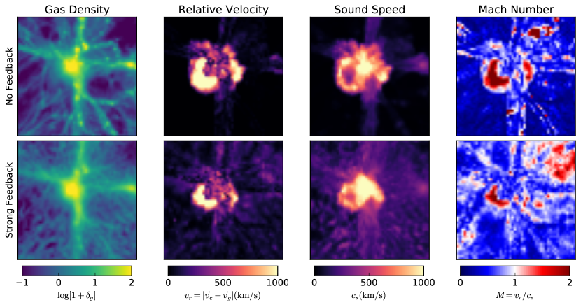
Figure 1: Slices of the gas density, the modulus of the relative velocity, sound speed and Mach number. The slices shown here are at redshift $0$ and have lengths of $39$ Mpc/h and depth $4$ Mpc/h. The upper row corresponds to a simulation with no feedback whereas the bottom row has $50\times$ enhanced feedback. When feedback is strong, the central halo can expel gas, leading to large relative velocities outside the halo.

On the other hand, these feedback processes will affect not just the host galaxy (and halo) itself, but can propagate through the entire intergalactic medium (IGM) as well (Vogelsberger et al., 2014b). We can therefore attempt to learn about feedback through the study of large scale structure via standard clustering statistics such as the power spectrum in Fourier space or correlation function in configuration space (Springel et al., 2017). An alternative possibility is to look for direct dynamical consequences of feedback: energy injection and subsequent heating of the IGM, alongside ejection of the gas out of galaxies. These effects introduce a scale below which there can be a relative velocity between the cold dark matter (CDM) and the gas. A halo moving through the gas will then induce a dipolar density distortion which can then back react and slow down the CDM.

This paper explores the consequences of the relative velocity between the baryons and CDM, as a function of feedback energy. We study this effect by running two simulations with the same initial conditions and gravitational evolution, but differing strength of feedback. We find that the feedback induced relative velocity is largest at redshift $1$, and use this as our fiducial redshift. We begin by quantifying the dipole distortion in the IGM by computing the “dipole correlation function”. We then compute the backreaction effect by comparing individual halos in the two simulations. Finally, we discuss how this feedback driven effect can potentially be observed using measurements of the Sunyaev-Zel’dovich effect, X-ray emission and nonlinear reconstruction.

This paper is organized as follows. In section 2 we describe the hydrodynamic simulations we have run, and the method employed to compute the density, velocity and sound speed fields. We present the main results in section 3 and we draw and discuss the main conclusions of this work in section 5.

2 Simulations

We run high resolution hydrodynamic simulations using the SPH-TreePM code Gadget-III (see Springel et al. (2001) and Springel (2005) for descriptions of previous versions of the code) containing $1024^{3}$ cold dark matter particles and $1024^{3}$ baryonic Smooth-Particle Hydrodynamic (SPH) gas particles in a box of side length $200\ \mbox{Mpc}/\mbox{h}$. Our cosmological parameters are consistent with Planck cosmology: $\Omega_{m}=0.3175$, $\Omega_{\Lambda}=1-\Omega_{m}=0.6825$, $n_{s}=0.9625$, $h=0.6711$ and $\sigma_{8}=0.834$ (Planck Collaboration et al., 2018). The initial conditions have been generated at $z=99$ by displacing the positions of CDM and baryons from two uniform, but offset with respect to one another, grids using the Zel’dovich approximation. We take into account that the growth factors/rates of both components are different when computing the initial displacements and peculiar velocities (Schmidt, 2016; Valkenburg & Villaescusa-Navarro, 2017; Zennaro et al., 2017). The $z=0$ matter power spectra and transfer functions are computed using CAMB (Lewis et al., 2000).

Our simulations include radiative cooling by hydrogen and helium and heating by a uniform UV background. They account for both star formation and supernova feedback as described in Springel & Hernquist (2003). Stellar winds are ejected isotropically from a star particle. The parameter we vary between simulations is the efficiency of the feedback, $\chi$, which describes the fraction of supernova energy which goes into winds. Nominally $\chi\leq 1$; on the other hand, we expect that the kinetic winds underestimate the energy of real galactic feedback which are also driven by AGN. We therefore allow $\chi$ to exceed $100\%$ efficiency and use $\chi=0$ and $\chi=50$, which we will refer to as “no feedback” and “strong feedback” respectively. The corresponding wind speeds are given by $v_{w}(\chi)=490\sqrt{\chi}\ {\rm km}/{\rm s}$. The wind implementation turns off the hydrodynamical force of the wind particle for a certain amount of time or distance traveled as otherwise the gas tends to stay in the galaxy rather than be ejected. However, this can significantly affect galaxy properties (Dalla Vecchia & Schaye, 2008). For $\chi=50$, we tried turning this feature off (so the wind particles always feel a hydrodynamical force) and found the results are largely similar to the standard procedure, since for these large velocities the wind almost immediately re-couples. We therefore do not expect this to qualitatively affect our results, although it could affect the quantitative details. We emphasize that the purpose of this work is not to implement realistic models of supernova or AGN feedback, but to study whether astrophysical phenomena that produce winds/jets with velocities ranging from hundreds to thousand of km/s can induce a dipole between CDM and the gas.

Of crucial importance to our work is the density, velocity and hydrodynamic sound speed as a function of position. We show slices of these fields in Fig. 1. The effects of increased feedback efficiency are clear: the gas density is less clustered and there are significant bulk flows away from large scale structure. While these flows are primarily subsonic, there are regions of supersonic flow as well. In the next sections we describe how we compute each field.

2.1 Density

We use the standard Cloud-In-Cell (CIC) technique to interpolate CDM and gas particles to $256^{3}$ cell cubical grids. Visually, we see in Fig. 1 that the gas is “puffier” than typical CDM structures and also that feedback further prevents clustering. To quantify this more robustly, we compute the dimensionless power spectra, $\Delta^{2}_{ij}(k)=\frac{k^{3}}{2\pi^{2}}P_{ij}(k)$ where $P_{ij}=\langle\delta_{i}(k)\delta_{j}^{*}(k)\rangle$ and $i,j=c,g$ for CDM and gas. The top panel of Fig. 2 shows the ratio of power spectra relative to the no feedback CDM power spectrum. The gas does not match the large scale CDM as some of the gas particles are converted to stars (see Jing et al. (2006) and Rudd et al. (2008) for discussions). Feedback significantly reduces the number of stars in clustered regions, so the large scale value of the strong feedback gas power is closer to that of the CDM. On small scales, we see a characteristic cutoff in the gas power spectrum due to the thermal support of the gas. Increased feedback heats the gas causing this cutoff to occur at larger scales than without winds. Finally, we also note that the CDM power spectrum is also slightly suppressed by strong feedback. The bottom panel shows the cross-correlation coefficient between gas and CDM. As expected, the effect of feedback is to decohere the gas from the CDM.

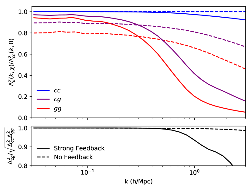
Figure 2: (Top) Ratio of CDM, gas and cross power spectra of the simulations with strong feedback to the CDM power spectrum without feedback. The gas power is cutoff on small scales due to its hydrodynamical pressure which is absent for CDM. Strong feedback reduces clustering in both the gas and CDM. (Bottom) The cross-correlation coefficient between gas and CDM. Strong feedback causes the gas to diverge from the CDM on small scales.

2.2 Velocity Fields

Computing velocity fields from a set of discrete particles is a known numerical challenge. The simulation momentum field can always be robustly estimated via the CIC interpolation technique, however, defining the velocity field as the ratio of the momentum to density fields is not well defined in cells with no particles. To our knowledge, the best way to compute velocity fields is the phase space projection method performed in Hahn et al. (2015) which was shown to perform better on small scales than other common schemes such as Delauney tessellation. The downside of utilizing the phase space structure of CDM is that it requires the ability to trace particles back to their initial conditions which requires extra memory and computational time. Another robust option is the “N-Nearest-Particles” method (NNP) which defines the velocity of a grid cell as the average of the N nearest particles to the grid cell. The 1NP method has been studied theoretically and numerically in Zhang et al. (2015); Zheng et al. (2015) and higher N has been used in Inman et al. (2015) to average over the random thermal velocities present in neutrino particles. While this technique is helpful in estimating velocities in low density regions, it has the downside that it does not use all particle information in high density regions.

Fortunately for us, we are using a rather coarse grid and the particle number density (64 particles per cubic grid cell) is very high. We can therefore get away with the use of CIC interpolation, setting any empty cells to zero. On lower resolution simulations with $512^{3}$ particles, we have checked that CIC gives comparable results to 8NP. We do not correct the velocity modes amplitude in Fourier space to remove the convolution with the CIC kernel function, as its functional form is not trivial when computing the velocity as the ratio of the momentum over the density. In order to verify that the CIC mass assignment scheme does not introduce numerical artifacts, we have computed the velocity field of the gas using the SPH radii of the particles (see e.g. Villaescusa-Navarro et al. (2014)). The velocity power spectrum of the gas was almost identical with both methods, demonstrating that our results are robust against these choices.

We show the CDM, gas, and relative velocity power spectra in Fig. 3, where the velocity power spectrum is defined as $\Delta^{2}_{v_{x}}+\Delta^{2}_{v_{y}}+\Delta^{2}_{v_{z}}$. We see that the CDM velocity power spectra are more or less the same in the two simulations whereas the gas power spectrum is significantly suppressed via feedback. This can be seen directly in the second column of Fig. 1 where relative motions extend to much larger scales when feedback is turned on. This difference leads to the large relative velocity power spectrum with feedback. We note that there is a bump in all the velocity power spectra at high $k\gtrsim 1.35h^{-1}{\rm Mpc}$ (most notably in the gas spectra with feedback). This does not seem to occur in the power spectra computed by Hahn et al. (2015) so we suspect it may be artificial and likely due to Poisson fluctuations.

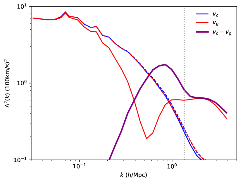
Figure 3: CDM (blue), gas (red), and relative (purple) velocity power spectra. Dashed curves have no feedback whereas solid curves have strong feedback. The suppression in the gas velocity power compared to CDM one on nonlinear scales leads to bulk relative motions. We suspect that features on scales smaller than the dotted vertical line (i.e. $k\gtrsim 1.35~{}h^{-1}$Mpc) are artificial.

To give a feel for the typical numbers involved, we compute the variance of the velocity fields, $\sigma_{i}^{2}=\int\Delta^{2}_{i}(k)d\ln(k)$. In order to not be sensitive to the artificial upturn in the velocity power, we only integrate to a maximum wavenumber of $1.35~{}h^{-1}{\rm Mpc}$. We show our results as a function of redshift in Fig. 4 as the purple curves. The feedback induced relative velocity peaks around redshift $1$ and is always significantly enhanced relative to the simulation without feedback. We see that their is a decrement in gas velocity leading to an increase in relative motions due to feedback.

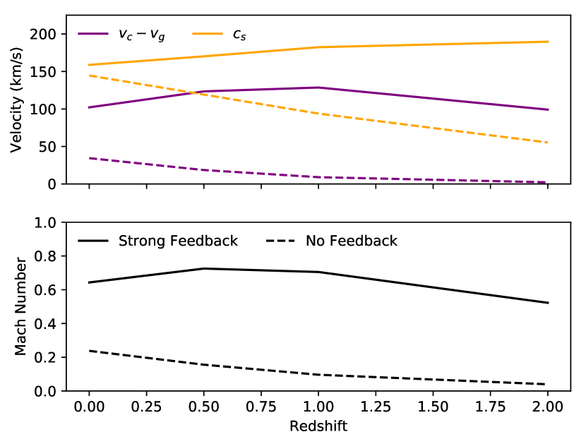
Figure 4: (Top) The variance of the relative velocity (purple) and gas sound speed (orange) as a function of redshift. Strong feedback (solid) increases both quantities significantly relative to no feedback (dashed). (Bottom) The Mach number, defined as the ratio of the relative velocity to the sound speed.

2.3 Sound Speed

Our next goal is to estimate the typical size of the gas sound speed to determine whether relative motions are supersonic or subsonic. Each SPH particle has an associated internal energy parameter, $u$. We interpolate the energy to a grid using CIC interpolation, consistent with our previous calculations. The sound speed is then calculated in each cell via $c_{s}=\sqrt{\gamma(\gamma-1)u}$ where $\gamma=5/3$ is the ratio of specific heats for a monatomic gas. Slices of sound speed are shown in the third column of Fig. 1. It clearly shares similar features to the relative velocity, but is not quite the same, leading to flows with different Mach numbers. We compute the variance of the internal energy and take $\sigma_{c_{s}}=\sqrt{\gamma(\gamma-1)\sigma_{u}}$. This result is shown in the top panel of Fig. 4 as solid (strong feedback) and dashed (no feedback) orange curves. The sound speed is always greater than the relative velocity. Thus, we expect on average there to be predominantly subsonic flows with typical Mach numbers shown in the bottom panel of Fig. 4. Nonetheless, we do still see regions of supersonic flows in the rightmost panels of Fig. 1.

3 Consequences for Large Scale Structure

3.1 Dipole Correlation Function

A perturber, such as a CDM halo, moving through a gas will cause wakes to form downstream from its motion. These distortions are asymmetric and depend on the direction of the relative motion. They are therefore not captured by the standard two point correlation function which only contains information about the matter distribution in spherical shells. Instead, we can use a three point function, the “dipole correlation function” which quantifies how likely you are to find a subsequent perturbation in a particular direction.

We compute the monopole and dipole correlation functions as $\xi_{ij0}(r)=\langle\delta_{i}(\vec{x})\delta_{j}(\vec{x}+\vec{r})\rangle$ and $\xi_{ij1}(r)=\langle\delta_{i}(\vec{x})\delta_{j}(\vec{x}+\vec{r})\hat{v}_{\rm rel}^{\rm avg}(\vec{x},\vec{x}+\vec{r})\cdot\hat{r}\rangle$, where $\hat{v}^{\rm avg}$ is the (unit) average relative velocity at $\vec{x}$ and $\vec{x}+\vec{r}$, i.e. $\vec{v}^{\rm avg}(\vec{x},\vec{x}+\vec{r})=(1/2)(\vec{v}(\vec{x})+\vec{v}(\vec{x}+\vec{r}))$. The algorithm describing this computation is given in Inman et al. (2017). We show the CDM-gas monopole and dipole correlation functions in the top panel of Fig. 5. The monopole is essentially unchanged by feedback on large scales, but is slightly suppressed on the small ones. The dipole is the opposite: feedback enhances the dipole by a significant amount for $r\sim 10$ Mpc/h. We also see that strong feedback causes the dipole to extend to much larger scales. This makes sense: as we have seen, the gas is much less clustered with strong feedback. In the bottom panel of Fig. 5 we show the polarizability, the ratio of the dipole to the monopole. We find that it peaks on scales around a few Mpc/h. We note that there is significant redshift evolution of the dipole correlation function. For instance, at redshift $2$, the strong feedback $\xi_{ij1}$ is always an order of magnitude larger than the no feedback one, regardless of scale. On the other hand, at redshift $0$ they become much more comparable. This could be due to the small amount of relative motion in the no feedback simulation that is growing with scalefactor, in addition to increasing contamination from nonlinear gravitational evolution of the density fields.

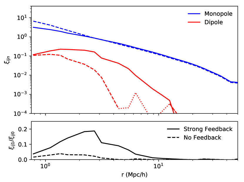
Figure 5: (Top) The monopole (blue) and dipole (red) correlation functions between cold dark matter and gas computed from simulations. Solid curves feature strong feedback whereas dashed curves have no feedback. The dotted red curve is the absolute value of the dipole with no feedback. The monopole is suppressed on small scales, whereas the dipole is enhanced on larger ones. (Bottom) The ratio between monopole and dipole for strong (solid) and no (dashed) feedback. Feedback enhances the polarizability of the IGM on scales of a few $h^{-1}{\rm Mpc}$.

3.2 Halo Dynamics

The large bulk motions induced by feedback should change the coordinates and velocities of halos relative to the no feedback simulation. By comparing the same halos between simulations, we can therefore estimate the net displacement and deceleration. The most robust way to match halos between simulations is to check that they contain the same particles, as has been performed in Mummery et al. (2017). We instead opt for a simpler method to match halos by enforcing that they are sufficiently similar in mass and position. Halo $i$ in one simulation is considered matched to halo $j$ in the other if $|m_{i}-m_{j}|/\sqrt{m_{i}m_{j}}\leq 0.5$ and $|\vec{r}_{i}-\vec{r}_{j}|\leq\ 0.5~{}\mbox{Mpc}/\mbox{h}.$ In the event that several halos satisfy these criteria, we select the closest one. We then repeat this procedure but swapping the simulations. We only consider halos that match each other and have masses greater than $5\times 10^{11}M_{\odot}$ corresponding to $\sim 1000$ or more CDM particles. In total, we match over $80\%$ of halos. In order to confirm the robustness of our method we have paired a fraction of the total halos by matching the IDs of their belonging particles. We find that the two methods produce very similar results.

Given matched halos, we then compute the difference in their positions and velocities, $\delta\vec{x}=\vec{x}(\chi)-\vec{x}(0)$ and $\delta\vec{v}=\vec{v}(\chi)-\vec{v}(0)$, where $\chi$ and 0 stand for the simulations with and without feedback, respectively. Between the simulations, we expect intrinsic differences in these quantities that are not directly due to the relative velocity external to the halos (e.g. the change in star formation, the change in halo mass and correspondingly different gravitational accelerations). To isolate dynamics due to larger scale flows, we need an estimate of the relative velocity. Rather than use the grid velocity fields, which would necessarily introduce anisotropies, we estimate the gas and CDM velocities in spheres of radius $5\ \mbox{Mpc}/\mbox{h}$ around each halo. Specifically, we compute the mean CDM velocity from all CDM particles and the mean internal energy and gas velocity from all SPH particles within the sphere. We then obtain $\vec{v}_{r}=\vec{v}_{c}-\vec{v}_{g}$ for all halos and define $\delta\vec{v}_{r}=\vec{v}_{r}(\chi)-\vec{v}_{r}(0)$.

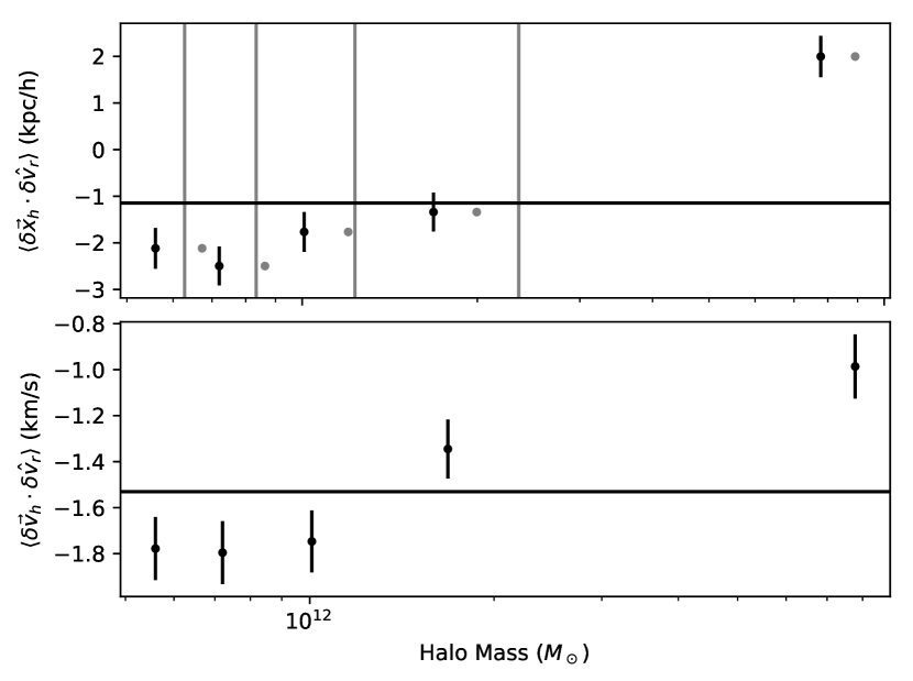
Figure 6: The change in halo positions (top) and velocities (bottom) in the direction of the relative velocity as a function of halo mass ($M\gtrsim 5\times 10^{11}M_{\odot}$) in the strong feedback simulation. The top panel also shows the mass bins as vertical lines and indicates the no feedback halo mass by grey points. Horizontal lines show the mean value of all halos considered. Potential causes for the acceleration include dynamical friction, Ram pressure, and gravitational infall while the mass dependence may be affected by halo environment.

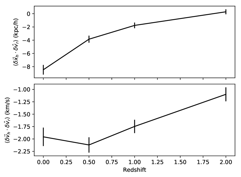
Figure 7: The mean change in halo positions (top) and velocities (bottom) in the direction of the relative velocity as a function of redshift. We include only halos with masses around $10^{12}M_{\odot}$ in this computation.

We next estimate the change in halo positions and velocities in the direction of the relative velocity; $\langle\delta\vec{x}\cdot\delta\hat{v}_{r}\rangle$ and $\langle\delta\vec{v}\cdot\delta\hat{v}_{r}\rangle$, respectively. We show the results as a function of mass in Fig. 6. We find that smaller halos tend to be displaced/decelerated further in the direction of the relative velocity than larger ones. Indeed we find that larger halos tend to move in the opposite direction (i.e. into the flow rather than with the flow) compared to smaller ones. We then select the third bin, corresponding to halo masses around $\sim 10^{12}M_{\odot}$ and show the results as a function of redshift in Fig. 7. Note that the errors in both figures are the errors on the mean, not the variance. This is only a part of the intrinsic variation in halo coordinates between simulations ( $\sqrt{\langle\delta\vec{x}^{2}\rangle}\sim\mathcal{O}(100\ \mbox{kpc}/\mbox{h}{})$ and $\sqrt{\langle\delta\vec{v}^{2}\rangle}\sim\mathcal{O}(20\ {\rm km}/{\rm s})$).

There are a number of potential mechanisms that can contribute to these accelerations. A hydrodynamic explanation is that gas flowing over the halo can push the gas in the halo via Ram pressure (Gunn & Gott, 1972). Alternatively, it could be entirely gravitational in nature. The gas flowing over a halo should be focused into a downstream wake via dynamical friction, which then pulls on the halo. We note that it is theoretically expected that uniform subsonic flows should not accelerate an isolated point-like halo (Ostriker, 1999). We discuss this prediction further in Appendix A and conclude that it is unlikely to hold in the cosmic web. Both Ram pressure and dynamical friction will yield negative values of $\langle\delta\vec{x}_{h}\cdot\delta\hat{v}_{r}\rangle$ and $\langle\delta\vec{v}_{h}\cdot\delta\hat{v}_{r}\rangle$. On the other hand, if the gas flows towards halos, but not over them, then there is just mutual gravitational infall, which will contribute the opposite sign. There are as well potential systematic effects. For instance, we do not consider the magnitude (and whether it depends on halo mass) of the gas velocity in our computations, instead using only $\delta\hat{v}_{r}$. The halo winds we use only conserve momentum statistically, not per event, and so some dynamics may be lost there. Furthermore, the amount of gas expelled from a halo and flowing over it may depend on the halo mass itself. Lastly, even the no feedback simulation has some regions with large relative velocities (see Fig. 1) and moreover has systematically heavier halos which can complicate the interpretation of the mass dependence. In practice, we expect a combination of effects to be occurring. We discuss some of our efforts at disentangling them in Appendix B.

4 Connection to Observables

4.1 The CDM Velocity

Determining halo peculiar velocities from LSS observations is notoriously tricky. One way is to simply estimate it from linear theory: $\vec{v}_{L}\propto-i\frac{\vec{k}}{k^{2}}\delta_{m}$. Since $\delta_{m}$ is not directly observable, the galaxy density field, $\delta_{g}$, is used instead. While the initial measurement of galaxy coordinates can be quite precise, the can be difficult to use as it is only a biased tracer of $\delta_{m}$. Furthermore, the linear velocity estimate is only accurate on sufficiently large scales. Lastly, we note that on sufficiently large scales both the gas and CDM have the same linear velocity. However, the inferred linear velocity field is not directly sensitive to feedback, so we can extract the relative velocity provided we have a direct measurement of the actual nonlinear gas velocity. An alternative approach is to measure the peculiar velocities directly, which requires both a distance and a redshift and is applicable only for low redshift galaxies (Hudson & Turnbull, 2012).

One way to mitigate nonlinearities is through reconstruction techniques which attempt to partially undo nonlinear gravitational evolution. These techniques work in Lagrangian space where the relevant quantity is the displacement field rather than the density field. The standard reconstruction procedure (Eisenstein et al., 2007) assumes the linear velocity field which we wish to obtain, so that may not be useful. However, there are a number of nonlinear reconstruction methods (e.g. Zhu et al. (2017); Schmittfull et al. (2017); Modi et al. (2018); Hada & Eisenstein (2018); Shi et al. (2018)) which use alternate methods to determine the displacement field. Utilizing these methods increases the available information (Pan et al., 2017) and has enabled better measurements of the baryon acoustic oscillations (Wang et al., 2017). However, the success of reconstruction in the presence of gas and feedback has not yet been studied.

4.2 The Gas Velocity

In addition to traditional probes of the LSS such as the positions and velocities of biased tracers, we may also consider the effects of relative motions on the Sunyaev-Zel’dovich effects (SZEs). The thermal SZE is caused by the upscattering of photons by an ionized gas in the Universe and is proportional to the cluster pressure. These regions also emit X-rays which can be used to determine the local gas density (Adam et al., 2017). This is therefore directly related to the sound speed, $c_{s}^{2}=\delta P/\delta\rho\sim\bar{P}/\bar{\rho}$, of the gas around a halo. The kinetic SZE arises when the ionized gas scattering the photons has a net peculiar velocity. Thus, its measurement tells us the gas velocity around a halo. Another possibility is to made use of high-resolution X-ray spectroscopy to determine gas velocities (Guainazzi & Tashiro, 2018). These measurements can also be used to probe the gas velocity (inflows and outflows) our galaxies and halos. The relative velocity changes significantly more than the gas velocity with feedback and so its measurement may be more sensitive. This then requires $v_{c}$, which could be obtained via linear density reconstruction: $\vec{v}_{c}\sim\vec{v}_{L}$. We note that the simultaneous use of thermal and kinetic SZE alongside linear velocity fields has already been performed (Schaan et al., 2016; Planck Collaboration et al., 2016). Utilizing all three would require an excellent understanding of the galaxy bias, however.Lastly, it is possible that strong feedback such as the large relative velocities studied here could bias estimations of the kinetic SZE (Park et al., 2018).

Nonetheless, it is plausible to obtain estimates of (or quantities analogous to) $c_{s}$ and $v_{r}$ for individual halos. Using our results, we can make a theoretical prediction for what to expect. We estimate $c_{s}$, $\vec{v}_{g}$ and $\vec{v}_{c}$ by averaging all particles in a sphere of $5$ Mpc/h as described in §3.2. We then plot a phase diagram which we show in Fig. 8 where each point represents a halo. Unsurprisingly, there is a clear effect of strong feedback as there are significantly more halos with large sound speeds and velocities. This is also clearly shown in the projected histograms where there is clear separation between the simulations. Finally, we see that $v_{r}\lesssim c_{s}$, in line with Fig. 4 and theoretical predictions (Ostriker, 1999).

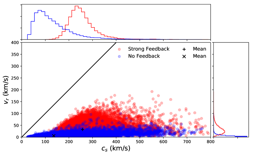
Figure 8: The relative velocity and sound speed computed in spherical shells of $5\ \mbox{Mpc}/\mbox{h}$ around each halo. Strong feedback enhances both quantities significantly. The top and right histograms project down to one variable. The diagonal line is $v_{r}=c_{s}$ to guide the eye.

5 Conclusion

We have studied some of the dynamical consequences associated with feedback induced relative velocity between the IGM and CDM. It is worth keeping in mind a few things, however. Firstly, we greatly amplified the strength of supernova kinetic feedback, such that we achieved winds of 1000s km/s. This was done to mimic some of the more energetic effects seen when AGN feedback is included (see, e.g., figures from the Illustris (Vogelsberger et al., 2014a; Pillepich et al., 2018) or Eagle (Schaye et al., 2015) simulations for striking examples) and to study the dependence of our results on the feedback efficiency. Secondly, we have not spent much time discussing what happens if feedback is low. Here, the details of gas bias matter significantly, and will likely be swamped by changes in the feedback model. Dealing with these considerations will require a more sophisticated feedback implementation, but in principle, do not hinder our results. A clear next step is to see to what extent the effects presented here are present in more realistic simulations.

It is also worth considering what other effects may mimic or contaminate our results. One (practically) guaranteed background is from cosmic neutrinos, which will also have a relative velocity Zhu et al. (2014); Inman et al. (2015); Inman et al. (2017) and dynamical friction Okoli et al. (2017), although of course no SZE. The numbers we obtain may be compared to the prediction for neutrino dynamical friction of Okoli et al. (2017) who found values of order $0.2\ {\rm km}/{\rm s}$ and $1.5\ \mbox{kpc}/\mbox{h}$ (depending on halo and neutrino properties) when averaged over $16$ Mpc/h. Of course, the key differences are that neutrinos are collisionless and therefore not subject to hydrodynamic forces, but more importantly that the baryons can contribute significantly more to the matter density since $\Omega_{g}\gg\Omega_{\nu}$. We therefore find that the IGM dipole signal could be a significant contaminant to the neutrino one, although it should not extend over as large of scales and the relative velocities may be in different directions. On the other hand, if there is a warm component to the dark matter it could also contribute and could be much more similar to gas. On smaller scales (i.e. $1$ Mpc/h or cluster sized scales), other effects come into play. The motions of galaxies through the halo can yield gravitational wakes behind the galaxy in the direction of the relative motion (Furlanetto & Loeb, 2002). Furthermore, galaxies themselves will feel Ram pressure (Gunn & Gott, 1972) due to the intracluster medium. This should lead to a galaxy-gas dipolar effects which could be enhanced if the ram pressure can strip gas from the galaxy (Abadi et al., 1999).

Finally, we re-emphasize that we have not considered more technical challenges, such as the understanding of galaxy bias, the relationship between galaxies and halos, and the computations of $v_{r}$ and $c_{s}$ from SZE measurements and galaxy surveys. Certainly, more study is required in this area.

Appendix A Dynamical friction in the expanding universe

An intriguing theoretical question is whether dynamical friction even exists for a gaseous medium. Ostriker (1999) computed the force a point perturber feels and found that, in the steady state limit, it is exactly zero for a gas in subsonic motion, but nonzero for a collisionless species of particles. Even if the steady state limit is not achieved, a perturber that is turned on at some time will feel a greatly reduced force when travelling subsonically. This is because the gas will try to produce a “front-back symmetry,” cancelling the drag force. In this appendix, we will consider what happens when this process occurs for fluids in an expanding Universe filled with large scale structure.

The equation of motion for a fluid is given by:

$$\ddot{\delta}_{g}+w^{2}(a)\delta_{g}=\frac{3}{2}H_{0}^{2}\Omega_{m}\delta_{m}a$$

where the frequency is given by $w(a)=akc_{s}(a)$ with $a$ being the scalefactor and $k$ the comoving wavenumber. In this equation, over-dots refer to the Newtonian time, s, which is related to the physical time, $t$, and conformal time, $\tau$, via $dt=ad\tau=a^{2}ds$. For slowly varying sound speeds, we can employ the WKB approximation and find the integral solution:

$$\delta_{g}(\tau,k)= G(s,s_{i})\dot{\delta}_{g}(\tau_{i})-\dot{G}(s,s_{i})\delta_{g}(\tau_{i})$$

$$+\frac{3}{2}H_{0}^{2}\Omega_{m}\int_{\tau_{i}}^{\tau}d\tau^{\prime}\delta_{m}(\tau^{\prime},k)(s-s^{\prime})\frac{G(s,s^{\prime})}{(s-s^{\prime})}$$ (1)

where the Green’s function $G(s,s^{\prime})$ is given by:

$$\frac{G(s,s^{\prime})}{(s-s^{\prime})}=\frac{\sin\left(\int_{s^{\prime}}^{s}ds^{\prime\prime}w(s^{\prime\prime})\right)}{(s-s^{\prime})\sqrt{w(s)w(s^{\prime})}}$$

and we have factored out the $s-s^{\prime}$ piece such that in the limit of $c_{s}\rightarrow 0$ that $G/(s-s^{\prime})\rightarrow 1$. The other two terms in Eq. A arise due to the non-homogeneous boundary conditions when $\tau_{i}$ is not $0$. We will always take $\tau_{i}=0$ and so these terms are not present. Eq. A is exact for a gas with constant frequency ($c_{s}(a)=c_{s}/a$) where $G(s,s^{\prime})/(s-s^{\prime})=j_{0}(kc_{s}(s-s^{\prime}))$. We will assume $c_{s}(a)=c_{s}/a$ throughout this Appendix.

Eq. A also applies to collisionless particles with a given distribution function $f(v)$, provided initial conditions are negligible and we use the appropriate Green’s function:

$$\frac{G(s-s^{\prime})}{(s-s^{\prime})}=\frac{\int dvv^{2}f(v)j_{0}(kv(s-s^{\prime}))}{\int dvv^{2}f(v)}.$$

For the Maxwell-Boltzmann distribution (MBd), $f(v)\propto\exp[-v^{2}/\sigma^{2}]$, and this integral can be done analytically to obtain:

$$\frac{G(s-s^{\prime})}{(s-s^{\prime})}=\exp\left[-\frac{\left(k\sigma(s-s^{\prime})\right)^{2}}{4}\right].$$

Because collisionless particles are dispersive (Inman & Pen, 2017), there is no value of $\sigma$ that matches $c_{s}$ at all scales. The closest definition to use is the small scale sound speed:

$$c_{s}^{2}=\frac{\int dvv^{2}f(v)}{\int dvf(v)}$$

which is equal to $\sigma^{2}/2$ for the MBd.

To include the effects of a bulk flow we can use Moving Background Perturbation theory (Tseliakhovich & Hirata, 2010). A constant, uniform bulk flow causes a comoving displacement, $\vec{d}(\tau,\tau^{\prime})=\int_{\tau^{\prime}}^{\tau}\vec{v}_{\rm rel}(\tau^{\prime\prime})d\tau^{\prime\prime}$, between the CDM and gas which becomes a phase in Fourier space $\delta_{c}(k)\rightarrow\delta_{c}(k)\exp[i\vec{k}\cdot\vec{d}]$ (Inman et al., 2017). To extract multipole moments, we can expand the phase:

$$\exp\left[i\vec{k}\cdot\vec{d}\right]=j_{0}(kd)+3i\mu j_{1}(kd)+...$$

The terms independent of $\mu$ constitute the monopole and terms proportional to $\mu$ the dipole. We can also expand the density contrast into multipoles as well $\delta=\delta_{0}+i\mu\delta_{1}+...$.

To proceed further, we will work in matter domination and assume that the gas or collisionless particles contribute negligibly to the matter density: $\delta_{m}\rightarrow\delta_{m}\exp[i\mu kd]$. In matter domination we have $H_{0}=2/\tau_{0}$, $\Omega_{m}=1$, $\delta_{m}(\tau,k)=a(\tau)\delta_{m}(1,k)$, $a(\tau)=(\tau/\tau_{0})^{2}$ and $s-s^{\prime}=-\tau_{0}^{2}(1/\tau-1/\tau^{\prime})$. Finally we need to assume a model for the induced displacement, $d$. Since the sound speed is decaying like $c_{s}\propto 1/a$, the relative velocity should eventually decay due to Hubble friction or else the bulk flows will become infinitely supersonic. We will therefore parameterize $d=v_{\rm rel}(s-s^{\prime})=Mc_{s}(s-s^{\prime})$ where $M$ is the Mach number.

Using Eq. A, these approximations, and changing variables to $x=\tau^{\prime}/\tau$ yields the following for the monopole and dipole:

$$\frac{\delta_{0}(a,k)}{\delta_{m}(a,k)} =6\int_{0}^{1}x(1-x)V(\bar{k}(1-x)/x)j_{0}(M\bar{k}(1-x)/x)dx$$ (2)

$$\frac{\delta_{1}(a,k)}{\delta_{m}(a,k)} =6\int_{0}^{1}x(1-x)V(\bar{k}(1-x)/x)3j_{1}(M\bar{k}(1-x)/x)dx$$ (3)

where $\bar{k}=kc_{s}\tau_{0}/\sqrt{a(\tau)}$, and $V(x)=j_{0}(x)$ for gas or $\exp\left[-x^{2}/2\right]$ for collisionless particles with a MBd. Qualitatively, $V(x)\leq 1$ and so $\delta_{0}$ is never greater than the CDM solution, $\delta_{m}$. For the monopole in the subsonic limit, $M\ll 1$, $j_{0}(M\bar{k}(1-x)/x)\to 1$ and we expect the monopole to be unperturbed. In the supersonic limit, $j_{0}$ will oscillate rapidly and we expect $\delta_{0}$ to become suppressed. The dipole on the other hand is small (and proportional to $M$) in the subsonic limit $3j_{1}(M\bar{k}(1-x)/x)\to M\bar{k}(1-x)/x$. It should also be suppressed in the highly supersonic regime.

We can now see that the situation is very different in the cosmological fluid equations used above compared to that of Ostriker (1999). The sound speed experiences Hubble friction and decays like $1/a$. This implies that the Jean’s wavenumber, $k_{J}^{2}=(3/2)H_{0}^{2}\Omega_{m}a/(ac_{s}(a))$ is increasing to smaller and smaller scales. This is reflected in our equations: taking $a\to\infty$ implies $\bar{k}\to 0$ and $\delta_{0}\equiv\delta_{m}$ whereas $\delta_{1}\equiv 0$. Thus, there will be no dipole distortions (for linearized equations, anyways) in the infinitely far future, but this is not due to the “front-back” symmetry found in non-expanding fluids with a static perturber. Instead, it is because the hot fluids tend to the growing CDM solution.

There is, however, a limit that much more closely matches the results of Ostriker (1999). This limit is the “instantaneous” limit: $\ddot{\delta}_{g}\ll(kc_{s})^{2}\delta_{g}$. We can achieve this by letting $\bar{k}\rightarrow\infty$. To see the effects of this, it is easiest to change variables in Eqs. 2 and 3 to $y=\bar{k}(1-x)/x$ in which case we obtain:

$$\frac{\delta_{0}}{\delta_{m}} =\frac{6}{\bar{k}^{2}}\int_{0}^{\infty}dy\frac{y}{(1+y/\bar{k})^{4}}V(y)j_{0}(My)$$ (4)

$$\frac{\delta_{1}}{\delta_{m}} =\frac{6}{\bar{k}^{2}}\int_{0}^{\infty}dy\frac{y}{(1+y/\bar{k})^{4}}V(y)3j_{1}(My).$$ (5)

For $M=0$, the limiting behaviours for Eq. 4 is $6/\bar{k}^{2}$, which is precisely the Jeans, or free streaming, scale in matter domination: $\frac{k_{fs}}{k}=\frac{\sqrt{6}}{\bar{k}}$. Eq. 5 is exactly zero, as required. Clearly, if we take $\bar{k}\to\infty$ both $\delta_{0}$ and $\delta_{1}$ are zero for non-trivial sound speeds. However, we can understand their limiting behaviour relative to the unperturbed ($M=0$) monopole, i.e. $\lim_{\bar{k}\to\infty}\delta_{i}(M)/\delta_{0}(0)$ for $i=0,1$. We show the result in Fig. 9 for both gas and collisionless MBd particles. We find that the steady-state dipole is exactly zero for subsonic collisional flows, but non-zero for collisionless ones. It is always non-zero for supersonic flows. This mimics the result seen in Ostriker (1999): in the instantaneous subsonic limit, the sound horizon of gas is effectively infinite and there is no dipole. Since there is no dipole in this limit, there should also be no gravitational force to cause backreaction in the CDM. On the other hand, this is quite an artificial limit and for finite $\bar{k}$ there will still be a dipole in the subsonic case.

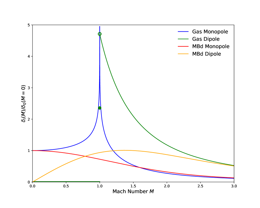
Figure 9: The instantaneous behaviour of the monopole and dipole relative to the zero relative velocity monopole as a function of Mach number. Blue and red curves correspond to a collisional gas whereas red and orange are a collisionless gas with a Maxwell-Boltzmann velocity distribution. Notably, the gas has no dipole for subsonic flows.

Appendix B Disentangling Halo Accelerators

The Ram pressure force scales like $\sim v^{2}$ (Gunn & Gott, 1972) whereas dynamical friction is expected to fall off like $\sim 1/v^{2}$ (Ostriker, 1999). We therefore expect $\delta\vec{v}\cdot\delta\hat{v}_{r}$ as a function of $\delta\hat{v}_{r}$ to be different for the two effects. We show this result in Fig. 10. While by eye the shape looks suggestive of dynamical friction, the mean value is very flat.

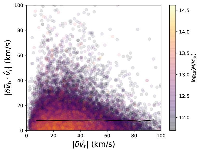
Figure 10: The differential acceleration of halos as a function of relative velocity. The black line shows the mean value.

Alternatively, we could see gravitational in-fall of gas into a halo. In this case we expect the halo to slightly move towards the gas, in the opposite direction of the dynamical friction case. To test this, we compute the dipole moment of the density: $\vec{d}\propto\sum(x_{i}-x_{h})$ where $x_{i}$ are the coordinates of particles within $5$ Mpc/h of a halo at $x_{h}$. We then define angles between the dipole and the relative velocity: $\cos\theta_{i}=\hat{d}_{i}\cdot\hat{v}_{r}$. We get two angles $i=c,g$ for each simulation. If dynamical friction is occurring, we expect the gas dipole to be anti-aligned with the relative velocity, whereas it will be aligned if it is gravitational in-fall. In order to remove contamination from bound gas in-falling with CDM, we compute $\cos\theta_{c}-\cos\theta_{g}$ and show the result in Fig. 11. The shift towards negative values is an indicator of in-fall.

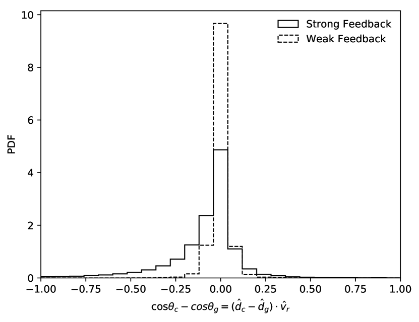
Figure 11: The alignment of the dipole and the relative velocity.

References

- Abadi et al. (1999) Abadi M. G., Moore B., Bower R. G., 1999, MNRAS, 308, 947
- Adam et al. (2017) Adam R., et al., 2017, A&A, 606, A64
- Dalla Vecchia & Schaye (2008) Dalla Vecchia C., Schaye J., 2008, MNRAS, 387, 1431
- Dubois et al. (2014) Dubois Y., et al., 2014, MNRAS, 444, 1453
- Eisenstein et al. (2007) Eisenstein D. J., Seo H.-J., Sirko E., Spergel D. N., 2007, ApJ, 664, 675
- Furlanetto & Loeb (2002) Furlanetto S. R., Loeb A., 2002, ApJ, 565, 854
- Guainazzi & Tashiro (2018) Guainazzi M., Tashiro M. S., 2018, preprint, (arXiv:1807.06903)
- Gunn & Gott (1972) Gunn J. E., Gott III J. R., 1972, ApJ, 176, 1
- Hada & Eisenstein (2018) Hada R., Eisenstein D. J., 2018, MNRAS, 478, 1866
- Hahn et al. (2015) Hahn O., Angulo R. E., Abel T., 2015, MNRAS, 454, 3920
- Haider et al. (2016) Haider M., Steinhauser D., Vogelsberger M., Genel S., Springel V., Torrey P., Hernquist L., 2016, MNRAS, 457, 3024
- Hudson & Turnbull (2012) Hudson M. J., Turnbull S. J., 2012, ApJ, 751, L30
- Hunter (2007) Hunter J. D., 2007, Computing in Science and Engineering, 9, 90
- Inman & Pen (2017) Inman D., Pen U.-L., 2017, Phys. Rev. D, 95, 063535
- Inman et al. (2015) Inman D., Emberson J. D., Pen U.-L., Farchi A., Yu H.-R., Harnois-Déraps J., 2015, Phys. Rev. D, 92, 023502
- Inman et al. (2017) Inman D., et al., 2017, Phys. Rev. D, 95, 083518
- Jing et al. (2006) Jing Y. P., Zhang P., Lin W. P., Gao L., Springel V., 2006, ApJ, 640, L119
- Lewis et al. (2000) Lewis A., Challinor A., Lasenby A., 2000, ApJ, 538, 473
- Loken et al. (2010) Loken C., et al., 2010, Journal of Physics: Conference Series, 256, 012026
- Modi et al. (2018) Modi C., Feng Y., Seljak U., 2018, J. Cosmology Astropart. Phys., 10, 028
- Mummery et al. (2017) Mummery B. O., McCarthy I. G., Bird S., Schaye J., 2017, MNRAS, 471, 227
- Okoli et al. (2017) Okoli C., Scrimgeour M. I., Afshordi N., Hudson M. J., 2017, MNRAS, 468, 2164
- Ostriker (1999) Ostriker E. C., 1999, ApJ, 513, 252
- Pan et al. (2017) Pan Q., Pen U.-L., Inman D., Yu H.-R., 2017, MNRAS, 469, 1968
- Park et al. (2018) Park H., Alvarez M. A., Bond J. R., 2018, ApJ, 853, 121
- Pillepich et al. (2018) Pillepich A., et al., 2018, MNRAS, 473, 4077
- Planck Collaboration et al. (2016) Planck Collaboration et al., 2016, A&A, 586, A140
- Planck Collaboration et al. (2018) Planck Collaboration et al., 2018, preprint, (arXiv:1807.06209)
- Rudd et al. (2008) Rudd D. H., Zentner A. R., Kravtsov A. V., 2008, ApJ, 672, 19
- Schaan et al. (2016) Schaan E., et al., 2016, Phys. Rev. D, 93, 082002
- Schaye et al. (2015) Schaye J., et al., 2015, MNRAS, 446, 521
- Schmidt (2016) Schmidt F., 2016, Phys. Rev. D, 94, 063508
- Schmittfull et al. (2017) Schmittfull M., Baldauf T., Zaldarriaga M., 2017, Phys. Rev. D, 96, 023505
- Shi et al. (2018) Shi Y., Cautun M., Li B., 2018, Phys. Rev. D, 97, 023505
- Springel (2005) Springel V., 2005, MNRAS, 364, 1105
- Springel & Hernquist (2003) Springel V., Hernquist L., 2003, MNRAS, 339, 289
- Springel et al. (2001) Springel V., Yoshida N., White S. D. M., 2001, New Astron., 6, 79
- Springel et al. (2017) Springel V., et al., 2017, preprint, (arXiv:1707.03397)
- Tornatore et al. (2010) Tornatore L., Borgani S., Viel M., Springel V., 2010, MNRAS, 402, 1911
- Tseliakhovich & Hirata (2010) Tseliakhovich D., Hirata C., 2010, Phys. Rev. D, 82, 083520
- Valkenburg & Villaescusa-Navarro (2017) Valkenburg W., Villaescusa-Navarro F., 2017, MNRAS, 467, 4401
- Villaescusa-Navarro et al. (2014) Villaescusa-Navarro F., Viel M., Datta K. K., Choudhury T. R., 2014, J. Cosmology Astropart. Phys., 9, 050
- Vogelsberger et al. (2014a) Vogelsberger M., et al., 2014a, MNRAS, 444, 1518
- Vogelsberger et al. (2014b) Vogelsberger M., et al., 2014b, Nature, 509, 177
- Wang et al. (2017) Wang X., Yu H.-R., Zhu H.-M., Yu Y., Pan Q., Pen U.-L., 2017, ApJ, 841, L29
- Zennaro et al. (2017) Zennaro M., Bel J., Villaescusa-Navarro F., Carbone C., Sefusatti E., Guzzo L., 2017, MNRAS, 466, 3244
- Zhang et al. (2015) Zhang P., Zheng Y., Jing Y., 2015, Phys. Rev. D, 91, 043522
- Zheng et al. (2015) Zheng Y., Zhang P., Jing Y., 2015, Phys. Rev. D, 91, 043523
- Zhu et al. (2014) Zhu H.-M., Pen U.-L., Chen X., Inman D., Yu Y., 2014, Physical Review Letters, 113, 131301
- Zhu et al. (2017) Zhu H.-M., Yu Y., Pen U.-L., Chen X., Yu H.-R., 2017, Phys. Rev. D, 96, 123502
- van der Walt et al. (2011) van der Walt S., Colbert S. C., Varoquaux G., 2011, Computing in Science and Engineering, 13, 22