Joint Latent Class Trees: A Tree-Based Approach to Modeling Time-to-event and Longitudinal Data

Abstract

In this paper, we propose a semiparametric, tree based joint latent class modeling approach (JLCT) to model the joint behavior of longitudinal and time-to-event data. Existing joint latent class modeling approaches are parametric and can suffer from high computational cost. The most common parametric approach, the joint latent class model (JLCM), further restricts analysis to using time-invariant covariates in modeling survival risks and latent class memberships. Instead, the proposed JLCT is fast to fit, and can use time-varying covariates in all of its modeling components. We demonstrate the prognostic value of using time-varying covariates, and therefore the advantage of JLCT over JLCM on simulated data. We further apply JLCT to the PAQUID data set and confirm its superior prediction performance and orders-of-magnitude speedup over JLCM.

Keywords: Biomarker; Conditional independence; Recursive partitioning; Survival data; Time-varying covariates.

1 Introduction

Clinical studies often collect three types of data on each patient: the time to the event of interest (possibly censored), the longitudinal measurements on a continuous response (for example, some sort of biomarker viewed as clinically important), and an additional set of covariates (possibly time-varying) about the patient. These studies then focus on analyzing the relationship between the time-to-event and the longitudinal responses, using the additional covariates. In particular, clinical studies are often interested in the idea of uncovering latent classes among the population of patients, which can be used to describe disease progression in clinical studies [1, 2, 3]. The idea of latent classes is partially motivated by the fact that many diseases have different stages; examples include dementia [4], AIDS [5], cancer [6], and chronic obstructive pulmonary disease (COPD) [7]. Once those stages are identified, one can design personalized medicine that, for a particular patient, changes with membership in different stages [8]. From this point of view, incorporating the time-varying nature of latent class membership into any modeling strategy is crucial, and any approach that does not allow for time-varying membership of latent classes cannot possibly be informative in the implementation of what is necessarily dynamic personalized medicine treatment. The desire to find latent classes in order to design personalized treatment also extends to other contexts as well.

Currently the clinical definitions of stages of a disease consist of using diagnostic findings (such as biomarkers) to produce clusters of patients. In this paper, we focus on an alternative approach to find data-dependent and possibly time-varying latent classes, which uncovers potentially meaningful stages by modeling the biomarker trajectories and survival experiences together. This is known as the joint latent class problem.

The joint latent class model (JLCM) [1, 9, 3, 10] is the most common approach for constructing latent classes that account for the joint behavior of time-to-event and longitudinal data. JLCM assumes that the population of patients consists of multiple latent classes, and models the latent class memberships by a multinomial logistic regression model. The key assumption of JLCM is that, conditioning on her latent class membership, a patient’s time-to-event and longitudinal responses are independent. JLCM further assumes that the latent classes are homogeneous and thus patients within a latent class follow the same survival and longitudinal model. The assumed latent classes could potentially represent clinically meaningful subpopulations, but such a connection requires further clinical research.

JLCM is a parametric approach, which estimates the parameters for all modeling components via maximizing the log-likelihood function. However, this can be prohibitively slow for large scale data. In addition, software implementations of JLCM [10] cannot use time-varying covariates in its latent class membership and survival models, which can greatly reduce its prediction performance. In Appendix A, we give a brief introduction to JLCM, and discuss at length its strengths and weaknesses; see also [11].

A nonparametric approach that addresses some of these issues would be desirable, and tree-based approaches [12, 13] are natural candidates. Tree-based methods are powerful modeling tools in statistics and data mining, especially because they are fast to construct, able to uncover nonlinear relationships between covariates, and intuitive and easy to explain. In this work, we propose the joint latent class tree (JLCT) method for the joint latent class problem, which consists of two steps. The first and primary step of JLCT is to provide a tree-based partitioning that uncovers meaningful latent classes of the population. JLCT, like JLCM, is based on the key assumption that conditioning on latent class membership, time-to-event and longitudinal responses are independent. JLCT therefore looks for a tree-based partitioning such that within each estimated latent class defined by a terminal node, the time-to-event and longitudinal responses display a lack of association. In the second step, we assign each observation to a latent class (i.e. terminal node of the constructed tree), and independently fit any type of survival and longitudinal models, using the class membership information. Since these time-to-event and longitudinal models can be fully parametric if desired, JLCT can be viewed as a semiparametric approach to the problem.

JLCT has two major advantages over JLCM. First, JLCT is computationally more favorable, for two reasons: (a) it is very efficient to fit a tree to uncover complex relationships between covariates, and (b) JLCT separates fitting the survival and longitudinal outcomes from uncovering the latent classes, whereas JLCM fits longitudinal, survival, and latent classes altogether. The second advantage lies in flexible modeling: JLCT addresses the time-invariant limitation of JLCM by using time-varying covariates as the splitting variables to construct the tree. Furthermore, once a tree is constructed, it is up to the user to decide which type of survival models and which covariates to use within each terminal node, depending on the analyst’s modeling choices and preferences. Both advantages are verified by our experimental results: JLCT is orders of magnitude faster, and it achieves better prediction performances than JLCM by adopting more flexible models.

The rest of the paper is organized as follows. In Section 2 we introduce the setup of the modeling problem, and describe our joint latent class tree (JLCT) method. In Section 3 we use simulations to compare JLCT with JLCM in terms of prediction performance and running time under various latent class scenarios. Finally, in Section 4 we apply JLCT to a real data set, and demonstrate that JLCT admits competitive (or superior) prediction performance, while being potentially orders of magnitude faster than both the JLCM and a popular alternative approach to joint modeling, the shared random effects model (SREM).

2 Constructing a tree to uncover conditional independence

2.1 Modeling setup

Assume there are $N$ subjects in the sample. For each subject $i$, we observe $n_{i}$ repeated measurements of a longitudinal outcome at times $\boldsymbol{t}_{i}=(t_{i1},\dots,t_{in_{i}})^{\prime}$. We denote the vector of longitudinal outcomes by $\boldsymbol{Y}_{i}=(y_{it_{i1}},\dots,y_{it_{in_{i}}})^{\prime}$. In addition, for each subject $i$, we observe a vector of covariates $\boldsymbol{X}_{it}$ at each measurement time $t\in\boldsymbol{t}_{i}$. These covariates can be either time-invariant or time-varying. Each subject is also associated with a time-to-event tuple $(T_{i},\delta_{i})$, where $T_{i}$ is the time of the event, and $\delta_{i}$ is the censor indicator with $\delta_{i}=0$ if subject $i$ is censored at $T_{i}$, and $\delta_{i}=1$ otherwise.

We assume there exist $G$ latent classes, and let $g_{it}\in\{1,\dots,G\}$ denote the latent class membership of subject $i$ at time $t$. Let $\boldsymbol{g}_{i}=(\boldsymbol{g}_{it_{i1}},\cdots,\boldsymbol{g}_{it_{in_{i}}})$ denote the vector of latent class memberships of subject $i$ at each measurement time $t\in\boldsymbol{t}_{i}$. We assume the latent class membership $g_{it}$ is determined by a subset of covariates $\boldsymbol{X}_{it}$, denoted by $\boldsymbol{X}^{\text{g}}_{it}$. The latent classes are assumed to be homogeneous, in the sense that the joint distribution of the longitudinal and time-to-event variables is the same for all observations within a latent class.

The joint latent class modeling problem proposed here makes the same key assumption as JLCM: a patient’s time-to-event $(T_{i},\delta_{i})$ and longitudinal outcomes $(\boldsymbol{Y}_{i})$ are independent conditioning on her latent class membership $(\boldsymbol{g}_{i})$. Unlike JLCM where the membership of a subject does not vary over time, JLCT allows the elements in $\boldsymbol{g}_{i}$ to change. Thus we need a slightly more involved definition of “conditional independence.” For subject $i$ and the time interval between any two consecutive observations, $I_{ik}=[t_{ik},t_{i(k+1)})$, conditioning on the event that subject $i$’s membership equals $g\in G$ on this interval $\big{(}\{g_{it}=g\mid t\in I_{ik}\}\big{)}$, the longitudinal process on the time interval $(y_{it}\mid t\in I_{ik})$ and the time-to-event outcome $(T_{i},\delta_{i})$ are independent. More precisely, for every subject $i$, every corresponding time interval $I_{ik}$, and every $g\in G$,

$$(T_{i},\delta_{i})\perp(y_{it}\mid t\in I_{ik})\text{, conditioning on the event }\{g_{it}=g\mid t\in I_{ik}\}.$$

The motivation for the conditional independence assumption in joint latent class modeling comes from the hypothesis that observed associations between the longitudinal and time-to-event variables over the entire population are spurious, being driven by heterogeneity in levels of the variables between latent classes. Without controlling the latent class membership $\boldsymbol{g}_{i}$, time-to-event and longitudinal outcomes may appear to be correlated because each is related to the latent class, but given $\boldsymbol{g}_{i}$ the two are independent of each other, and therefore the longitudinal outcomes have no prognostic value for time-to-event given the latent class.

Construction of the tree is based on working assumptions for the longitudinal and time-to-event processes (recall, however, that once tree-based latent classes are determined, the analyst is free to fit any models they wish to the observations in each estimated class). Conditioning on latent class membership, the working assumption is that the time-to-event tuple $(T_{i},\delta_{i})$ depends on a subset of covariates $\boldsymbol{X}^{\text{s}}_{it}$ observed at time $t\in\boldsymbol{t}_{i}$, through the extended Cox model for time-varying covariates [14]:

$$h_{i}(t|g_{it}=g)=h_{0g}(t)e^{\boldsymbol{X}^{\text{s}}_{it}{\boldsymbol{b}}_{g}},$$ (1)

where ${\boldsymbol{b}}_{g}$ is the vector of class-specific slope coefficients, and $h_{0g}$ the class-specific baseline hazard function. In Section 2.2, we show how to use this extended Cox model (1) to design the tree splitting criterion. In order to fit the extended Cox model (1) using the longitudinal outcome variable as a predictor, and perhaps other time-varying covariates, we need to convert the original data into left-truncated right-censored (LTRC) data, which is often referred to as a “counting process approach” [15, 16]. The conversion is described in detail in Appendix B.

The working assumption for the longitudinal outcomes is that they come from a linear mixed-effects model [17]:

$$y_{it}|_{g_{it}=g}=\boldsymbol{X}^{\text{f}}_{it}\boldsymbol{\beta}+\boldsymbol{X}^{\text{r}}_{it}\boldsymbol{u}_{g}+v_{i}+\varepsilon_{it},\quad\boldsymbol{u}_{g}\sim\mathcal{N}(0,\boldsymbol{\Sigma}_{r}),\quad v_{i}\sim\mathcal{N}(0,\sigma_{1}^{2}),\quad\varepsilon_{it}\sim\mathcal{N}(0,\sigma_{2}^{2}).$$ (2)

where $\boldsymbol{X}^{\text{f}}_{it}$ and $\boldsymbol{X}^{\text{r}}_{it}$ are the subsets of covariates associated with a fixed effect vector $\boldsymbol{\beta}$ and a latent class-specific random effect vector $\boldsymbol{u}_{g}$, respectively. The random effect vector $\boldsymbol{u}_{g}$ is independent across latent classes $g=1,\dots,G$, the subject-specific random intercept $v_{i}$ is independent across subjects and independent of the random effects $\boldsymbol{u}_{g}$, and the error $\varepsilon_{it}$ is independent and normally distributed with mean $0$ and variance $\sigma_{2}^{2}$, and independent of all of the random effects. To reduce model complexity, we only use a random intercept for each subject $i$ here, but in principle we can include any random effects on the subject level. Model selection for predicting longitudinal outcomes does not affect the construction of JLCT tree and is beyond the scope of this paper.

We have introduced four subsets of covariates so far: $\boldsymbol{X}^{\text{g}}_{it}$ for the latent classes, $\boldsymbol{X}^{\text{f}}_{it}$ for the fixed effects, $\boldsymbol{X}^{\text{r}}_{it}$ for the random effects, and $\boldsymbol{X}^{\text{s}}_{it}$ for the time-to-event. Each of the four subsets can contain time-varying covariates, and the four subsets can be either identical, or share common covariates, or share no covariates at all.

2.2 Joint Latent Class Tree (JLCT) methodology

In this section we formally introduce JLCT, the joint latent class tree approach. As discussed in the introduction, JLCT consists of two steps: the first and primary step is to construct a tree-based partitioning of the population; in the second step, JLCT independently fits survival and longitudinal models, using the proposed latent class memberships from the first step.

Step 1: Construct a tree-based partitioning.

Since the joint latent class model assumes conditional independence within each latent class, JLCT looks for a tree-based partitioning such that within each estimated class defined by a terminal node, the time-to-event and longitudinal outcomes display a lack of association. JLCT recursively splits a node into two children nodes according to a splitting criterion until some stopping criteria are met. The splitting criterion ensures that the two children nodes are more “homogeneous” than their parent node, where the notion of “homogeneous” is measured by how apparently independent the two variables are conditioning on the node.

Specifically, the splitting criterion repeatedly uses the test statistic for the hypothesis test

$$H_{0}:b_{y}=0,\quad\text{vs.}\quad H_{1}:b_{y}\neq 0,$$ (3)

under the extended Cox model

$$h(t,\boldsymbol{X}^{\text{s}}_{i},\boldsymbol{Y}_{i})=h_{0}(t)e^{y_{it}b_{y}+\boldsymbol{X}^{\text{s}}_{it}{\boldsymbol{b}}_{x}},$$ (4)

which is fitted using all the data within the node to split. Thus, the null hypothesis ($b_{y}=0$) corresponds to the longitudinal outcome having no relationship with the time-to-event in the node. We use the log-likelihood ratio test (LRT) for the hypothesis test (3) in all experiments; simulations indicate that the Wald test gives similar results. Note that the time-to-event formulation (4) is only being used as a splitting criterion, not as a representation of the true relationship between $\boldsymbol{Y}_{i}$ and $(T_{i},\delta_{i})$.

We will denote the test statistic of the hypothesis test (3) as TS. The smaller the value of TS is, the less related longitudinal outcomes $\boldsymbol{Y}_{i}$ are to the time-to-event data $(L_{it},R_{it},\delta_{it})$ within the current node. JLCT seeks to partition observations using covariates in $\boldsymbol{X}^{\text{g}}$, such that TS is small within each leaf node, until TS is less than a specified stopping parameter $s$. More formally, the tree splitting procedure works as follows:

1. At the current node, compute the test statistic TS${}_{\text{parent}}$.

2. If TS${}_{\text{parent}}<s$, stop splitting. Otherwise proceed.

3. For every split variable $X_{j}\in\boldsymbol{X}^{\text{g}}$, and possible split point $C$,

   1. Define two children nodes

      $$R_{\text{left}}(j,C)=\{(i,t):x_{itj}\leq C\},\quad R_{\text{right}}(j,C)=\{(i,t):x_{itj}>C\}.$$

   2. Ignore this split if either node violates the restrictions specified in the control parameters. (Details are given near the end of this section.) Otherwise proceed.

   3. At each child node, determine the test statistics TS${}_{\text{left}}(j,C)$, TS${}_{\text{right}}(j,C)$ respectively.

   4. Compute the score $S(j,C)=\texttt{TS}_{\text{parent}}-\texttt{TS}_{\text{left}}(j,C)-\texttt{TS}_{\text{right}}(j,C)$.

4. Scan through all pairs of $(j,C)$ to find $(j^{*},C^{*})=\operatorname*{arg\,max}_{j,C}S(j,C)$, and split the current node on variable $j^{*}$ at split point $C^{*}$.

JLCT recursively splits nodes according to the above procedure, until none of the terminal nodes can be further split. Under the null model $H_{0}$ in (3), the distribution of TS is approximately a $\chi^{2}_{1}$ distribution. By default, we adopt the stopping criterion $\texttt{TS}_{\text{parent}}<3.84$, which corresponds to the 5% tail of the $\chi^{2}_{1}$ distribution. We have also explored alternative stopping criteria $\texttt{TS}_{\text{parent}}<2.71$ and $\texttt{TS}_{\text{parent}}<6.63$, which corresponds to the 10% and 1% tail of the $\chi^{2}_{1}$ distribution, respectively, and find that these three stopping criteria have very similar performance in both simulations (Section 3.5) and the PAQUID dataset (Section 4.3). Note that this hypothesis test-based stopping criterion is similar in spirit (although different in purpose) to the approach used in conditional inference trees [18], as opposed to the greedy overfit-and-prune-back strategy of CART-type trees.

Standard control parameters for trees, such as the minimal number of observations in any terminal node, the minimal improvement in the “purity” by a split, etc., also apply to the JLCT method. In addition, we introduce two control parameters that are specific to JLCT:

• Minimum number of events in any terminal node. This parameter ensures that the survival model in each terminal node is fit on meaningful survival data with enough occurrences of events (that is, uncensored observations). By default, this parameter is set to the number of covariates used for the Cox PH model.

• Upper bound on the variance of the estimated coefficients in all survival models at tree nodes. This parameter ensures that the fitted coefficients of the survival models are numerically stable. By default this parameter is set to $10^{5}$.

These two new control parameters enforce reliability of the fitted survival models at all nodes, which further produces reliable test statistics to reflect the relationships between the time-to-event and the longitudinal outcomes.

Step 2: Fit survival and longitudinal models.

Once the tree is constructed, we view each terminal node as an estimated latent class, and obtain the “predicted” latent class membership $\hat{g}_{it}$ for each subject $i$ at time $t$. We then fit the following two models separately:

• Fit a survival model to time-to-event data $(T_{i},\delta_{i})$, using input covariates $\boldsymbol{X}^{\text{s}}_{it}$ and the predicted latent class membership $\hat{g}_{it}$.

• Fit a longitudinal model to longitudinal outcomes $y_{it}$, using input covariates $\boldsymbol{X}^{\text{f}}_{it}$, $\boldsymbol{X}^{\text{r}}_{it}$, and the predicted latent class membership $\hat{g}_{it}$.

By default, we use the extended Cox model (1) for the survival data, and the linear mixed-effects model (2) for the longitudinal data, but the user is free to make any modeling choices they wish.

3 Simulation results

In this section, we use simulations to study the behavior of JLCT, and compare JLCT with JLCM. We mainly focus on the case where all of the covariates are time-varying, and provide more simulation results for the time-invariant case in Appendix C. We demonstrate via these simulations that JLCT is a competitive alternative to JLCM for the following reasons:

1. It provides more accurate predictions. JLCT significantly outperforms JLCM in terms of survival and longitudinal prediction accuracies. We further show that the advantage comes primarily from using time-varying predictors.

2. It is more effective at uncovering true latent classes. In the simulations JLCT is highly effective at identifying the true latent classes when the latent structure is consistent with the form of a tree. Further, under the null scenario where there are no latent classes, JLCT almost always makes the correct decision of making no splits.

3. It is orders of magnitude faster. JLCT provides effective prediction and latent class identification while also being orders of magnitude faster to fit, due to its use of a fast tree algorithm to identify latent classes.

3.1 Data

We simulate five randomly distributed, time-varying covariates $X_{1},\cdots,X_{5}$, and use them to generate latent class memberships, time-to-event, and longitudinal outcomes. The data are generated such that the time-to-event is correlated with the longitudinal outcomes, but the two are independent conditioning on the latent classes. Thus, the key assumption of conditional independence holds on the simulated data. We consider various data generating schemes along two directions:

1. The structure of latent classes. We consider four ways of generating latent classes (as functions of covariates $X_{1}$ and $X_{2}$): tree partition, linear separation, non-linear separation, and asymmetric tree partition, which are shown in Figure 1. Class membership for a subject at any time $t$ is randomly drawn with probability $p_{0}$ being the class determined by $X_{1t}$ and $X_{2t}$, and $1-p_{0}$ being any of the remaining three classes. When $p_{0}=1$, the latent class membership corresponds to a deterministic partitioning based on $X_{1t},X_{2t}$; on the other hand, when $p_{0}=0.25$, the latent class membership is randomly determined and independent of $X_{1t},X_{2t}$. In addition, we include the null scenario where there are no latent classes. The value of $p_{0}$ does not matter here, and we set $p_{0}$ to 1 only as a placeholder.

2. The distribution of time-to-event data. We consider three distributions for baseline hazards of time-to-event data: exponential, Weibull with decreasing hazards with time (Weibull-D), and Weibull with increasing hazards with time (Weibull-I). We also consider various censoring rates: no censoring, light censoring, and heavy censoring, where approximately 0%, 20%, and 50% observations are censored, respectively.

We give a full description of the simulation setup in Appendix D, as well as a simpler setup with time-invariant covariates in Appendix C.

(a) Tree

(b) Linear

(c) Nonlinear

(d) Asymmetric

Figure 1: Four structures of latent class membership based on $X_{1}$ and $X_{2}$: (a) Tree partition, (b) Linear partition, (c) Nonlinear partition, (d) Asymmetric tree partition.

3.2 Models

Given the simulated data, JLCT uses $\boldsymbol{X}^{\text{s}}=\{X_{3},X_{4},X_{5}\}$ to model time-to-event data, $\boldsymbol{X}^{\text{f}}=\boldsymbol{X}^{\text{r}}=\{X_{1},\dots,X_{5}\}$ to model fixed and random effects for longitudinal outcomes, and ${\boldsymbol{X}^{\text{g}}}^{(\text{JLCT})}=\{X_{1},\dots,X_{5}\}$ to model latent class memberships. In order to match the maximum number of latent classes allowed for JLCM , all JLCT models are pruned to have no more than 6 terminal nodes. We fit the JLCT models using the jlctree function of our package jlctree (see Appendix H for more details). Note that this allows both methods to potentially uncover the true latent classes; clearly if the maximum number of classes allowed is smaller than the true number neither method can be very effective. Unlike for JLCM, the computing time for JLCT is not sensitive to the choice of the maximum number of terminal nodes, so if desired this number can be varied to provide a sensitivity analysis in the analysis of real data.

JLCM uses almost the same subsets of covariates as JLCT, except for latent classes. Since tree-based approaches automatically use interactions between covariates to partition the population, for fair comparison we include an additional interaction term in JLCM’s latent classes modeling: ${\boldsymbol{X}^{\text{g}}}^{(\text{JLCM})}=\{X_{1},\dots,X_{5},X_{1}X_{2}\}$. We allow class-specific coefficients and class-specific Weibull baseline risk functions for its survival model. The optimal number of latent classes is chosen from $\{2,3,4,5,6\}$ using BIC. We fit the JLCM models using the Jointlcmm function of the lcmm package [19].

We can directly fit JLCT to the simulated data where all covariates are time-varying. However, JLCM does not support time-varying covariates in either the latent class or the survival model. In the implementation of JLCM, i.e. the Jointlcmm function of the lcmm package, if a time-varying covariate is used in either model, by default Jointlcmm will take the first encountered value per subject as a baseline value and only use that. Thus, we can still fit JLCM with the simulated time-varying covariates, but JLCM automatically replaces $\boldsymbol{X}^{\text{s}},\boldsymbol{X}^{\text{g}}$ with ${\boldsymbol{X}^{\text{s}}}|_{\text{1st}},{\boldsymbol{X}^{\text{g}}}|_{\text{1st}}$, respectively, where ${X}|_{\text{1st}}$ denotes the first encountered value of a time-varying covariate $X$.

Since JLCM only uses the first encountered values per subject for covariates $\boldsymbol{X}^{\text{s}},\boldsymbol{X}^{\text{g}}$, it is not clear whether differences in performance of JLCM and JLCT are due to the additional information contained in later values of time-varying covariates, or because of the differences in the methodology itself. For the purpose of decomposing the difference, we also examine versions of JLCT that are restricted to using ${\boldsymbol{X}^{\text{s}}}|_{\text{1st}}$ and ${\boldsymbol{X}^{\text{g}}}|_{\text{1st}}$. Table 1 summarizes the various combinations of covariates we used to fit JLCT and JLCM models. Note that JLCM uses the same amount of information as JLCT₂, while JLCT₄ is the default JLCT method.

Table 1: Simulation: covariates used to fit JLCT and JLCM models

Model	Time-to-event	Latent class	Longitudinal
JLCT1	$\boldsymbol{X}^{\text{s}}$	no splitting	$\boldsymbol{X}^{\text{f}},\boldsymbol{X}^{\text{r}}$
JLCT2	${\boldsymbol{X}^{\text{s}}}|_{\text{1st}}$	${\boldsymbol{X}^{\text{g}}}|_{\text{1st}}^{(\text{JLCT})}$	$\boldsymbol{X}^{\text{f}},\boldsymbol{X}^{\text{r}}$
JLCT3	${\boldsymbol{X}^{\text{s}}}|_{\text{1st}}$	${\boldsymbol{X}^{\text{g}}}^{(\text{JLCT})}$	$\boldsymbol{X}^{\text{f}},\boldsymbol{X}^{\text{r}}$
JLCT4	$\boldsymbol{X}^{\text{s}}$	${\boldsymbol{X}^{\text{g}}}^{(\text{JLCT})}$	$\boldsymbol{X}^{\text{f}},\boldsymbol{X}^{\text{r}}$
JLCM	${\boldsymbol{X}^{\text{s}}}|_{\text{1st}}$	${\boldsymbol{X}^{\text{g}}}|_{\text{1st}}^{(\text{JLCM})}$	$\boldsymbol{X}^{\text{f}},\boldsymbol{X}^{\text{r}}$

3.3 Evaluation metrics

We use the following metrics to measure and compare model performances. To compute the out-of-sample measures, at each simulation run we generate a new random sample of $N$ subjects, using the same data generating process as for the in-sample data.

Time-to-event prediction

We use the integrated squared error (ISE) to measure the divergence between the true and the predicted survival curves. The ISE for a set of $N$ subjects is defined as

$$\text{ISE}=\frac{1}{N}\sum_{i=1}^{N}\frac{1}{\max_{i}T_{i}}\int_{0}^{\max_{j}T_{j}}\big{(}\hat{S}_{i}(t)-S_{i}(t)\big{)}^{2}dt,$$

where $\hat{S}_{i}(t)$ and $S_{i}(t)$ are the predicted and the true survival probability for subject $i$ at time $t$, respectively. We compute ISE on in-sample subjects (ISE${}_{\text{in}}$) and on out-of-sample subjects (ISE${}_{\text{out}}$). In order to predict survival probabilities beyond subject $i$’s event time $T_{i}$, we assume that covariates for subject $i$ remain unchanged since the last observed time.

Longitudinal prediction

We use the mean squared error (MSE_y) between the true and the predicted longitudinal outcomes to measure prediction performance. The MSE_y for a set of $N$ subjects is defined as

$$\text{MSE}_{y}=\frac{1}{\sum_{i=1}^{N}n_{i}}\sum_{i=1}^{N}\sum_{j=1}^{n_{i}}(\hat{y}_{ij}-y_{ij})^{2},$$

where $n_{i}$ is the number of observations for subject $i$, and we denote by $\hat{y}_{ij}$ and $y_{ij}$ the predicted and the true $j$-th longitudinal outcome of subject $i$, respectively. We compute MSE_y on in-sample subjects (MSE${}_{y\text{in}}$) and on out-of-sample subjects (MSE${}_{y\text{out}}$).

Parameter estimation

We use the mean squared error (MSE_b) to measures the difference between the true and the estimated Cox PH slope coefficients. MSE_b on a set of $N$ subjects is defined as:

$$\text{MSE}_{b}=\frac{1}{\sum_{i=1}^{N}n_{i}}\sum_{i=1}^{N}\sum_{j=1}^{n_{i}}\left\lVert\hat{\boldsymbol{b}}_{\hat{d}_{ij}}-\boldsymbol{b}_{g_{ij}}\right\rVert_{2}^{2},$$

where $\hat{\boldsymbol{b}}_{k}$ and $\boldsymbol{b}_{k}$ are the estimated and the true Cox PH slopes for latent class $k$, and where $\hat{d}_{ij}$ and $g_{ij}$ are the predicted and the true latent class memberships for the $j$-th observation of subject $i$, respectively.

Latent class membership recovery

We use classification accuracy ($\text{Acc}_{g}$) to measure how well JLCT recovers the true latent class membership. Since JLCT constructs a tree, $\text{Acc}_{g}$ is only computed for the setups where the true latent classes are determined by trees, thus only for “Tree” and “Asymmetric” setups. Given a constructed JLCT tree, all observations falling into the same terminal node are classified into the majority of actual classes of these observations. $\text{Acc}_{g}$ is then defined as the classification accuracy on the out-of-sample data,

$$\text{Acc}_{g}=\frac{1}{\sum_{i=1}^{N}n_{i}}\sum_{i=1}^{N}\sum_{j=1}^{n_{i}}1_{\{g_{ij}=\hat{d}_{ij}\}},$$

where $g_{ij}$ and $\hat{d}_{ij}$ denote the true and the predicted latent class membership for the $j$-th observation of subject $i$, respectively.

It is worth emphasizing that JLCM uses extra information, such as the longitudinal outcomes and time-to-event, to predict latent class membership for in-sample subjects. The quality of latent class membership prediction directly affects that of time-to-event and longitudinal outcomes predictions, and thus JLCM is advantaged compared to JLCT for in-sample performance. A comparison between the two is only fair on out-of-sample subjects, since the longitudinal outcomes and time-to-event are no longer available to JLCM at prediction time, and therefore the two methods use the same amount of information for prediction. In view of this, we focus on comparing the out-of-sample measures in this section, and present the in-sample prediction results in Appendix E.

3.4 Results

Figures 2(a) to 2(d) show the boxplots of ISE${}_{\text{out}}$, MSE${}_{y_{\text{out}}}$, and MSE_b on $\log_{10}$ scale, and Acc_g, for $N=500$, light censoring, and Weibull-I distributions, for combinations of latent class structure and concentration level: $\{$Tree, Linear, Nonlinear, Asymmetric, Null $\}\times\{p_{0}=0.5,\,p_{0}=0.7,\,p_{0}=0.85,\,p_{0}=1\}$, for the five models listed in Table 1. The experiments are repeated 100 times for JLCT and JLCM under each setting. The results for other baseline hazards distributions and in-sample performance measures are given in Appendix F.

In the discussion below, we first focus on the cases where latent classes are generated as in Figure 1, and then comment on the null scenario where there are no latent classes.

ISE${}_{\text{out}}$

Figure 2(a) demonstrates that ISE${}_{\text{out}}$ keeps improving as JLCT uses time-varying data in more modeling components, and eventually JLCT₄ significantly outperforms JLCM. JLCT₂ uses the converted “time-invariant”(baseline) data, and it has slightly larger ISE values than JLCM (which uses the same converted data). Once we allow JLCT₃ to use the original time-varying covariates in the survival model, the ISE becomes smaller than that of JLCM. When we further allow JLCT₄ to use the original time-varying covariates in the class membership model, the ISE decreases even more and becomes significantly better than that of JLCM. That is, if each subject is allowed to switch between latent classes throughout the time of study, and the estimated membership is also allowed to switch, we can achieve considerable improvement in survival predictions.

The performances of the default JLCT (i.e. JLCT₄) improve when the latent class membership becomes less noisy, i.e. $p_{0}$ increases, and JLCT is a considerably better performer than JLCM when the latent classes are generated by a nearly deterministic partitioning ($p_{0}\geq 0.85$). In the extreme case where the partitioning is deterministic ($p_{0}=1$) and the underlying structure is a tree (“Tree”, and “Asymmetric Tree”), JLCT is expected to perform well since data are generated according to its underlying model, and it does indeed outperform JLCM by a much larger margin in deterministic tree setups.

MSE${}_{y\text{out}}$ and MSE_b

Similar patterns to those for ISE${}_{\text{out}}$ occur for MSE${}_{y\text{out}}$ (Figure 2(b)), and MSE_b (Figure 2(c)) as well, that using time-varying covariates yields stronger performance when time-varying variables are predictive. These two measures have less variability relative to overall levels than does ISE.

Acc_g

Figure 2(d) shows the boxplots of Acc_g for JLCT_{2,3,4}. When $p_{0}=1$ and thus the actual latent classes are generated by a deterministic partitioning, Acc_g of JLCT₃ and JLCT₄ concentrate near 100% with very small variations for both “Tree” and “Asymmetric” structures, indicating that JLCT trees are robust and almost always identical to the true underlying latent class trees. In contrast, since JLCT₂ only uses time-invariant covariates to model the time-varying memberships, it is not surprising that it achieves a significantly lower accuracy. When $p_{0}<1$, the actual latent class memberships contain random noise, and thus on average no prediction method can achieve an accuracy higher than $p_{0}$. Indeed, when $p_{0}$ decreases, Acc_g decreases as well, yet JLCT₃ and JLCT₄ manage to remain concentrated near the theoretical cap $p_{0}$.

When the proposed latent classes closely align with the true latent classes, our experience is that inferences from the fitted survival and longitudinal models are reasonably accurate, with confidence intervals close to nominal coverage. On the other hand, if the proposed latent classes do not align with the true latent classes, then accurate predictions are unlikely.

Running time

We report average running times of the default JLCT (JLCT₄) and JLCM over 100 runs in Table 2. The running time of JLCT includes constructing the tree and fitting the survival and linear mixed-effects model. The running time of JLCM includes fitting with all numbers of latent classes $g\in\{2,3,4,5,6\}$. Clearly, JLCT is orders of magnitude faster than JLCM across all settings. The running time for other censoring levels and baseline hazard distributions are similar. All of the simulations are performed on high performance computing nodes with 3.0GHz CPU and 62 GB of memory.

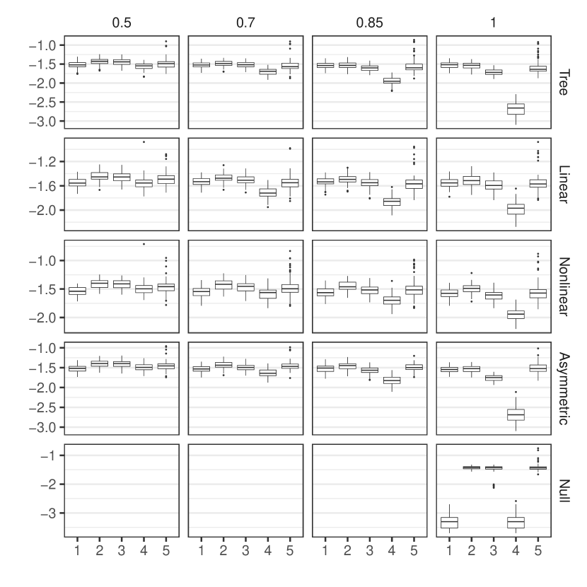
(a) $\log_{10}$ ISE${}_{\text{out}}$

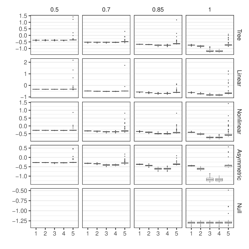
(b) $\log_{10}$MSE${}_{y\text{out}}$

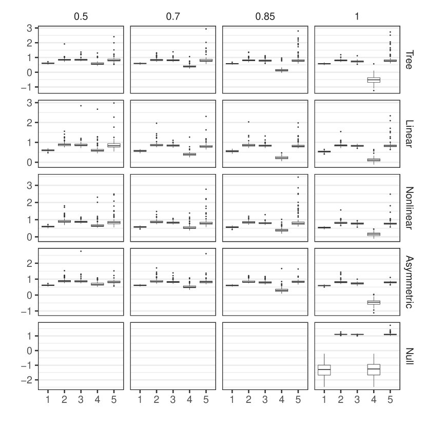
(c) $\log_{10}$ MSE_b

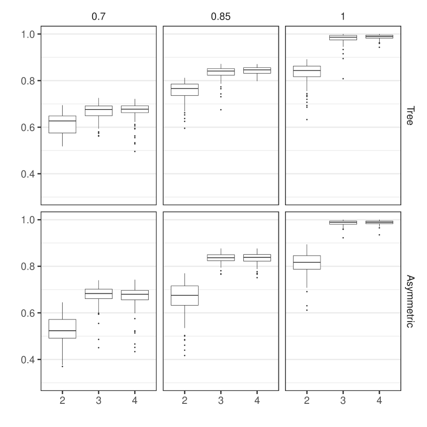
(d) Acc_g

Figure 2: Boxplots of model performance: ISE${}_{\text{out}}$, MSE${}_{y_{\text{out}}}$, and MSE_b on $\log_{10}$ scale, and Acc_g, for $N=500$, light censoring, and Weibull-I distributions. The five models are given in Table 1.

Table 2: The average running time in seconds (standard deviation in parentheses) on a data set with time-varying covariates, $N=500$, light censoring and Weibull-I distribution.

Structure	$p_{0}$	JLCT	JLCM
Tree	0.5	13.97 (0.41)	1855.64 (484.12)
	0.7	12.76 (0.36)	1777.32 (464.07)
	0.85	10.84 (0.49)	1897.43 (461.45)
	1	7.79 (0.54)	2008.06 (461.2)
Linear	0.5	23.51 (0.92)	1963.11 (437.16)
	0.7	23.27 (1.21)	1916.92 (423.97)
	0.85	21.3 (1.27)	2015.88 (366.85)
	1	20.8 (1.3)	2130.13 (519.01)
Nonlinear	0.5	13.7 (0.82)	2052.86 (342.14)
	0.7	13.6 (0.44)	2040.33 (309.27)
	0.85	12.69 (0.51)	2095.46 (368.12)
	1	11.93 (0.91)	2093.55 (393.01)
Asymmetric	0.5	13.25 (0.62)	1979.74 (198.41)
	0.7	13.37 (1.73)	1992.53 (203.28)
	0.85	13.4 (1.1)	2061.09 (204.94)
	1	8.94 (0.86)	2068.58 (165.99)
Null	1	0.61 (1.78)	1275.76 (549.94)

Null scenario

Under the null scenario where there are no latent classes, the average number of terminal nodes chosen by the four JLCT models are 1, 1.08, 1.06, 1.08, respectively, indicating that JLCT almost always makes the correct decision of not splitting. JLCT₁ and JLCT₄ have comparable performances, while JLCT₂, JLCT₃ are significantly worse, yet still comparable with JLCM, in survival prediction (ISE${}_{\text{out}}$) and survival parameter estimation (MSE_b). This is because JLCT₂, JLCT₃ and JLCM use time-invariant survival predictors ${\boldsymbol{X}^{\text{s}}}|_{\text{1st}}$, whereas JLCT₁ and JLCT₄ uses the original time-varying $\boldsymbol{X}^{\text{s}}$. This again reflects the prognostic value of time-varying covariates. By the definition of Acc_g, all JLCT models have Acc_g=1 under the null scenario, and thus we skip its discussion. As for running time, since JLCT correctly decides to not split, its running time is significantly less than when there are actual latent classes. JLCM also has reduced running time under the null scenario (roughly 35% less), but it is still much more computationally intensive than JLCT.

3.5 Additional simulation results

As mentioned in Section 2.2, we also compare performance using the default stopping criterion $\texttt{TS}_{\text{parent}}<3.84$ to two alternatives, $\texttt{TS}_{\text{parent}}<\{2.71,6.63\}$, under the above simulation setups for JLCT₄ model. Table 3 reports the average number of terminal nodes using the three stopping rules, and as can be seen, JLCT₄ splits into very similar numbers of terminal nodes regardless of the stopping criterion. As a result, the rest of the metrics are also comparable, which are given in Appendix G.

Table 3: The average number of terminal nodes (standard deviation in parentheses) using JLCT₄ in simulations based on a data set with time-varying covariates, $N=500$, light censoring and Weibull-I distribution, for three different stopping rules.

Structure	$p_{0}$	$\texttt{TS}_{\text{parent}}<2.71$	$\texttt{TS}_{\text{parent}}<3.84$	$\texttt{TS}_{\text{parent}}<6.63$
Tree	0.5	5.96 (0.2)	5.96 (0.2)	5.96 (0.2)
	0.7	5.96 (0.24)	5.96 (0.24)	5.96 (0.24)
	0.85	6 (0)	6 (0)	6 (0)
	1	4.27 (0.57)	4.15 (0.41)	4.04 (0.2)
Linear	0.5	5.94 (0.24)	5.94 (0.24)	5.93 (0.26)
	0.7	5.99 (0.1)	5.99 (0.1)	5.99 (0.1)
	0.85	5.99 (0.1)	5.99 (0.1)	5.99 (0.1)
	1	6 (0)	6 (0)	5.99 (0.1)
Nonlinear	0.5	5.76 (0.51)	5.76 (0.51)	5.77 (0.51)
	0.7	5.95 (0.22)	5.95 (0.22)	5.95 (0.22)
	0.85	5.99 (0.1)	5.99 (0.1)	5.99 (0.1)
	1	5.98 (0.28)	5.92 (0.31)	5.9 (0.36)
Asymmetric	0.5	5.86 (0.47)	5.86 (0.47)	5.84 (0.49)
	0.7	5.91 (0.29)	5.91 (0.29)	5.92 (0.27)
	0.85	5.83 (0.43)	5.84 (0.42)	5.85 (0.41)
	1	4.36 (0.63)	4.2 (0.43)	4.03 (0.17)
Null	1	1.18 (0.52)	1.08 (0.34)	1.01(0.10)

Simulations were also run based on a mix of time-invariant and time-varying covariates (results not reported). Unsurprisingly, the patterns are similar to those with all time-varying covariates.

Finally, we also examined using the median of the time-varying covariate values rather than the first encountered value when running JLCM, but the improvements in performance are negligible and the results are thus omitted.

4 Application

In this section, we illustrate the application of JLCT to a real data set, the PAQUID (Personnes Agées Quid) data set, which was also examined in [10]. The PAQUID dataset consists of 2250 records of 500 subjects from the PAQUID study [20], which collects five time-varying values, including three cognitive tests (MMSE, IST, BVRT), a physical dependency score (HIER), and a measure of depressive symptomatology (CESD), along with age at visit (age). The time-to-event is the age at dementia diagnosis or last visit, which is recorded in the tuple (agedem, dem). The PAQUID data set also collects three time-invariant covariates: education (CEP), gender (male), and age at the entry of the study (age_init). As suggested by [10], we normalize the highly asymmetric covariate MMSE and only consider its normalized version normMMSE; we also construct a new covariate $\texttt{age65}=(\texttt{age}-65)/10$. Our goal for this data set is to jointly model the trajectories of normMMSE (longitudinal outcomes) and the risk of dementia (time-to-event), using the remaining covariates.

We further compared JLCT’s performance to that of JLCM and another joint modeling baseline, the shared random effects model (SREM) [21, 22, 23, 24]. The name “shared random effects” comes from the modeling assumption that a set of random effects accounts for the association between longitudinal outcomes and time-to-event. The longitudinal outcomes are modeled by linear mixed-effects models, with random effects for each subject. These random effects affect the hazards of the event through a proportional hazard model. SREM is limited in the use of covariates in the survival model in the same way JLCM is, as it only allows time-invariant baseline covariates. [25] showed that SREM and JLCM can be viewed as special cases of a general parametric joint modeling of longitudinal and time-to-event outcomes, with the variable that ties these two parts together either being continuous (SREM) or discrete (JLCM). Thus, while SREM can represent the underlying distributions of the time-to-event and longitudinal variable, respectively, while accounting for their joint association, it does not produce the desired latent classes described in the introduction section.

4.1 Models

We consider two JLCM, one SREM, and four JLCT models.

1. (JLCM₁) We adopt the time-invariant JLCM model in [10]: The trajectories of normMMSE depend on fixed effects $\boldsymbol{X}^{\text{f}}=\{$age65, $\texttt{age65}^{2}$, CEP, male$\}$, and random effects $\boldsymbol{X}^{\text{r}}=\{$age65, $\texttt{age65}^{2}\}$. The risk of dementia depends on $\boldsymbol{X}^{\text{s}}=\{$CEP, male$\}$, with class-specific Weibull baseline hazards function. The class membership is modeled by $\boldsymbol{X}^{\text{g}}=\{$CEP, male$\}$.

2. (JLCM₂) We extend JLCM₁ to using additional covariates: the survival model uses covariates $\boldsymbol{X}^{\text{s}}=\{$CEP, male, age_init, ${\texttt{BVRT}}|_{\text{1st}}$, ${\texttt{IST}}|_{\text{1st}}$, ${\texttt{HIER}}|_{\text{1st}}$, ${\texttt{CESD}}|_{\text{1st}}$ $\}$; the class membership model uses covariates $\boldsymbol{X}^{\text{g}}=\{$CEP, male, ${\texttt{age65}}|_{\text{1st}}$, ${\texttt{BVRT}}|_{\text{1st}}$, ${\texttt{IST}}|_{\text{1st}}$, ${\texttt{HIER}}|_{\text{1st}}$, ${\texttt{CESD}}|_{\text{1st}}$ $\}$. The rest of the model remains the same as in the time-invariant JLCM₁. Note that Jointlcmm automatically uses the first encountered value ${X}|_{\text{1st}}$ of any time-varying covariate $X$.

3. (SREM) The shared random effects model (SREM). Since fitting a SREM model becomes difficult when there are multiple predictors, we consider a simple SREM model that uses the same sets of time-invariant covariates as JLCM₁: the trajectories of normMMSE depend on fixed effects $\boldsymbol{X}^{\text{f}}=\{$age65, $\texttt{age65}^{2}$, CEP, male$\}$ and the shared random effects $\boldsymbol{X}^{\text{r}}=\{$age65, $\texttt{age65}^{2}\}$. The risk of dementia depends on $\boldsymbol{X}^{\text{s}}=\{$CEP, male$\}$, as well as the shared random effects $\{$age65, $\texttt{age65}^{2}\}$. We use a Weibull baseline hazards function.

4. (JLCT₁) The first JLCT model uses the same sets of covariates as JLCM₁ and SREM.

5. (JCLT₂) The second JLCT model uses the same sets of covariates as JLCM₂. In particular, JLCT₂ also uses ${X}|_{\text{1st}}$ for any time-varying covariate $X$.

6. (JCLT₃) The third JLCT model uses the same sets of covariates as JLCM₂. However, JLCT₃ uses all values of the time-varying covariates for splitting $\boldsymbol{X}^{\text{g}}$, but it still uses ${\boldsymbol{X}^{\text{s}}}|_{\text{1st}}$ to model time-to-event outcome.

7. (JLCT₄) The last JLCT model adopts the same sets of covariates as JLCM₂, but using all values of any time-varying covariate: $\boldsymbol{X}^{\text{s}}=\{$CEP, male, age_init, BVRT, IST, HIER, CESD$\}$; and $\boldsymbol{X}^{\text{g}}=\{$CEP, male, age65, BVRT, IST, HIER, CESD$\}$. JLCT₄ is our main model with no comparable competitors.

As in the simulations, we fit the JLCM and JLCT models using the R packages lcmm and jlctree, respectively. For the two JLCM models, the number of latent classes is chosen from 2 to 6 according to the BIC selection criterion. For the four JLCT models, we set the stopping threshold to $3.84$ and prune the trees to have no more than 6 terminal nodes. For all JLCT and JLCM models, the survival models share the same slope coefficients across latent classes, a setup adopted by [10]. We fit the SREM model using the jointModel function of the JM [24] package, and then uses its associated predict.jointModel and survfitJM functions to predict longitudinal outcomes and survival curves .

4.2 Evaluation metrics

We use the root mean squared error (RMSE) to measure the accuracy of the predicted longitudinal outcomes, as was done in the simulations. However, unlike in the simulations where we know the true survival curve for each subject, in this application we only have the empirical survival curves. Thus, to evaluate the accuracy of the time-to-event predictions, we take the commonly used measure, the Brier score and its integrated version, IBS [26]. The Brier score (BS) at a fixed time $t$ is defined as

$$\text{BS}(t)=\frac{1}{N}\sum_{i=1}^{N}\Big{(}I(Y_{i}>t)-\widehat{S}(t|X_{i})\Big{)}^{2},$$

where $\widehat{S}(t|X_{i})$ is the predicted probability of survival at time $t$ conditioning on subject $i$’s predictor vector $X_{i}$, and $Y_{i}$ is the time-to-event of subject $i$. The Integrated Brier score (IBS) is therefore defined as

$$\text{IBS}=\frac{1}{\max{Y_{i}}}\int_{0}^{\max{Y_{i}}}\text{BS}(Y)dY.$$

We compute the accuracy measure on out-of-sample subjects using 10-fold cross-validation as follows. We first randomly divide the data set into 10 folds of equal size, where we take care such that observations of a single subject belong to the same fold. Next, we hold out one fold of data and run the model on the remaining nine folds. The performance of the model is then evaluated on the held out data. The procedure is repeated 10 times, where each of the 10 folds is used for out-of-sample evaluation.

4.3 Results

We report the average prediction measure and running time over the 10 folds in Table 4. When using only time-invariant covariates, JLCT₁ performs similarly to its counterpart JLCM₁ in prediction accuracy (IBS and RMSE), while SREM outperforms both JLCT₁ and JLCM₁ in survival prediction (IBS). By adding four “time-invariant” covariates (which are converted from time-varying ones) to the class membership and survival models, the performance of JLCT₂ remains similar, but the performance of JLCM₂ becomes much worse. In fact, JLCM₂’s IBS is even worse than a simple prediction of $\widehat{S}=0.5$ for every observation (which gives IBS $=0.25$), as JLCM fails to converge. When using the original time-varying covariates in the class membership, both JLCT₃ and JLCT₄ improve their time-to-event prediction accuracies and outperform all other methods by a noticeable margin on that measure. When further allowing time-varying covariates to model time-to-event outcomes, JLCT₄ gives an additional lift over JLCT₃ on time-to-event prediction. When we look at the running times, JLCT is much faster than JLCM: fitting using JLCT took no more than 2 minutes even for the most complex model (JLCT₄), while fitting using JLCM took from 40 to 60 minutes. The model fitting is performed on a desktop with 2.26GHz CPU and 32GB of memory.

The results in Table 4 demonstrate two key advantages of the tree-based approach JLCT over the parametric JLCM and SREM: JLCT is capable of providing significantly better prediction performance with the use of time-varying covariates in all of its modeling components, and it can be orders of magnitude faster to fit JLCT than to fit JLCM. Although SREM runs fast with simple models, it can be difficult to fit SREM to complex joint models, and its prediction performance from a practical point of view is therefore limited. Further, of course, it does not provide estimated latent classes at all.

Table 4: Performance of JLCM, SREM, and JLCT methods on the PAQUID data set.

	JLCM1	JLCM2	SREM	JLCT1	JLCT2	JLCT3	JLCT4
IBS	0.1731	0.4467	0.1271	0.1611	0.1690	0.1060	0.0966
RMSE	14.7588	18.3544	14.6689	14.5503	14.2912	14.5590	14.5014
Time (secs)	2448.70	4107.62	63.39	1.70	40.91	59.86	87.91

Figures 3(a)-3(d) give the four JLCT tree structures, which are fit using the entire PAQUID data set. The numbers in each box display the test statistics TS, and the proportion of observations contained in the current node. We make the following observations:

• When fitting with only time-invariant covariates CEP and male, JLCT₁ first splits into CEP$=0$ and CEP$=1$, then splits on gender within the node of $\texttt{CEP}=1$. Two of the three terminal nodes have final TS greater than the stopping criterion, 3.84, which indicates potential association between longitudinal and survival data within these two nodes. However, since CEP and male take binary values $\{0,1\}$, JLCT₁ cannot split further. Thus, it seems unlikely that using only the original time-invariant covariates provides adequate fit for these data.

• JLCT₂ uses more splitting covariates, $\boldsymbol{X}^{\text{g}}=\{$CEP, male, ${\texttt{age65}}|_{\text{1st}}$, ${\texttt{BVRT}}|_{\text{1st}}$, ${\texttt{IST}}|_{\text{1st}}$, ${\texttt{HIER}}|_{\text{1st}}$, ${\texttt{CESD}}|_{\text{1st}}$ $\}$, with some of the covariates converted from time-varying ones. JLCT₂ makes multiple splits on ${\texttt{CESD}}|_{\text{1st}}$, and then makes a final split on ${\texttt{ISE}}|_{\text{1st}}$. With additional covariates to split on, JLCT₂ ends up with five terminal nodes, each having a test statistic less than 3.84, and thus JLCT₂ has uncovered a good partitioning in the sense that the terminal nodes lack evidence of association between the longitudinal and survival outcomes. However, the prediction performance of JLCT₂ does not show improvement over JLCT₁ based on cross-validation, suggesting that the JLCT models have reached a limit with only time-invariant original and constructed covariates to use.

• Both JLCT₃ and JLCT₄ use all of the time-varying values of the $\boldsymbol{X}^{\text{g}}$ covariates in JLCT₂. The difference is that JLCT₃ only uses time-invariant values in modeling the time-to-event outcome, whereas JLCT₄ uses the time-varying counterparts. JLCT₃ first splits based on age (splitting at ages 85), and further splits based on IST for the younger group. The JLCT₄ tree splits into three nodes based only on age (splitting at ages 82 and 90), suggesting that people transition into different dementia statuses as they get older, which are reflected in both cognitive test score (normMMSE) and time until a dementia diagnosis.

• The different tree structures of JLCT₃ and JLCT₄ indicate that IST is potentially an important predictor for dementia diagnosis. Among the extended Cox PH models fit within each terminal node of JLCT₄, IST has a $p$-value of $0.02$ and $0.12$ within the groups of $\texttt{age}<82$ and $82\leq\texttt{age}<90$, respectively. In fact, it is the most statistically significant covariate among all covariates in all Cox PH models fit within each JLCT₄ terminal node, suggesting that IST is the most prognostic covariate for dementia among the younger age groups ($\texttt{age}<90$). Since JLCT₃ can only use the first encountered value of IST to model the time-to-dementia, it apparently exploits the prognostic power of IST by splitting on IST among the younger age groups. The time-to-dementia prediction accuracy of JLCT₃ is only slightly worse than that of JLCT₄, suggesting that both ways of using IST reasonably capture the relationship between IST and dementia statuses.

• All three nodes of JLCT₃ and JLCT₄ obtain a final test statistic less than 3.84, which indicates a good partitioning of the population in terms of preserving conditional independence within groups. With time-varying latent class memberships, both JLCT₃ and JLCT₄ achieve significant improvement in prediction performance of time to dementia diagnosis.

Finally, to study the effect of stopping parameter $s$ on the JLCT model, we consider two additional values: $s=2.71$ and $s=6.63$, which correspond to the 10% and 1% tails of $\chi_{1}^{2}$ distribution, respectively. Recall that the default value $s=3.84$ is the 5% tail of $\chi_{1}^{2}$ distribution. We run JLCT₄ with these three stopping values, and compare the 10-fold cross-validation results in Table 5. With a smaller $s$ value, JLCT₄ tends to split into more terminal nodes, which for this data set improves the cross-validation-estimated survival prediction performance accuracy (IBS), and slightly improves the longitudinal predictions (RMSE), although of course it is impossible to know if these small cross-validation gains correspond to real improvements in representing the underlying longitudinal and time-to-event processes.

The fitted JLCT models point out that any apparent predictive power of the cognitive assessment MMSE for time to dementia could easily be spurious, since once age is taken into account in the form of three broad age groups, any association between MMSE and agedem is gone. This suggests that the use of the MMSE test to predict time to dementia is problematic in older people. Furthermore, IST is a strong predictor for age to dementia in the two younger age groups, but not the oldest group, suggesting once again that for older people the tests have limited use for this purpose. It is known that MMSE tends to decrease with age [27], and since MMSE is widely-used, and considered a standard by which other cognitive tests are evaluated [28], our finding points to a possibly inappropriate use of this test for determining time to dementia diagnosis, which might also apply to other assessment tools as well.

Table 5: Performance of JLCT₄ on the PAQUID data set, with various values for stopping parameter $s$.

	$s=2.71$	$s=3.84$	$s=6.63$
IBS	0.0842	0.0966	0.0988
RMSE	14.4698	14.5014	14.5817
Time (secs)	87.54	87.91	51.46

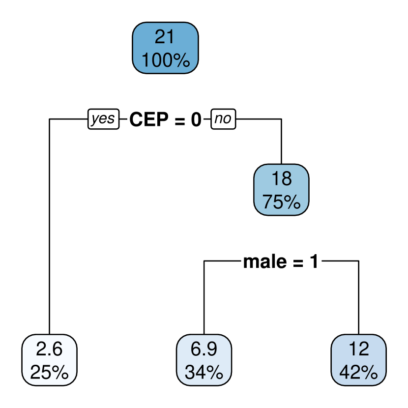
(a) JLCT₁ tree structure.

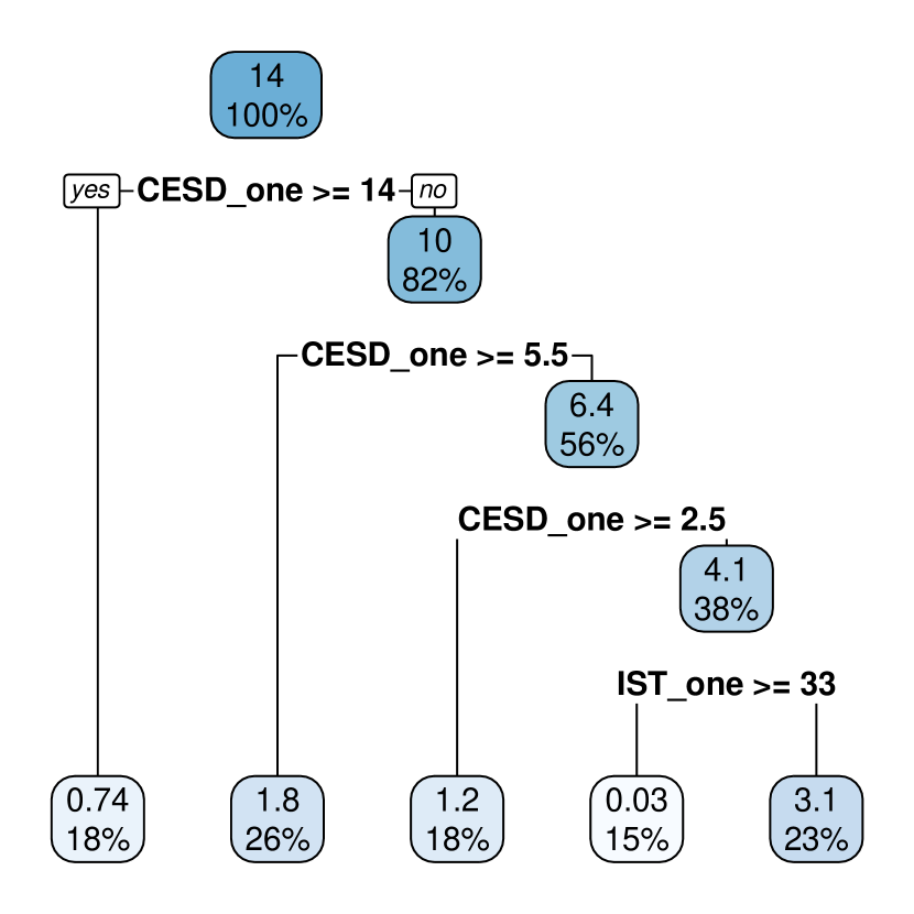
(b) JLCT₂ tree structure.

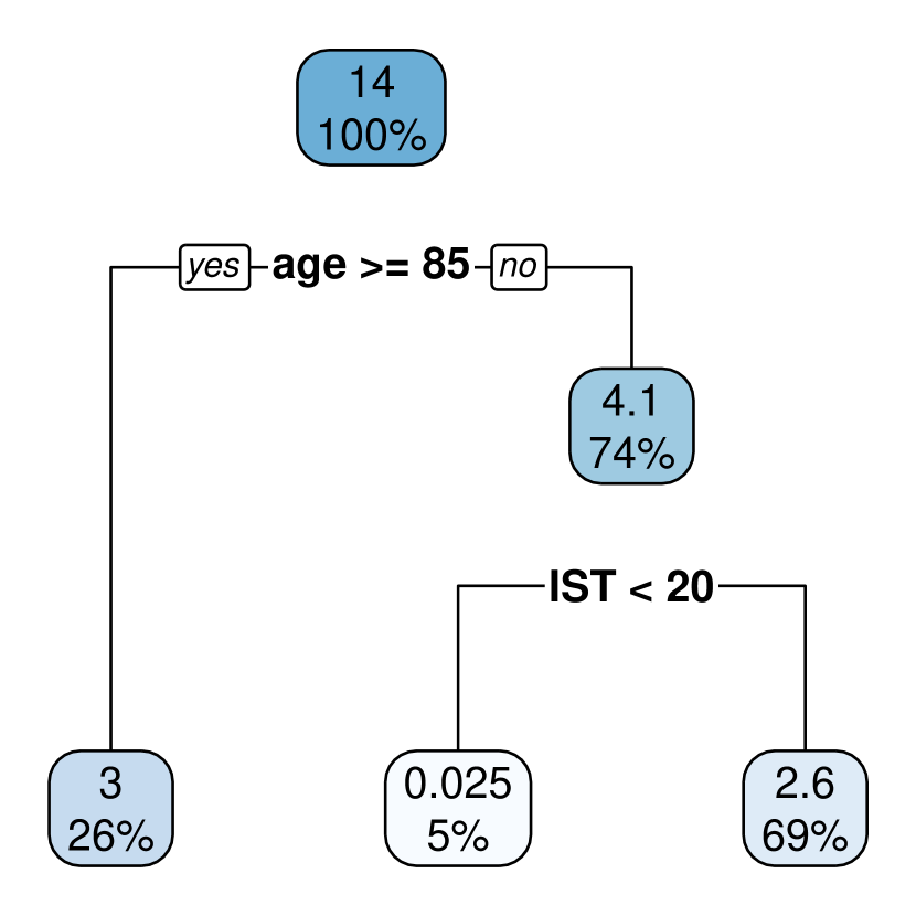
(c) JLCT₃ tree structure.

(d) JLCT₄ tree structure.

Figure 3: The tree structures returned by JLCT methods. JLCT₁: constructed with $\boldsymbol{X}^{\text{g}}=\{$CEP, male$\}$. JLCT₂: constructed with $\boldsymbol{X}^{\text{g}}=\{$CEP, male, ${\texttt{age65}}|_{\text{1st}}$, ${\texttt{BVRT}}|_{\text{1st}}$, ${\texttt{IST}}|_{\text{1st}}$, ${\texttt{HIER}}|_{\text{1st}}$, ${\texttt{CESD}}|_{\text{1st}}$ $\}$. JLCT₃ and JLCT₄: constructed with $\boldsymbol{X}^{\text{g}}=\{$CEP, male, age65, BVRT, IST, HIER, CESD $\}$.

5 Conclusion

In this paper, we have proposed a tree-based approach (JLCT) to model longitudinal outcomes and time-to-event with latent classes. Simulations and real application on the PAQUID data set show that JLCT makes full use of the time-varying information and can demonstrate significant advantages over JLCM, which can only use a subset of the available time-varying data. In addition, JLCT is orders of magnitude faster than JLCM under both scenarios.

Both JLCT and JLCM assume that the time-to-event and the longitudinal variable are independent given latent class membership. It is possible, of course, that subjects come from homogeneous latent classes within which the two variables are associated with each other. [29] proposed such a model, which generalizes JLCM by fitting a SREM for the subjects within each latent class. This adds more challenges in maximum likelihood fitting (some of which are alluded to in the paper), making this model less likely than JLCM or JLCT to scale to large data sets.

There are several interesting extensions of the JLCT method that could be explored. The PAQUID data set discussed in [10] and in Section 5 is actually one exhibiting competing risks, since there is a risk of death before dementia is exhibited, but this was ignored in the analysis. It would be of interest to generalize JLCT to account for this. Often survival values are only known to within an interval of time (interval-censoring), and JLCT could be adapted to that situation as well. In addition, the analysis here only allows for one longitudinal outcome, but sometimes several biomarkers are available for a patient, and it would be useful to generalize JLCT to allow for that. The PAQUID data is a good example of this: besides the current biomarker MMSE, both IST and BVRT are cognitive tests that can be used as biomarkers as well. One possible solution for extending JLCT to the scenario of multiple biomarkers is to perform simultaneous hypothesis tests on all biomarkers in the tree splitting procedure.

An R package, jlctree, that implements JLCT is available at CRAN. Appendix H provides code illustrating its use.

Appendix A Joint Latent Class Models (JLCM)

In this section, we give a brief introduction to JLCM, and discuss its strengths and weaknesses. More details about JLCM can be found in [30].

In JLCM, the latent class membership $g_{i}\in\{1,\dots,G\}$ for subject $i$ is determined by the set of covariates $\boldsymbol{X}^{\text{g}}_{i}$, ($\boldsymbol{X}^{\text{g}}_{it}$ must be time-invariant in JLCM, so we drop the time indicator $t$), through the following probabilistic model:

$$\pi_{ig}=\Pr(g_{i}=g|\boldsymbol{X}^{\text{g}}_{i})=\frac{\exp\{\xi_{0g}+\boldsymbol{X}^{\text{g}}_{i}\xi_{1g}\}}{\sum_{l=1}^{G}\exp\{\xi_{0l}+\boldsymbol{X}^{\text{g}}_{i}\xi_{1l}\}},$$

where $\xi_{0g},\xi_{1g}$ are class-specific intercept and slope parameters for class $g=1,\cdots,G$.

The longitudinal outcomes in JLCM are assumed to follow a slightly different linear mixed-effects model than in (2):

$$y_{it}|_{g_{i}=g}=\boldsymbol{X}^{\text{f}}_{it}\boldsymbol{\beta}_{g}+\boldsymbol{X}^{\text{r}}_{it}\boldsymbol{u}_{ig}+\varepsilon_{it},\quad\boldsymbol{u}_{ig}=\boldsymbol{u}_{i}|_{g_{i}=g}\sim\mathcal{N}(\boldsymbol{\mu}_{g},\boldsymbol{B}_{g}),\quad\varepsilon_{it}\sim\mathcal{N}(0,\sigma^{2}),$$

where $\boldsymbol{\beta}_{g}$ is the fixed effect vector for class $g$, and $\boldsymbol{u}_{ig}$ is the random effect vector for subject $i$ and class $g$. The random effect vector $\boldsymbol{u}_{ig}$ is independent across latent classes and subjects, and normally distributed with mean $\boldsymbol{\mu}_{g}$ and variance-covariance matrix $\boldsymbol{B}_{g}$. The errors $\varepsilon_{it}$ are assumed to be independent and normally distributed with mean $0$ and variance $\sigma^{2}$, and independent of all of the random effects as well. Let $f(\boldsymbol{Y}_{i}|g_{i}=g)$ denote the likelihood of longitudinal outcomes $\boldsymbol{Y}_{i}$ given that subject $i$ belongs to latent class $g$.

The time-to-event $T_{i}$ is considered to follow the proportional hazards model with time-invariant covariates $\boldsymbol{X}^{\text{s}}$:

$$h_{i}(t|g_{i}=g)=h_{0g}(t;\zeta_{g})e^{\boldsymbol{X}^{\text{s}}_{i}\eta_{g}},$$ (5)

where $\zeta_{g}$ parameterizes the class-specific baseline hazards $h_{0g}$, and $\eta_{g}$ is associated with the set of covariates $\boldsymbol{X}^{\text{s}}_{i}$ (we drop the time indicator $t$ from $\boldsymbol{X}^{\text{s}}_{it}$ since it must be time-invariant in JLCM). Let $S_{i}(t|g_{i}=g)$ denote the survival probability at time $t$ if subject $i$ belongs to latent class $g$. Note that the extended Cox model (1) of JLCT extends the proportional hazards model (5) to allow for time-varying covariates.

Let $\theta_{G}=\big{(}\xi_{0g}$, $\xi_{1g}$, $\boldsymbol{\beta}_{g}$, $\boldsymbol{u}_{ig}$, $\boldsymbol{\mu}_{g}$, $\boldsymbol{B}_{g}$, $\sigma$, $\zeta_{g}$, $\eta_{g}$: $g={1,\cdots,G}$, $i={1,\cdots,N}\big{)}$ be the entire vector of parameters of JLCM. These parameters are estimated together via maximizing the log-likelihood function

$$L(\theta_{G})=\sum_{i=1}^{N}\log\left(\sum_{g=1}^{G}\pi_{ig}f(\boldsymbol{Y}_{i}|g_{i}=g;\theta_{G})h_{i}(T_{i}|g_{i}=g;\theta_{G})^{\delta_{i}}S_{i}(T_{i}|g_{i}=g;\theta_{G})\right).$$

The log-likelihood function above uses the assumption that conditioning on the latent class membership ($g_{i}$), longitudinal outcomes ($\boldsymbol{Y}_{i}$) and time-to-event ($T_{i},\delta_{i}$) are independent.

As mentioned in the introduction, the concept of latent class membership is of particular interest in clinical studies. JLCM is designed to give parametric descriptions of subjects’ tendency of belonging to each latent class, and therefore JLCM is a suitable model when the true latent class is indeed a random outcome with unknown probabilities for each class. The multinomial logistic regression that JLCM uses is a flexible tool to model these unknown probabilities.

Despite the usefulness of latent classes, JLCM has several weaknesses. First of all, the running time of JLCM does not scale well due to its complicated likelihood function. Simulation results show that the running time of JLCM increases exponentially fast as a function of the number of observations, the number of covariates, and the number of assumed latent classes [11]. Secondly, the modeling of time-to-event in JLCM is restricted to the use of time-invariant covariates. However, time-varying covariates are helpful in modeling the time-to-event, especially when treatment or important covariates change during the study, for instance the patient receives a heart transplant [31], or the longitudinal CD4 counts change during the study of AIDS [32]. Research shows that using time-varying covariates can uncover short-term associations between time-to-event and covariates [33, 34], and ignoring the time-varying nature of the covariates will lead to time-dependent bias [35, 36]. The other restriction of JLCM is that the latent class membership model only uses time-invariant covariates, which implies that the latent class membership of a subject is assumed to be fixed throughout the time of study. However, the stage of a disease of a patient is very likely to change during the course of clinical study, for instance the disease would move from its early stages to its peak, and then move to its resolution. When the goal of joint modeling is to uncover meaningful clustering of the population that leads to definitions of disease stages, it is important to allow time-varying covariates in the latent class membership model, so that the model reflects this real world situation.

Although JLCM does not allow time-varying covariates in fitting time-to-event outcomes and latent class memberships, its implementation in the R package lcmm can take in time-varying covariates. In that case, lcmm will automatically take the first encountered values of those covariates of each subject and use them as if these covariates are time-invariant.

Appendix B Convert data into the left-truncated right-censored (LTRC) format

Here we describe how to convert the original survival data with time-varying covariates into the left-truncated right-censored (LTRC) format.

For each subject $i$ and measurement time $t$, there is a “pseudo-observation” with $y_{it},\boldsymbol{X}_{it}$, and a time-to-event triplet $(L_{it},R_{it},\delta_{it})$, where $L_{it}$ is the left-truncated time, $R_{it}$ is the right-censored time, and $\delta_{it}$ is the censor indicator. Table 6 illustrates how to convert the time-to-event data (Time, Death) with a time-varying covariate (CD4) into the LTRC format. The left chart shows that the subject with $\text{ID}=1$ is observed at times 0, 10, and 20, respectively, with Age and CD4 recorded, and the death occurred at time 27. The right chart shows the corresponding LTRC format, where each pseudo-observation is left-truncated (at time $L$) and right-censored (at time $R$), with the corresponding covariates (Age, CD4) and censor indicator $\delta$.

Table 6: Converting the original data (left chart) into the left-truncated right-censored (LTRC) format (right chart).

ID	Age	CD4	Time	Death($\delta$)
1	45	27	0	0
1	45	31	10	0
1	45	25	20	0
1	-	-	27	1

$\Rightarrow$ ID Age CD4 $L$ $R$ Death($\delta$) 1 45 27 0 10 0 1 45 31 10 20 0 1 45 25 20 27 1

Appendix C Simulation setup: time-invariant covariates

In this section we give details of the data generating scheme in the simulation study of time-invariant covariates only.

C.1 Data

At each simulation run, for each subject $i$ we randomly generate five independent, time-invariant covariates $X_{i1},\dots,X_{i5}$. We assume there are four latent classes $g=1,\dots,4$, which are determined by covariates $X_{1},X_{2}$. Once the latent classes are determined for each subject $i$, the time-to-event and the longitudinal outcomes are conditionally independent given the latent classes, and therefore generated separately. In particular, the survival outcomes (time-to-event) depend on $X_{3},X_{4},X_{5}$, and the longitudinal outcomes depend on the latent classes. We give more details below.

Covariates

At each simulation run, for each subject $i$ we draw $X_{i1}$, $X_{i2}$, $X_{i3}$, $X_{i4}$, $X_{i5}$ uniformly from $[0,1]$, $[0,1]$, $\{0,1\}$, $[0,1]$, and $\{1,2,3,4,5\}$ respectively.

Latent classes

We determine class membership based on a multinomial logistic model of $X_{1},X_{2}$, with increasing level of concentration on one class. Our latent class membership generation model matches the setup of JLCM, and it approaches the setup of JLCT as the concentration level approaches $1$.

For subject $i$, we compute the value of a “score” function $f(w_{g},X_{i1},X_{i2})$, where $w_{g}$ denotes the parameters associated with latent class $g$, and $X_{i1},X_{i2}$ denote the first two covariates of subject $i$. The latent class membership for subject $i$, $g_{i}$, is generated according to two key values: the “majority” class $g_{i}^{0}$, and the “concentration” level $p_{0}$. We define the “majority” class as the latent class with largest score for sample $i$,

$$g_{i}^{0}=\operatorname*{arg\,max}_{g\in\{1,2,3,4\}}f(w_{g},X_{i1},X_{i2}).$$

We consider four types of score functions $f$, which correspond to four underlying structures of latent classes: tree partition, linear separation, non-linear separation, and asymmetric tree partition. The structure is reflected by the dependency of $g_{i}^{0}$ on $X_{1},X_{2}$, which is shown in Figure 1.

The latent class membership of subject $i$ is drawn according to the probabilities

$$\Pr(g_{i}=g\mid X_{i},C)=\frac{\exp\big{\{}Cf(w_{g},X_{i1},X_{i2})\big{\}}}{\sum_{l=1}^{4}\exp\big{\{}Cf(w_{l},X_{i1},X_{i2})\big{\}}},$$

where the parameter $C$ is chosen such that the probability of “major” class is approximately equal to a pre-specified concentration level $p_{0}\in\{0.25,0.5,0.7,0.85,1\}$. That is $\Pr(g_{i}=g_{i}^{0}\mid X_{i},C)\approx p_{0}$. In particular, when $C=0$, $\Pr(g_{i}=g_{i}^{0})=0.25$, and therefore the latent class membership is randomly determined and independent of $X_{1},X_{2}$. On the other hand, when $C=\infty$, $\Pr(g_{i}=g_{i}^{0})=1$, and therefore the latent class membership corresponds to a deterministic partitioning based on $X_{1},X_{2}$, which is consistent with the assumptions underlying a tree partitioning. The choices of parameters $w_{g}$ for each latent class structure are given below.

• Tree. Consider the following coefficients $(w_{g1},w_{g2})$:

  $$w_{11}=-1,\ w_{12}=-1$$

  $$w_{21}=-1,\ w_{22}=1,$$

  $$w_{31}=1,\ w_{32}=-1,$$

  $$w_{41}=1,\ w_{42}=1.$$

  Define the score function

  $$f_{\text{tree}}(w_{g},X_{i1},X_{i2})=w_{g1}(2X_{i1}-1)+w_{g2}(2X_{i2}-1),$$

  and let $g_{i}^{0}=\operatorname*{arg\,max}_{g}f_{\text{tree}}(w_{g},X_{i1},X_{i2})$ denote the latent class with largest score for sample $i$. See Figure 1(a) for the dependency of $g_{i}^{0}$ on $X_{1},X_{2}$. The latent classes are drawn according to the probabilities

  $$\Pr(g_{i}=g\mid X_{i},C)=\frac{\exp\big{\{}Cf_{\text{tree}}(w_{g},X_{i1},X_{i2})\big{\}}}{\sum_{l=1}^{4}\exp\big{\{}Cf_{\text{tree}}(w_{l},X_{i1},X_{i2})\big{\}}},$$

  where the parameter $C$ is chosen such that $\Pr(g_{i}=g_{i}^{0}\mid X_{i},C)\approx p_{0}$, and $p_{0}$ is some pre-specified level $p_{0}\in\{0.25,0.5,0.7,0.85,1\}$. In particular, when $C=0$, $\Pr(g_{i}=g_{i}^{0})=0.25$; when $C=\infty$, $\Pr(g_{i}=g_{i}^{0})=1$.

• Linear. Consider the following coefficients $(w_{g1},w_{g2})$ drawn randomly from the unit sphere,

  $$w_{11}=0.8,\ w_{12}=-0.6$$

  $$w_{21}=0.9,\ w_{22}=0.5,$$

  $$w_{31}=-0.8,\ w_{32}=0.6,$$

  $$w_{41}=0.5,\ w_{42}=0.9.$$

  Define the score function

  $$f_{\text{linear}}(w_{g},X_{i1},X_{i2})=w_{g1}(2X_{i1}-1)+w_{g2}(2X_{i2}-1),$$

  and let $g_{i}^{0}=\operatorname*{arg\,max}_{g}f_{\text{linear}}(w_{g},X_{i1},X_{i2})$. See Figure 1(b) for the dependency of $g_{i}^{0}$ on $X_{1},X_{2}$. The latent classes are drawn according to the following probabilities

  $$\Pr(g_{i}=g\mid X_{i},C)=\frac{\exp\big{\{}Cf_{\text{linear}}(w_{g},X_{i1},X_{i2})\big{\}}}{\sum_{l=1}^{4}\exp\big{\{}Cf_{\text{linear}}(w_{l},X_{i1},X_{i2})\big{\}}},$$

  with $C$ again chosen to control the value of $\Pr(g_{i}=g_{i}^{0}\mid X_{i},C)\approx p_{0}\in\{0.25,0.5,0.7,0.85,1\}$.

• Nonlinear. We can skip the step of defining the score function $f$ and the $C$ value, but directly work with $g_{0}$ and $p_{0}$. For each observation, its “most likely” latent class $g^{0}_{i}$ is determined by whether $(X_{i1},X_{i2})$ belongs to the circles centered at $(0,0)$ and $(0,1)$ with radius $0.75$ :

  $$g_{i}^{0}=\begin{cases}1,\ \left\{X_{i1}^{2}+X_{i2}^{2}\leq 0.75^{2}\right\}\,\&\,\left\{X_{i1}^{2}+(1-X_{i2})^{2}>0.75^{2}\right\}\\ 2,\ \left\{X_{i1}^{2}+(1-X_{i2})^{2}\leq 0.75^{2}\right\}\,\&\,\left\{X_{i1}^{2}+X_{i2}^{2}>0.75^{2}\right\}\\ 3,\ \left\{X_{i1}^{2}+X_{i2}^{2}>0.75^{2}\right\}\,\&\,\left\{X_{i1}^{2}+(1-X_{i2})^{2}>0.75^{2}\right\}\\ 4,\ \left\{X_{i1}^{2}+X_{i2}^{2}\leq 0.75^{2}\right\}\,\&\,\left\{X_{i1}^{2}+(1-X_{i2})^{2}\leq 0.75^{2}\right\}\\ \end{cases}$$

  See Figure 1(c) for visualization of $g_{i}^{0}$. The latent classes are drawn according to the following probabilities:

  $$\Pr(g_{i}=g\mid X_{i})=p_{0}\{g=g^{0}_{i}\}+\frac{1-p_{0}}{3}\{g\neq g^{0}_{i}\},$$

  where $p_{0}\in\{0.25,0.5,0.7,0.85,1\}$.

• Asymmetric. We can skip the step of defining the score function $f$ and the $C$ value, but directly work with $g_{0}$ and $p_{0}$. For each observation, its “most likely” latent class $g_{i}^{0}$ is determined by the following asymmetric tree:

  $$g_{i}^{0}=\begin{cases}1,\ \{X_{i1}>0.75\},\\ 2,\ \{X_{i1}\leq 0.75\}\,\&\,\{X_{i2}\leq 0.33\},\\ 3,\ \{X_{i1}\leq 0.75\}\,\&\,\{0.33<X_{i2}\leq 0.67\},\\ 4,\ \{X_{i1}\leq 0.75\}\,\&\,\{X_{i2}>0.67\}.\end{cases}$$

  See Figure 1(d). The latent classes are drawn according to the following probabilities:

  $$\Pr(g_{i}=g\mid X_{i})=p_{0}\{g=g^{0}_{i}\}+\frac{1-p_{0}}{3}\{g\neq g^{0}_{i}\},$$

  where $p_{0}\in\{0.25,0.5,0.7,0.85,1\}$.

Time-to-event

The survival time (time-to-event) $T_{i}$ of subject $i$ follows the proportional hazards model

$$h(t,\boldsymbol{X}_{i})=h_{0}(t)e^{b_{g_{i}3}X_{i3}+b_{g_{i}4}X_{i4}+b_{g_{i}5}X_{i5}},$$

where the slope coefficients $b_{g_{i}3},b_{g_{i}4},b_{g_{i}5}$ depend on latent class $g_{i}\in\{1,2,3,4\}$ for subject $i$.

We use three different distributions for baseline hazards $h_{0}(t)$: exponential, Weibull with decreasing hazards with time (Weibull-D), and Weibull with increasing hazards with time (Weibull-I). We select parameters and slopes such that the mean values of survival time $T$ across latent classes remain similar across different distributions. The distributions and corresponding parameters for generating time-to-event data are listed below.

• Exponential with $\lambda=0.1$, and slopes are

  $$b_{13} =0,\ b_{14}=0,\ b_{15}=0$$

  $$b_{23} =0.56,\ b_{24}=0.56,\ b_{25}=0.09,$$

  $$b_{33} =0.92,\ b_{34}=0.92,\ b_{35}=0.15,$$

  $$b_{43} =1.46,\ b_{44}=1.46,\ b_{45}=0.24.$$

• Weibull distribution with shape parameter $\alpha=0.9$, which corresponds to decreasing hazards with time (Weibull-D). The scale parameter is $\beta=1$, and slopes are

  $$b_{13} =-1.17,\ b_{14}=-1.17,\ b_{15}=-0.19$$

  $$b_{23} =-0.66,\ b_{24}=-0.66,\ b_{25}=-0.11,$$

  $$b_{33} =-0.55,\ b_{34}=-0.55,\ b_{35}=-0.09,$$

  $$b_{43} =0,\ b_{44}=0,\ b_{45}=0.$$

• Weibull distribution with shape parameter $\alpha=3$, which corresponds to increasing hazards with time (Weibull-I). The scale parameter is $\beta=2$, and slopes are

  $$b_{13} =-3.22,\ b_{14}=-3.22,\ b_{15}=-0.54$$

  $$b_{23} =-2.26,\ b_{24}=-2.26,\ b_{25}=-0.38,$$

  $$b_{33} =-1.53,\ b_{34}=-1.53,\ b_{35}=-0.26,$$

  $$b_{43} =0,\ b_{44}=0,\ b_{45}=0.$$

Left truncation times are generated independently from uniform $U[0,1]$. Right censoring times are generated independently from an exponential distribution, with parameters chosen to reflect light censoring (approximately 20% observations are censored), and heavy censoring (approximately 50% observations are censored).

Longitudinal outcomes

The longitudinal outcome $y$ comes from the following linear mixed-effects model: for subject $i$ at time $t$, let $g_{i}$ denote the latent class membership, and

$$y_{it} =u_{g_{i}}+v_{i}+\varepsilon_{it},\quad v_{i}\sim\mathcal{N}(0,\sigma_{v}^{2}),\quad\varepsilon_{it}\sim\mathcal{N}(0,\sigma_{e}^{2}),$$

where $\sigma_{v}=0.2,\sigma_{e}=0.1$, and $u_{1}=0,\ u_{2}=1,\ u_{3}=1,\ u_{4}=2$ are class-specific random intercepts. We assume each subject $i$ is measured at its entry (left truncation) time, together with multiple intermediate measurement times $t_{i1},t_{i2}$, etc. The number of intermediate measurements for subject $i$ is generated independently from $1+\text{Poisson}(1)$, thus each subject has at least 2 measurements, and has 3 measurements on average. The intermediate measurement time $t_{ij}$ is then sampled independently and uniformly between subject $i$’s left-truncated and right-censored time, $t_{ij}\sim U[L_{i},T_{i}]$. Finally, the data are converted to the LTRC format according to Appendix B.

Observe that covariates $X_{1}$ and $X_{2}$ determine the latent classes, and thus affect the time-to-event and longitudinal outcomes $y$. Therefore, time-to-event is correlated with $y$ if $X_{1}$ and $X_{2}$ are unknown. On the other hand, conditioning on one of the four latent classes $g=1,2,3,4$, time-to-event and longitudinal outcomes are independent: the former follows a class-specific proportional hazards model and only depends on $X_{3},X_{4},X_{5}$, while the latter is a constant plus random noise. Therefore, the simulated data satisfy the conditional independence assumption made by both JLCM and JLCT.

C.2 Methods

JLCT and JLCM use the same subsets of covariates as in the time-varying case: $\boldsymbol{X}^{\text{s}}=\{X_{3},X_{4},X_{5}\}$, $\boldsymbol{X}^{\text{f}}=\boldsymbol{X}^{\text{r}}=\{X_{1},\dots,X_{5}\}$, ${\boldsymbol{X}^{\text{g}}}^{(\text{JLCT})}=\{X_{1},\dots,X_{5}\}$, and ${\boldsymbol{X}^{\text{g}}}^{(\text{JLCM})}=\{X_{1},\dots,X_{5},X_{1}X_{2}\}$.

We compare four methods on the simulated data set.

1. A baseline JLCT with no splitting.

2. A full JLCT model with default splitting and stopping criterion. In the second step, we fit a Cox proportional hazards (PH) model with the same baseline hazard function but different slopes across terminal nodes.

3. A full JLCT model with default splitting and stopping criterion. In the second step, we fit a Cox PH model where both baseline hazard functions and Cox PH slopes differ across terminal nodes.

4. A JLCM model. Since all the simulated covariates are time-invariant, we can fit JLCM using the original data.

C.3 Predictions

JLCT prediction

The prediction procedure for JLCT is as follows. Once JLCT returns a tree, each subject $i$ is assigned to a tree leaf node $d_{i}$. We fit the proportional hazards model (1) to the time-to-event data $(T_{i},\delta_{i})$, with time-invariant covariates $\boldsymbol{X}^{\text{s}}_{i}=\{X_{i3},X_{i4},X_{i5}\}$ and slopes $\eta_{d_{i}}=(b_{d_{i}3},b_{d_{i}4},b_{d_{i}5})$ for $d_{i}\in\{1,2,3,4,5,6\}$ (since there are no more than six terminal nodes). Method 2 assumes a shared baseline hazard function $h_{0}(t)$, meanwhile Method 3 assumes class-specific baseline hazard functions $h_{d_{i}0}(t)$. We use the R function coxph from the survival package [37, 38] to get fitted slopes $\hat{b}_{d3},\hat{b}_{d4},\hat{b}_{d5}$ for all $d\in\{1,2,3,4,5,6\}$. Given the fitted model, we compute the predicted survival probability for subject $i$ at time $t$, denoted $\hat{S}_{i}(t)$, using the R function survfit.coxph. For longitudinal outcomes, we fit the linear mixed-effects model (2) using the R function lmer from the lme4 package [39], and compute the predicted longitudinal outcomes $\hat{y}_{it}$. For any out-of-sample subject $k$, we first determine its leaf node assignment $d_{k}$ according to its covariates $\boldsymbol{X}^{\text{g}}_{k}$ and the constructed tree of JLCT. Then we proceed to compute predictions $\hat{S}_{k}(t)$ and $\hat{y}_{kt}$ as we did for the in-sample subjects.

JLCM prediction

The prediction procedure for JLCM is very similar to that of JLCT. Let $D^{*}$ be the BIC optimal number of latent classes. For each latent class $d\in\{1,\dots,D^{*}\}$, JLCM returns estimated Cox PH coefficients $\hat{b}_{d3},\hat{b}_{d4},\hat{b}_{d5}$ as well as the baseline survival curves $\hat{S}_{d0}(t)$. In addition, JLCM returns a fitted linear mixed-effects model for longitudinal outcomes. For in-sample subjects, JLCM also returns a predicted latent class membership $d_{i}$ for each subject $i$, conditioning on all available information: covariates $\boldsymbol{X}_{i}$, time-to-event $(T_{i},\delta_{i})$, and longitudinal outcomes $\boldsymbol{Y}_{i}$. We can therefore use the estimated parameters for class $d_{i}$ to compute $\hat{S}_{i}(t)|_{d_{i}}$ and $\hat{y}_{it}|_{d_{i}}$. Note that JLCM uses much more information than JLCT at the prediction time to determine the latent class memberships for in-sample subjects, and thus JLCM is expected to perform better than JLCT on in-sample data. For any new subject $k$, however, time-to-event and longitudinal outcomes are no longer available at prediction time. Instead, we use JLCM’s fitted multinomial logistic model to get $\pi_{k}=(p_{k1},\dots,p_{kD^{*}})$, a vector of predicted probabilities of subject $k$ belonging to each latent class. Finally we take weighted averages over all classes as final predictions:

$$\hat{S}_{k}(t) =\sum_{d=1}^{D^{*}}p_{kd}\ \hat{S}_{k}(t)|_{d},\quad\hat{y}_{k}(t)=\sum_{d=1}^{D^{*}}p_{kd}\ \hat{y}_{kt}|_{d}.$$

Appendix D Simulation setup: time-varying covariates

In this section we give details of the data generating scheme in the simulation study of time-varying covariates.

Covariates

At each simulation run, for each subject $i$ we randomly generate five independent, time-varying covariates $X_{it1},\dots,X_{it5}$, which are piecewise constant, and change values at time $t_{i}$. To be more concrete, for each subject $i$, we first randomly generate a time point $t_{i}\sim U[1,3]$. Next, draw $X_{i1}^{\prime}$, $X_{i2}^{\prime}$, $X_{i3}^{\prime}$, $X_{i4}^{\prime}$, $X_{i5}^{\prime}$ uniformly from $[0,1]$, $[0,1]$, $\{0,1\}$, $[0,1]$, and $\{1,2,3,4,5\}$ respectively. Generate $X_{i1}^{\prime\prime}$, $X_{i2}^{\prime\prime}$, $X_{i3}^{\prime\prime}$, $X_{i4}^{\prime\prime}$, $X_{i5}^{\prime\prime}$ by

$$X_{i1}^{\prime\prime} =\text{Proj}_{[0,1]}\Big{(}X_{i1}^{\prime}+U[-0.3,0.3]\Big{)},$$

$$X_{i2}^{\prime\prime} =\text{Proj}_{[0,1]}\Big{(}X_{i2}^{\prime}+U[-0.3,0.3]\Big{)},$$

$$X_{i3}^{\prime\prime} =U\{0,1\},$$

$$X_{i4}^{\prime\prime} =\text{Proj}_{[0,1]}\Big{(}X_{i4}^{\prime}+U[-0.3,0.3]\Big{)},$$

$$X_{i5}^{\prime\prime} =\text{Proj}_{[1,5]}\Big{(}X_{i5}^{\prime}+U\{-1,0,1\}\Big{)},$$

where the projection operator Proj${}_{[a,b]}(x)$ projects any real value $x$ onto the interval $[a,b]$. For example, Proj${}_{[0,1]}(1.3)=1$. For $k\in\{1,2,3,4,5\}$, the time-varying covariate $X_{k}$ of object $i$ at time $t$ is defined as

$$X_{itk} =1\{t\leq t_{i}\}X_{ik}^{\prime}+1\{t>t_{i}\}X_{ik}^{\prime\prime}.$$

Therefore, for each subject $i$, the five time-varying covariates $X_{1},\cdots,X_{5}$ are piecewise constant, and change values at time point $t_{i}$.

Latent classes

We use the same procedure as is described in Appendix C to generate latent classes, the only difference being that the covariates $X_{1},X_{2}$ become time-varying, as does the latent class membership. We denote by $g_{it}$ the latent class membership of subject $i$ at time $t$.

Time-to-event

The time-to-event data follow the same hazard models as in Appendix C, except that the covariates and slope coefficients are time-varying. The hazard of subject $i$ at time $t$ becomes

$$h(t,\boldsymbol{X}_{i})=h_{0}(t)e^{b_{g_{it}3}X_{it3}+b_{g_{it}4}X_{it4}+b_{g_{it}5}X_{it5}},$$

where the slope coefficients $b_{g_{it}3},b_{g_{it}4},b_{g_{it}5}$ depend on latent class membership $g_{it}\in\{1,2,3,4\}$ at time $t$.

Longitudinal outcomes

The longitudinal outcome $y$ follows the same linear mixed-effects model as in Appendix C, the only difference being now the fixed effect $u_{g_{it}}$, which depends on the latent class membership $g_{it}$, becomes time-varying as well.

Appendix E Simulation results: time-invariant covariates

In this section, we present the complete simulation results: for three time-to-event distributions (Weibull-I, Weibull-D, and Exponential), and light censoring. The results of other censoring levels (no censoring, heavy censoring) are very similar to those of light centering, and are omitted. We report results for the four methods discussed in Appendix C.2:

1. JLCT with no split,

2. JLCT with same baseline hazard function but different Cox PH slopes across terminal nodes,

3. JLCT with different baseline hazard function and different Cox PH slopes across terminal nodes,

4. JLCM with different baseline hazard function and different Cox PH slopes across terminal nodes,

We use the performance measures described in Section 3.3: ISE${}_{\text{in}}$, ISE${}_{\text{out}}$, MSE${}_{y\text{in}}$, MSE${}_{y\text{out}}$, and MSE_b. The results are given below.

Table 7: The average running time in seconds (standard deviation in parentheses) on a data set with time-invariant covariates, $N=500$, light censoring, and Weibull-I distribution.

Structure	$p_{0}$	JLCT	JLCM
Tree	0.5	14.79 (0.41)	1759.23 (354.93)
	0.7	14.12 (0.27)	2146.55 (423.37)
	0.85	13.91 (0.55)	1783.7 (432.72)
	1	9.25 (0.5)	1580.72 (333.41)
Linear	0.5	23.34 (0.59)	1609.96 (297.82)
	0.7	22.36 (0.75)	2045.23 (402.44)
	0.85	21.51 (0.99)	1752.89 (476.53)
	1	20.91 (1.41)	1694.08 (389.78)
Nonlinear	0.5	14.74 (0.71)	1489.01 (323.39)
	0.7	14.18 (0.34)	1522.28 (293.78)
	0.85	13.74 (0.39)	1597.38 (285.09)
	1	12.52 (0.87)	2985.69 (572.36)
Asymmetric	0.5	15.07 (3.44)	1494.52 (384.03)
	0.7	13.96 (0.39)	1550.19 (421.94)
	0.85	13.35 (0.72)	1719.99 (418.76)
	1	9.98 (0.59)	2559.32 (696.39)

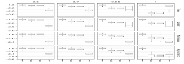
(a) Weibull-I, ISE${}_{\text{in}}$

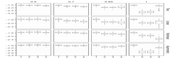
(b) Weibull-I, ISE${}_{\text{out}}$

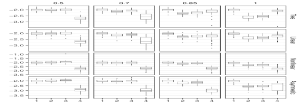
(c) Weibull-D, ISE${}_{\text{in}}$

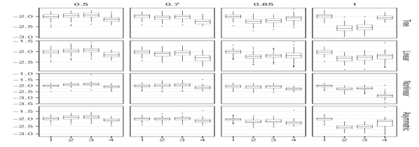
(d) Weibull-D, ISE${}_{\text{out}}$

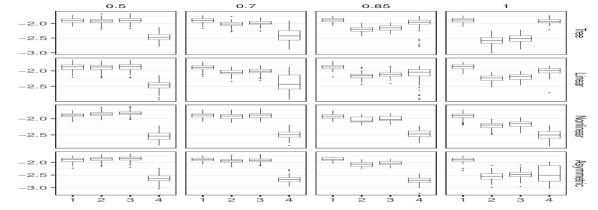
(e) Exponential, ISE${}_{\text{in}}$

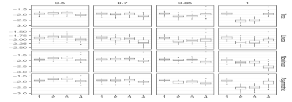
(f) Exponential, ISE${}_{\text{out}}$

Figure 4: Boxplots of integrated squared error (ISE, both in-sample and out-of-sample) on $\log_{10}$ scale, time-invariant covariates, N=500, light censoring, Weibull-I, Weibull-D, and Exponential distribution.

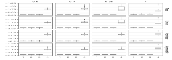
(a) Weibull-I, MSE${}_{y\text{in}}$

(b) Weibull-I, MSE${}_{y\text{out}}$

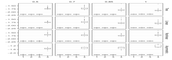
(c) Weibull-D, MSE${}_{y\text{in}}$

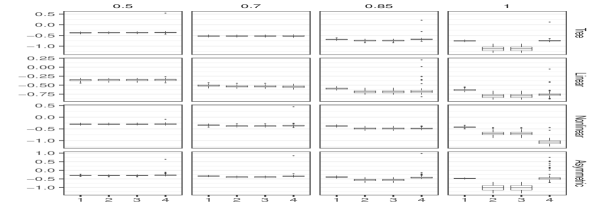
(d) Weibull-D, MSE${}_{y\text{out}}$

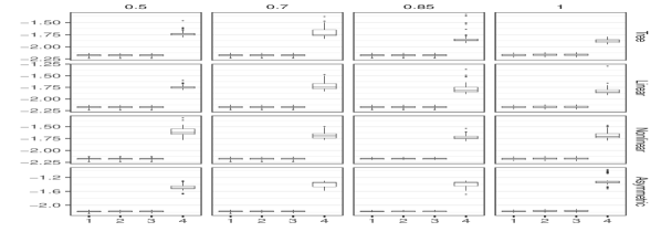
(e) Exponential, MSE${}_{y\text{in}}$

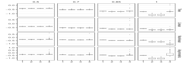
(f) Exponential, MSE${}_{y\text{out}}$

Figure 5: Boxplots of mean squared error (MSE_y, both in-sample and out-of-sample) on $\log_{10}$ scale, time-invariant covariates, N=500, light censoring, Weibull-I, Weibull-D, and Exponential distribution.

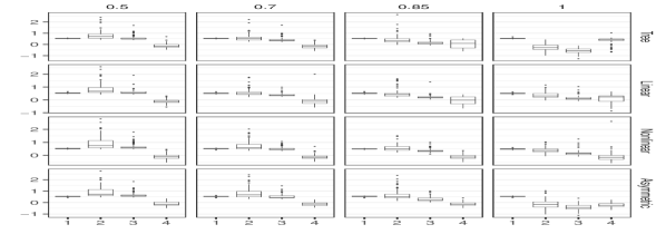
(a) Weibull-I, MSE_b

(b) Weibull-D, MSE_b

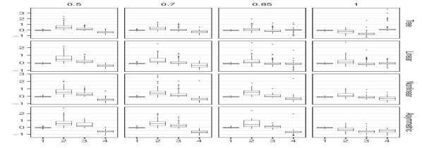
(c) Exponential, MSE_b

Figure 6: Boxplots of mean squared error (MSE_b) of estimated Cox PH slopes on $\log_{10}$ scale, time-invariant covariates, N=500, light censoring, Weibull-I, Weibull-D, and Exponential distribution.

Boxplots for ISE${}_{\text{out}}$ show that the accuracies of survival predictions of JLCT (Methods 2 & 3) and JLCM (Method 4) are comparable, with JLCT being slightly worse, under the settings where latent classes are generated from probabilistic models ($p_{0}<1$). In particular, when the latent class structure comes from a linear separation (Linear) and therefore the simulated data matches exactly the model of JLCM, JLCT still performs comparably to JLCM (e.g. $p_{0}=0.85$, “Linear”). The gap between JLCT and JLCM decreases as the concentration level increases from $p_{0}=0.5$ to $1$. In the case where $p_{0}=1$ and thus latent classes are generated by a deterministic partitioning, JLCT is more effective than JLCM in all settings except nonlinear partitioning. In particular, when the latent class model follows the deterministic partitioning by a tree ($p_{0}=1$,“Tree”) and thus matches the model of JLCT, JLCT outperforms JLCM by a significant margin. Furthermore, JLCM tends to have higher variance in ISE values, due to occasionally unconverged JLCM runs. A similar pattern appears for MSE${}_{y\text{out}}$, with JLCT and JLCM comparable for most settings, and JLCT significantly outperforming JLCM when the simulated data come from the underlying model of JLCT. Regarding estimation accuracy of Cox PH slopes (MSE_b) the same pattern shows up here as well, although there exist more outliers in all methods.

Table 7 shows the average running time of JLCT and JLCM (over 100 runs) under the same settings as the plots. The running time of JLCT includes constructing the tree, fitting the two survival models of Methods 2 and 3, and fitting the linear mixed model. The running time of JLCM includes fitting with all numbers of latent classes $g\in\{2,3,4,5,6\}$. Clearly, JLCT is orders of magnitude faster than JLCM across all settings: JLCT completes one run within a minute, while JLCM typically takes 25 to 45 minutes. The running time for other censoring levels and baseline hazard distributions are similar.

Finally, note that Methods 2 and 3 give very similar results, as they only differ in the survival models that are fitted after tree construction. Method 2 assumes a single baseline hazard function shared across terminal nodes, which agrees with the true data generating scheme. Nevertheless, Methods 2 and 3 have almost identical out-of-sample performances, which suggests that introducing additional parameters for node-specific baseline hazard functions does not hurt the prediction performance for the simulated data. In practice, it is often unclear whether the latent classes share a single baseline hazard function. Our results suggest that in such a case, we can assume a separate baseline hazard function for each terminal node, without worrying about over-fitting the data. Thus, in the time-varying simulations, we only consider the Cox PH model with separate baseline hazard functions across terminal nodes.

Appendix F Additional simulation results: time-varying covariates

In this section, we present the complete simulation results for time-varying covariates: for three time-to-event distributions (Weibull-I, Weibull-D, and Exponential), and light censoring. No censoring and heavy censoring are omitted because of their similar performances to light censoring. We report results for the five methods discussed in Table 1:

1. JLCT with no split, and using time-varying survival covariates,

2. JLCT with “time-invariant” latent class and survival covariates,

3. JLCT with “time-invariant” latent class covariates and time-varying survival covariates,

4. JLCT with time-varying latent class and survival covariates,

5. JLCM with “time-invariant” latent class and survival covariates.

We use the performance measures described in Section 3.3: ISE${}_{\text{in}}$, ISE${}_{\text{out}}$, MSE${}_{y\text{in}}$, MSE${}_{y\text{out}}$, and MSE_b.

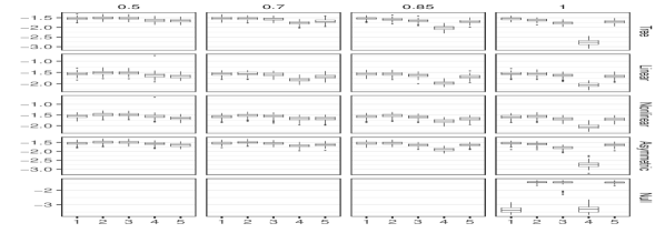
(a) Weibull-I, ISE${}_{\text{in}}$

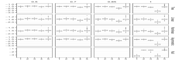
(b) Weibull-I, ISE${}_{\text{out}}$

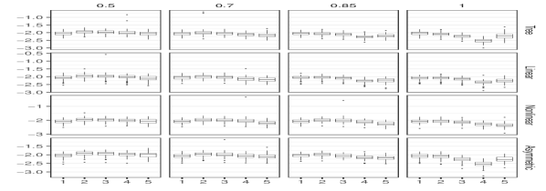
(c) Weibull-D, ISE${}_{\text{in}}$

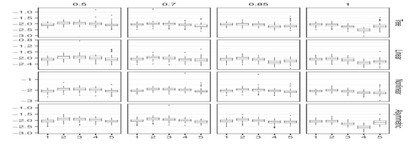
(d) Weibull-D, ISE${}_{\text{out}}$

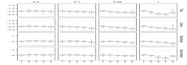
(e) Exponential, ISE${}_{\text{in}}$

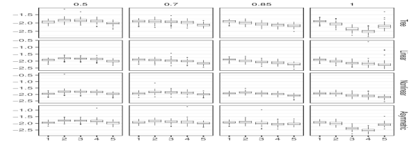
(f) Exponential, ISE${}_{\text{out}}$

Figure 7: Boxplots of integrated squared error (ISE, both in-sample and out-of-sample) on $\log_{10}$ scale, time-varying covariates, N=500, light censoring, Weibull-I, Weibull-D, and Exponential distribution.

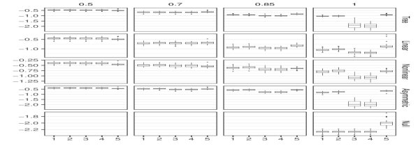
(a) Weibull-I, MSE${}_{y\text{in}}$

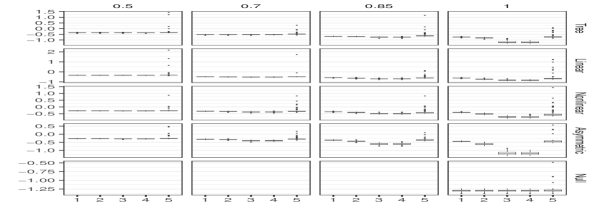
(b) Weibull-I, MSE${}_{y\text{out}}$

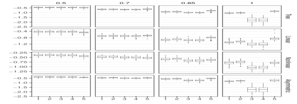
(c) Weibull-D, MSE${}_{y\text{in}}$

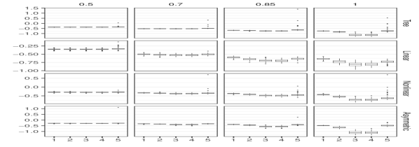
(d) Weibull-D, MSE${}_{y\text{out}}$

(e) Exponential, MSE${}_{y\text{in}}$

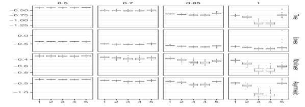
(f) Exponential, MSE${}_{y\text{out}}$

Figure 8: Boxplots of mean squared error (MSE_y, both in-sample and out-of-sample) on $\log_{10}$ scale, time-varying covariates, N=500, light censoring, Weibull-I, Weibull-D, and Exponential distribution.

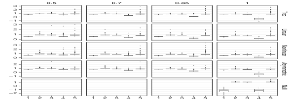
(a) Weibull-I, MSE_b

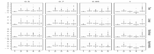
(b) Weibull-D, MSE_b

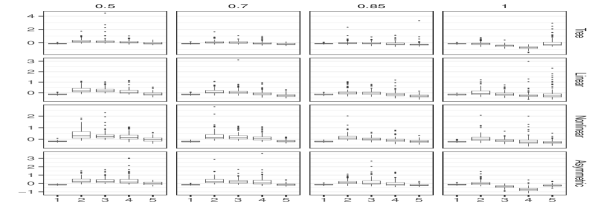
(c) Exponential, MSE_b

Figure 9: Boxplots of mean squared error (MSE_b) of estimated Cox PH slopes on $\log_{10}$ scale, time-varying covariates, N=500, light censoring, Weibull-I, Weibull-D, and Exponential distribution.

Appendix G Comparing various stopping criteria

In this section, we compare three stopping criteria, $\texttt{TS}_{\text{parent}}<\{2.71,3.84,6.63\}$, for Weibull-I distribution and light censoring. We report results for JLCT₄ model in Table 1, i.e. JLCT with time-varying latent class and survival covariates. We use the performance measures described in Section 3.3: ISE${}_{\text{in}}$, ISE${}_{\text{out}}$, MSE${}_{y\text{in}}$, MSE${}_{y\text{out}}$, MSE_b, and Acc_g.

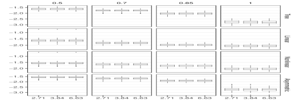
(a) $\log_{10}$ ISE${}_{\text{in}}$

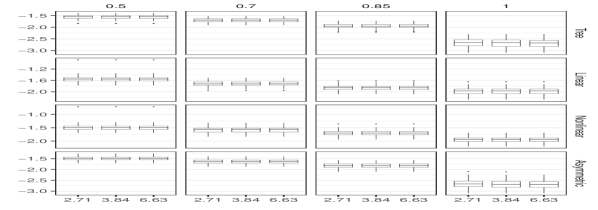
(b) $\log_{10}$ ISE${}_{\text{out}}$

(c) $\log_{10}$ MSEy${}_{\text{in}}$

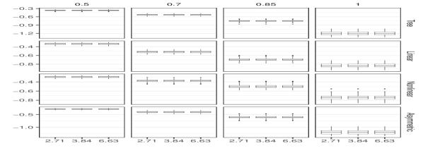
(d) $\log_{10}$ MSEy${}_{\text{out}}$

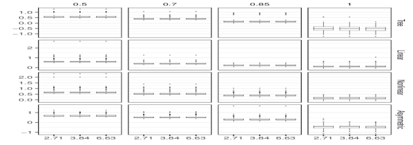
(e) $\log_{10}$ MSEb

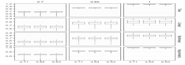
(f) Acc_g

Figure 10: Boxplots of model performance: ISE${}_{\text{in}}$, ISE${}_{\text{out}}$, MSE${}_{y_{\text{in}}}$, MSE${}_{y_{\text{out}}}$, and MSE_b on $\log_{10}$ scale, and Acc_g, for $N=500$, light censoring, and Weibull-I distributions, stopping criteria $\texttt{TS}_{\text{parent}}<\{2.71,3.84,6.63\}$ for JLCT₄ model.

Appendix H Using the R package jlctree

In this section, we demonstrate how to use the R package jlctree to fit JLCT to a simulated data set and to the PAQUID data set. For more details about the jlctree package, please refer to the package manual available at CRAN.

The jlctree package includes an example data set, data_timevar, which is generated under the time-varying setup described in Section D. The call of jlctree to fit JLCT (JLCT₄ in Table 1) to data_timevar is

 

library(jlctree)
data(data_timevar)
tree <- jlctree(survival=Surv(time_L, time_Y, delta)~X3+X4+X5,
            classmb=~X1+X2, fixed=y~X1+X2+X3+X4+X5, random=~1,
            subject=’ID’,data=data_timevar,
            parms=list(maxng=4))

 

Next, we reproduce the results of JLCT on the PAQUID data set. We first convert the original PAQUID data set (contained in the R package lcmm) into left-truncated right-censored (LTRC) format.

 

library(lcmm)
library(NormPsy)
library(data.table)
paquid$normMMSE <- normMMSE(paquid$MMSE)
paquid$age65 <- (paquid$age - 65) / 10
paquidS <- paquid[paquid$agedem > paquid$age_init & paquid$age <= paquid$agedem, ]
paquidS2 <- data.table(paquidS)
paquidS2$age <- paquidS2[,{if(.N==1){age_init}
                          else {c(age_init[1], age[c(1:(.N-1))])}},by=ID][,V1]
temp <- subset(paquidS2, select=c(ID, age_init, agedem, dem, male))
temp <- unique(temp)
data <- tmerge(temp, temp, id=ID, tstart=age_init,
              tstop=agedem, death = event(agedem, dem))
data <- tmerge(data, paquidS2, id=ID, age65 = tdc(age, age65),
               CEP= tdc(age, CEP), normMMSE=tdc(age, normMMSE),
               BVRT=tdc(age, BVRT), IST=tdc(age, IST),
               HIER=tdc(age, HIER), CESD=tdc(age, CESD))
data <- subset(data, !is.na(normMMSE) & !is.na(BVRT)
               & !is.na(IST) & !is.na(HIER) & !is.na(CESD))

  The R code that fits JLCT to the PAQUID dataset using the time-varying covariates, and plots the obtained tree structure as in Figure 3(d), is

 

library(jlctree)
library(rpart.plot)
data$age  <- round(10*data$age65+65)
tree_var <- jlctree(survival=Surv(tstart, tstop, death)~CEP+male+
                BVRT+IST+HIER+CESD+poly(age_init, degree=2, raw=TRUE),
                classmb=~CEP+male+age+BVRT+IST+HIER+CESD,
                fixed=normMMSE~CEP+poly(age65, degree=2, raw=TRUE),
                random=~poly(age65, degree=2, raw=TRUE),
                subject=’id’,data=data,
                parms=list(min.nevents=5, fits=F, fity=F))
rpart.plot(tree_var$tree)

  One can fit JLCT to the PAQUID dataset using the time-invariant covariates by changing the corresponding arguments in the above jlctree call.

References

- [1] Lin H, Turnbull BW, McCulloch CE, Slate EH. Latent class models for joint analysis of longitudinal biomarker and event process data: Application to longitudinal prostate-specific antigen readings and prostate cancer. J Am Stat Assoc;.
- [2] Garre FG, Zwinderman AH, Geskus RB, Sijpkens YW. A joint latent class changepoint model to improve the prediction of time to graft failure. J R Stat Soc A. 2008;171(1):299–308.
- [3] Proust-Lima C, Joly P, Dartigues JF, Jacqmin-Gadda H. Joint modelling of multivariate longitudinal outcomes and a time-to-event: A nonlinear latent class approach. Comput Stat Data Anal. 2009;53(4):1142–1154.
- [4] Perneczky R, Wagenpfeil S, Komossa K, Grimmer T, Diehl J, Kurz A. Mapping scores onto stages: mini-mental state examination and clinical dementia rating. Am J Geriatr Psychiatry. 2006;14(2):139–144.
- [5] Longini Jr IM, Clark WS, Byers RH, Ward JW, Darrow WW, Lemp GF, et al. Statistical analysis of the stages of HIV infection using a Markov model. Stat Med. 1989;8(7):831–843.
- [6] Dicker R, Coronado F, Koo D, Parrish RG. Principles of epidemiology in public health practice. US Department of Health and Human Services. 2012;https://www.cdc.gov/csels/dsepd/ss1978/SS1978.pdf. Accessed 17 June 2019.
- [7] Antonelli-Incalzi R, Imperiale C, Bellia V, Catalano F, Scichilone N, Pistelli R, et al. Do GOLD stages of COPD severity really correspond to differences in health status? Eur Respir J. 2003;22(3):444–449.
- [8] Hajiro T, Nishimura K, Tsukino M, Ikeda A, Oga T. Stages of disease severity and factors that affect the health status of patients with chronic obstructive pulmonary disease. Respir Med. 2000;94(9):841–846.
- [9] Proust-Lima C, Taylor JM. Development and validation of a dynamic prognostic tool for prostate cancer recurrence using repeated measures of posttreatment PSA: A joint modeling approach. Biostatistics. 2009;10(3):535–549.
- [10] Proust-Lima C, Philipps V, Liquet B. Estimation of Extended Mixed Models Using Latent Classes and Latent Processes: The R Package lcmm. J Stat Softw. 2017;78(2):1–56.
- [11] Zhang N, Simonoff JS. The Potential for Nonparametric Joint Latent Class Modeling of Longitudinal and Time-to-Event Data. In: LaRocca M, Liseo B, Salmaso L, editors. Nonparametric Statistics — 4th ISNPS, Salerno, Italy, June 2018. Springer; 2021. p. to appear.
- [12] Breiman L, Friedman JH, Olshen RA, Stone CJ. Classification and Regression Trees. Monterey, CA, USA: Wadsworth and Brooks; 1984.
- [13] Hastie T, Tibshirani R, Friedman J. The Elements of Statistical Learning. New York, NY, USA: Springer New York Inc.; 2001.
- [14] Cox DR. Regression Models and Life-Tables. J R Stat Soc B. 1972;34(2):187–220.
- [15] Andersen PK, Gill RD. Cox’s regression model for counting processes: A large sample study. Ann Stat. 1982;10(4):1100–1120.
- [16] Fu W, Simonoff JS. Survival trees for left-truncated and right-censored data, with application to time-varying covariate data. Biostatistics. 2017;18(2):352–369.
- [17] Laird NM, Ware JH. Random-effects models for longitudinal data. Biometrics. 1982;38(4):963–974.
- [18] Hothorn T, Hornik K, Zeileis A. Unbiased recursive partitioning: A conditional inference framework. J Comput Graph Stat. 2006;15(3):651–674.
- [19] Proust-Lima C, Philipps V, Diakite A, Liquet B. lcmm: Extended Mixed Models Using Latent Classes and Latent Processes; 2018. R package version: 1.7.9. Available from: https://cran.r-project.org/package=lcmm.
- [20] Letenneur L, Commenges D, Dartigues JF, Barberger-Gateau P. Incidence of dementia and Alzheimer’s disease in elderly community residents of south-western France. Int J Epidemiol. 1994;23(6):1256–1261.
- [21] Wulfsohn MS, Tsiatis AA. A joint model for survival and longitudinal data measured with error. Biometrics. 1997;53(1):330–339.
- [22] Henderson R, Diggle P, Dobson A. Joint modelling of longitudinal measurements and event time data. Biostatistics. 2000;1(4):465–480.
- [23] Tsiatis AA, Davidian M. Joint modeling of longitudinal and time-to-event data: An overview. Stat Sin. 2004;14(3):809–834.
- [24] Rizopoulos D. JM: An R package for the joint modelling of longitudinal and time-to-event data. J Stat Softw. 2010;35(9):1–33.
- [25] Blanche P, Proust-Lima C, Loubère L, Berr C, Dartigues JF, Jacqmin-Gadda H. Quantifying and comparing dynamic predictive accuracy of joint models for longitudinal marker and time-to-event in presence of censoring and competing risks. Biometrics. 2015;71(1):102–113.
- [26] Graf E, Schmoor C, Sauerbrei W, Schumacher M. Assessment and comparison of prognostic classification schemes for survival data. Stat Med. 1999;18(17-18):2529–2545.
- [27] Pradier C, Sakarovitch C, Le Duff F, Layese R, Metelkina A, Anthony S, et al. The Mini Mental State Examination at the Time of Alzheimer’s Disease and Related Disorders Diagnosis, According to Age, Education, Gender and Place of Residence: A Cross-Sectional Study among the French National Alzheimer Database. PLOS ONE. 2014 08;9(8):1–8.
- [28] Tsoi KK, Chan JY, Hirai HW, Wong SY, Kwok TC. Cognitive tests to detect dementia: a systematic review and meta-analysis. JAMA Intern Med. 2015;175(9):1450–1458.
- [29] Liu Y, Liu L, Zhou J. Joint latent class model of survival and longitudinal data: An application to CPCRA study. Comput Stat Data Anal. 2015;91:40–50.
- [30] Proust-Lima C, Séne M, Taylor JM, Jacqmin-Gadda H. Joint latent class models for longitudinal and time-to-event data: A review. Stat Methods Med Res. 2014;23(1):74–90.
- [31] Crowley J, Hu M. Covariance analysis of heart transplant survival data. J Am Stat Assoc;.
- [32] Tsiatis AA, Degruttola V, Wulfsohn MS. Modeling the relationship of survival to longitudinal data measured with error. Applications to survival and CD4 counts in patients with AIDS. J Am Stat Assoc;.
- [33] Dekker FW, De Mutsert R, Van Dijk PC, Zoccali C, Jager KJ. Survival analysis: Time-dependent effects and time-varying risk factors. Kidney Int. 2008;74(8):994–997.
- [34] Kovesdy CP, Anderson JE, Kalantar-Zadeh K. Paradoxical association between body mass index and mortality in men with CKD not yet on dialysis. Am J Kidney Dis. 2007;49(5):581–591.
- [35] Jongerden IP, Speelberg B, Satizábal CL, Buiting AG, Leverstein-van Hall MA, Kesecioglu J, et al. The role of systemic antibiotics in acquiring respiratory tract colonization with gram-negative bacteria in intensive care patients: A nested cohort study. Crit Care Med. 2015;43(4):774–780.
- [36] Munoz-Price LS, Frencken JF, Tarima S, Bonten M. Handling time-dependent variables: Antibiotics and antibiotic resistance. Clin Infect Dis. 2016;62(12):1558–1563.
- [37] Therneau TM. A Package for Survival Analysis in S; 2015. Version 2.38. Available from: https://CRAN.R-project.org/package=survival.
- [38] Therneau TM, Grambsch PM. Modeling Survival Data: Extending the Cox Model. New York: Springer; 2000.
- [39] Bates D, Mächler M, Bolker B, Walker S. Fitting Linear Mixed-Effects Models Using lme4. J Stat Softw. 2015;67(1):1–48.