Quantum aspects of self-interacting fields around cosmic strings

Abstract

We study the quantum effect of self-interacting fields in the classical background of conical space, i.e. around, a cosmic string with infinitesimal width. The renormalized value of $\langle\phi^{2}\rangle$ and energy-momentum tensor in the presence of cosmic strings are calculated in the self-interacting scalar field theory. The amount of condensation is also estimated in the case of the Dirac Lagrangian with the four-fermion interaction. The physical implications of the above analyses are discussed.

1 Introduction

The recent enthusiasm for cosmic strings [1] comes from the possibility that loops of strings provide the seeds for galaxies. The cosmic strings which have large energy density give seeds for galaxies. However, the dimensionless combination $G\mu$, where $G$ is the Newton constant and $\mu$ stands for the energy density of the string per unit length, must not be too large to avoid conflict with astronomical observation. The most stringent limit is derived from observation of the microwave background [2]. A network of cosmic strings moving at a relativistic speed may generate a characteristic pattern of anisotropy in the temperature of the radiation. The upper limit of anisotropy places constraints on $G\mu$. According to the result, it is concluded that ‘massive’ strings which have $G\mu$ much larger than $5\times 10^{-6}$ could not exist in the early universe.

Even in the static case, it is known that the gravitational field around an infinitely stretching straight string has a peculiar property. An idealized static string, which has an infinitesimal thickness, cannot create a Newtonian gravitational potential around it [1, 3]. Indeed, beside the singularity on the string, the spacetime around the string has vanishing curvature everywhere. The global structure of the space is, however, non-trivial as many authors advocated.

Suppose the idealized cosmic string lies on the $z$-axis. The metric of the cylindrically symmetric space can be written [3]

$$ds^{2}=-dt^{2}+dr^{2}+(r^{2}/\nu^{2})d\theta^{2}+dz^{2}\,,$$ (1)

where $\nu^{-1}=1-4G\mu<1$ and $r$ and $\theta$ are the polar coordinates of the $xy$ plane. If we use a new coordinate

$$\tilde{\theta}\equiv\theta/\nu\,,$$ (2)

we find that the metric reduces to the flat Minkowski spacetime except for the deficit in the azimuthal angle because $\tilde{\theta}$ takes the value from zero to $2\pi/\nu$. In this interpretation, it can be said that the space has a conical singularity at the location of the idealized cosmic string.

Several authors have studied the quantum field theory around the conical space [4, 5, 6, 7, 8, 9]. In many cases, quantum effects are solved exactly owing to the local flatness of the spacetime. Furthermore, the quantum aspects around the string attract much attention as an example of illustrating the importance of global topology in field theory.

From the physical and astrophysical viewpoint, we must carefully take the quantum effect around string, because it may be a menace to the existence of the string itself. The gravitational effect is independent of the detail of the internal structure of cosmic string, i.e., the symmetry breaking which produces the topological defects. Therefore, for example, if the energy density induced from the quantum polarization becomes enormous, catastrophic increase of the energy density of the string may occur and at least static straight string-like objects no longer exist.

According to several authors, so far no terrible effect can be found due to the free quantum fields around the string. In this paper we analyse the quantum effects of interacting field theories around the string. The interaction of fields may enhance or suppress the amount of the quantum-effect of free fields. We will clarify this point and discuss its implications.

Although we treat an idealized string in the present paper, an ‘actual’ string is expected to be made of self-interacting Higgs-like field. Thus symmetry breaking near the string is an important subject to study. A study along this line has been made by Russell and Toms [9]. They did not evaluate physical quantities such as energy density in free space around the string. We follow the essence of their method in treating interaction consistently, to calculate the renormalized value of $\langle\phi^{2}\rangle$ and the energy-momentum tensor.

In section 2 we calculate the renormalized value of $\langle\phi^{2}\rangle$ and the energy-momentum tensor for a massive scalar. The derivation includes not only a review of the technique to get the analytic form for the Green function but also detailed estimations of $\langle\phi^{2}\rangle$ and the energy-momentum tensor which have not been exhibited explicitly.

In section 3 we consider the self-interacting massless scalar field. The effect of interaction is treated self-consistently. The renormalized $\langle\phi^{2}\rangle$ and the energy-momentum tensor are calculated.

In section 4 we estimate the amount of condensation of fermions in a self-interacting model such as the Nambu-Jona-Lasinio model [10, 11].

Section 5 is devoted to a summary and discussion.

2 The calculation of vacuum fluctuations in massive scalar field theory in the conical space

In this section we demonstrate the calculation of quantum fluctuations of a massive free scalar field. We first determine the two-point function of the scalar field, because the renormalized value of $\langle\phi^{2}\rangle$ and the energy-momentum tensor due to vacuum polarization can be derived from the two-point function and a regularization procedure.

Several authors have developed methods of computing the two-point functions [4, 5, 6, 7, 8, 9]. We follow the method given by Smith [8], for it seems very simple and applicable.

In his method, we must first solve the normal mode of the wavefunction in the background of conical space described as (1). If we write the mode function as

$$f(r,\theta,z,t)=R(r)e^{im\theta}e^{ikz}e^{-i\omega t}\,,$$ (3)

we find that the function $R(r)$ obeys the Bessel equation:

$$\left(\frac{1}{r}\frac{d}{dr}r\frac{d}{dr}+(\omega^{2}-k^{2}-M^{2})-\frac{\nu^{2}m^{2}}{r^{2}}\right)R(r)=0\,,$$ (4)

where $M$ is the mass of the scalar. Here we follow the notation of Smith [8], except for $\nu$ which stands for his $p$ and the definition of $O$. He managed to sum up the bilinear of the mode functions on their ‘labels’; especially for the radial function the summation is forced to be an integration. By the same prescription as his, we obtain

$$G_{\nu}(x,x^{\prime})\equiv\langle 0|\phi(x)\phi(x^{\prime})|0\rangle$$

$$=\frac{\nu}{4\pi^{2}}\sum_{m=-\infty}^{\infty}e^{im(\theta-\theta^{\prime})}\int_{0}^{\infty}dK\,K\,J_{\nu|m|}(Kr)J_{\nu|m|}(Kr^{\prime})K_{0}[(K^{2}+M^{2})^{1/2}\zeta]\,,$$ (5)

where $J_{p}(x)$ is a Bessel function, $K_{p}(x)$ is a modified Bessel function of the second kind and $\zeta^{2}=(z-z^{\prime})^{2}-(t-t^{\prime})^{2}$. If $M=0$ is substituted, then it recovers the result of Smith for a massless scalar [8].

We can rewrite $K_{0}[(K^{2}+M^{2})^{1/2}\zeta]$ in an integral representation [12]:

$$K_{0}[(K^{2}+M^{2})^{1/2}\zeta]=\frac{1}{2}\int_{0}^{\infty}\frac{dt}{t}\exp\left(-t-\frac{(K^{2}+M^{2})\zeta^{2}}{4t}\right)\,.$$ (6)

Using this representation, the integration with respect to $K$ can be done. Then we obtain [12]

$$G_{\nu}=\frac{\nu}{4\pi^{2}\zeta^{2}}\sum_{m=-\infty}^{\infty}e^{im(\theta-\theta^{\prime})}\int_{0}^{\infty}dt\,I_{\nu|m|}\left(\frac{2rr^{\prime}}{\zeta^{2}}t\right)\exp\left(-\frac{r^{2}+{r^{\prime}}^{2}+\zeta^{2}}{\zeta^{2}}t-\frac{M^{2}\zeta^{2}}{4t}\right)\,,$$ (7)

where $I_{\mu}(x)$ is a modified Bessel function of the first kind.

To compare this with the result of Linet [5], we now use the integral form of $I_{\mu}(z)$ [12]:

$$I_{\mu}(z)=\frac{1}{\pi}\int_{0}^{\pi}e^{z\cos\theta}\cos\mu\theta\,d\theta-\frac{\sin\mu\pi}{\pi}\int_{0}^{\infty}e^{-z\cosh x-\mu x}dx\,.$$ (8)

With the aid of the following identity

$$\frac{1}{2\pi}\sum_{m=-\infty}^{\infty}e^{im\psi}\cos\nu|m|\theta=\frac{1}{2\nu}\left[\delta\left(\theta-\frac{\psi}{\nu}\right)+\delta\left(\theta+\frac{\psi}{\nu}\right)\right]\,,$$ (9)

we can carry out the summation on $m$ and we get:

$$G_{\nu}=\frac{M}{4\pi^{2}\{r^{2}+{r^{\prime}}^{2}-2rr^{\prime}\cos(\varphi/\nu)+\zeta^{2}\}^{1/2}}$$

$$\times K_{1}(M\{r^{2}+{r^{\prime}}^{2}-2rr^{\prime}\cos(\varphi/\nu)+\zeta^{2}\}^{1/2})$$

$$+\frac{M\nu}{8\pi^{3}}\int_{0}^{\infty}\frac{K_{1}(M\{r^{2}+{r^{\prime}}^{2}+2rr^{\prime}\cosh t+\zeta^{2}\}^{1/2})}{(r^{2}+{r^{\prime}}^{2}+2rr^{\prime}\cosh t+\zeta^{2})^{1/2}}$$

$$\times\left(\frac{\sin(\varphi-\nu\pi)}{\cosh\nu t-\cos(\varphi-\nu\pi)}-\frac{\sin(\varphi+\nu\pi)}{\cosh\nu t-\cos(\varphi+\nu\pi)}\right)dt\,,$$ (10)

where $\varphi\equiv\theta-\theta^{\prime}$.

This result coincides with that computed by Linet [5]. The last form may be accomplished by any other method, and even in an easier way.

For scalar bosons, it is well known that the vacuum expectation value of the energy-momentum tensor and $\langle\phi^{2}\rangle$ can be calculated from the Green function. We can obtain them for the massive scalar case using the Green function (10).

$\langle\phi^{2}\rangle$ is the coincidence limit of the renormalized Green function:

$$\langle\phi^{2}\rangle=\lim_{x^{\prime}\rightarrow x}G_{\nu~{}ren}(x^{\prime},x)\,,$$ (11)

where $G_{\nu~{}ren}=G_{\nu}-G_{1}$.

Because of the identical nature of divergences in the coincidence limit in both a cosmic string and the Minkowski background, the subtraction of the same quantity in Minkowski space assures a finite and meaningful renormalization scheme.

Similarly the energy-momentum tensor is given by

$$\langle T_{\lambda}^{\mu}\rangle=\lim_{x^{\prime}\rightarrow x}[T_{\lambda}^{\mu}(\nu;x^{\prime},x)-T_{\lambda}^{\mu}(1;x^{\prime},x)]\,,$$ (12)

where

$$T_{\lambda}^{\mu}(\nu;x^{\prime},x)$$

$$=\left\{\left[(1-2\xi)\nabla^{\mu}\nabla_{\lambda^{\prime}}-\left(\frac{1}{2}-2\xi\right)\delta_{\lambda}^{\mu}\nabla^{\rho}\nabla_{\rho^{\prime}}-2\xi\nabla^{\mu}\nabla_{\lambda}\right.\right.$$

$$\qquad\qquad\qquad\qquad\qquad\left.\left.+M^{2}\left(2\xi-\frac{1}{2}\right)\delta_{\lambda}^{\mu}\right]G_{\nu}(x,x^{\prime})\right\}$$ (13)

and $\nabla_{\mu}~{}(\nabla_{\mu^{\prime}})$ denotes the covariant derivative with respect to the coordinates $x~{}(x^{\prime})$. $\xi$ is the coupling to the scalar curvature. Here we take the conformal coupling, $\xi=1/6$, in the calculation of the energy-momentum tensor, for simplicity.

The exact expression of $\langle\phi^{2}\rangle$ for a massive scalar field is very lengthy, but the estimation in the limiting cases can be simply carried out.

For $Mr\ll 1$, we obtain

$$\langle\phi^{2}\rangle=\frac{\nu^{2}-1}{48\pi^{2}r^{2}}\,,$$ (14)

$$\langle T_{\lambda}^{\mu}\rangle=\frac{\nu^{4}-1}{1440\pi^{2}r^{4}}\mbox{diag.}(1,1,-3,1)\,.$$ (15)

These are the same results as a massless scalar case.

For $Mr\gg 1$, we get

$$\langle\phi^{2}\rangle=\frac{\nu\tan(\pi(\nu-1)/2)}{8\pi^{2}r^{2}}e^{-2Mr}\,,$$ (16)

$$\langle T_{\lambda}^{\mu}\rangle=\frac{\nu\tan(\pi(\nu-1)/2)M^{2}}{24\pi^{2}r^{2}}\mbox{diag.}(-1,0,-1,-1)\,,$$ (17)

for $\xi=1/6$ at the leading order in the expansion with respect to the powers of $(Mr)^{-1}$. We find that exponential damping appears in these quantities, which is coincident with a naive expectation.

Now the warming-up is over; we will try to consider the inclusion of self-interaction of bosons in the next section.

3 Inclusion of self-interaction of scalars

In this section we consider a massless scalar field theory with a quartic self-interaction. The Lagrangian density for the theory is

$$L=\frac{1}{2}\nabla_{\mu}\phi\nabla^{\mu}\phi+\frac{1}{2}\xi R\phi^{2}+\frac{\lambda}{4!}\phi^{4}\,,$$ (18)

where $\lambda$ is a dimensionless coupling.

One of the reasons for our consideration of the massless case is just for simplicity. Another reason is as follows; as we have seen in the last section, the quantum effects are expected to fade out exponentially with distance from the string. Thus only in the region $Mr\ll 1$ may the interaction play an important role in the calculation of the physical quantities.

The interacting field around the cosmic string has been considered by Russell and Toms [9]. They have taken special care of the boundary conditions and the instability of each mode of the wavefunction.

In this paper, our aim is to calculate $\langle\phi^{2}\rangle$ and the energy-momentum tensor explicitly in the presence of a quartic interaction without any boundary condition at a finite distance. To this end, we treat the effect of interaction with an iterative method.

We expect that the vacuum value of $\langle\phi^{2}\rangle$ is expressed as

$$\langle\phi^{2}\rangle=\frac{\alpha}{r^{2}}\,,$$ (19)

where $\alpha$ is a dimensionless constant, because there is no dimensional coupling. Now the problem is to obtain the value of $\alpha$. We try to determine $\langle\phi^{2}\rangle$ in the following self-consistent way.

The equation of motion according to the Lagrangian (18) is

$$-\nabla_{\mu}\nabla^{\mu}\phi+\xi R\phi+\frac{\lambda}{3!}\phi^{3}=0\,.$$ (20)

The coupling to the curvature is irrelevant to the Green function at this time, since the spacetime around the cosmic string is locally flat everywhere except for just on the string.

Here we apply a ‘Hartree-like’ approximation to the equation (20); we substitute

$$\phi^{3}\approx 3\langle\phi^{2}\rangle\phi\,.$$ (21)

Then we can construct the Green function by following the same method in the previous section. Now the equation of motion is linearized by substitution of (21) and (19); thus the radial function $R(r)$, similarly defined by (3), satisfies

$$\left(\frac{1}{r}\frac{d}{dr}r\frac{d}{dr}+(\omega^{2}-k^{2})-\frac{\nu^{2}m^{2}+\alpha^{\prime}}{r^{2}}\right)R(r)=0\,,$$ (22)

where $\alpha^{\prime}\equiv\frac{1}{2}\lambda\alpha$.

Consequently, we obtain the integral form for the Green function with yet undetermined $\alpha^{\prime}$ in this case:

$$G_{\nu}(x,x^{\prime};\alpha^{\prime})=\frac{\nu}{4\pi^{2}}\sum_{m=-\infty}^{\infty}e^{im(\theta-\theta^{\prime})}$$

$$\cdot\int_{0}^{\infty}dK\,K\,J_{(\nu^{2}m^{2}+\alpha^{\prime})^{1/2}}(Kr)J_{(\nu^{2}m^{2}+\alpha^{\prime})^{1/2}}(Kr^{\prime})K_{0}[(K^{2}+M^{2})^{1/2}\zeta]\,.$$ (23)

Now our plan to estimate $\langle\phi^{2}\rangle$ and the energy-momentum in this case is as follows. The derivation $\langle\phi^{2}\rangle(\alpha^{\prime})$ from the renormalized Green function can be quite parallel to that explained in section 2. The renormalized Green function is defined as $G_{\nu~{}ren}=G_{\nu}-G_{1}$. Then we first solve the self-consistent equation on $\langle\phi^{2}\rangle$

$$\frac{\alpha^{\prime}}{r^{2}}=\frac{1}{2}\lambda\langle\phi^{2}\rangle(\alpha^{\prime})\,.$$ (24)

Next we substitute the value of a’ into the expression for the energy-momentum tensor. This technique is rather like the large $N$ approximation [13], although $N=1$ in the present case.

Let us return to the actual calculations. For the massless case, the integration with respect to the variable $K$ can be carried out first and yields

$$G_{\nu}(x,x^{\prime};\alpha^{\prime})=\frac{\nu}{8\pi^{2}rr^{\prime}\sinh u}\sum_{m=-\infty}^{\infty}\exp[im(\theta-\theta^{\prime})]\exp[-(\nu^{2}m^{2}+\alpha^{\prime})^{1/2}u]\,.$$ (25)

where $\cosh u\equiv\{r^{2}+{r^{\prime}}^{2}+\zeta^{2}\}/2rr^{\prime}=\{r^{2}+{r^{\prime}}^{2}+(z-z^{\prime})^{2}-(t-t^{\prime})^{2}\}/2rr^{\prime}$. One can see that this reduces to the well known result [4, 5, 6, 7, 8, 9] if we let $\alpha^{\prime}$ go to zero.

Taking the coincidence limit of the renormalized Green function as (11), we can reduce (24) for self-consistency to

$$\frac{\sqrt{\alpha^{\prime}}}{\lambda}=\frac{1}{8\pi^{3}}\sum_{n=1}^{\infty}\frac{1}{n}\left[\nu K_{1}\left(\frac{2\pi\sqrt{\alpha^{\prime}}n}{\nu}\right)-K_{1}\left({2\pi\sqrt{\alpha^{\prime}}n}\right)\right]\,.$$ (26)

This equation is solved numerically. The result is shown in figure 1, for $\nu=1+10^{0}$, $1+10^{-2}$ and $1+10^{-4}$. In this figure, we exhibit $F_{1}\equiv 48\pi^{2}r^{2}\langle\phi^{2}\rangle$ as the result of the solution of (26).

For very small $\lambda$

$$F_{1}\approx\nu^{2}-1\,,$$ (27)

whereas for relatively large $\lambda$, $F_{1}$ decreases in a moderate way.

The energy-momentum tensor in the present scheme can be written as

$$\langle T_{\lambda}^{\mu}(\alpha^{\prime}(\lambda))\rangle=\lim_{x^{\prime}\rightarrow x}[T_{\lambda}^{\mu}(\nu;\alpha^{\prime})-T_{\lambda}^{\mu}(1;\alpha^{\prime})]\,,$$ (28)

$$T_{\lambda}^{\mu}(\nu;\alpha^{\prime})$$

$$=\left\{\left[(1-2\xi)\nabla^{\mu}\nabla_{\lambda^{\prime}}-\left(\frac{1}{2}-2\xi\right)\delta_{\lambda}^{\mu}\nabla^{\rho}\nabla_{\rho^{\prime}}-2\xi\nabla^{\mu}\nabla_{\lambda}\right.\right.$$

$$\qquad\qquad\qquad\qquad\qquad\left.\left.+\frac{1}{2}\left(2\xi-\frac{1}{4}\right)\lambda\langle\phi^{2}\rangle\delta_{\lambda}^{\mu}\right]G_{\nu}(x,x^{\prime};\alpha^{\prime})\right\}\,,$$ (29)

where a ‘Gaussian’ approximation has been adopted. This treatment is compatible with the previous Hartree approximation. The value for a’ is to be taken as that we obtained as a solution of (26).

Some manipulations lead to the following result;

$$\langle T_{\lambda}^{\mu}\rangle=\frac{1}{1440\pi^{2}r^{4}}F_{3}\mbox{diag.}(1,1,-3,1)+\frac{1}{24\pi^{2}r^{4}}F_{1}\mbox{diag.}(2,-1,3,2)\,,$$ (30)

where

$$F_{3}=90\sum_{n=1}^{\infty}\frac{(\alpha^{\prime})^{3/2}}{\pi n}\left[\nu K_{3}\left(\frac{2\pi\sqrt{\alpha^{\prime}}n}{\nu}\right)-K_{3}\left({2\pi\sqrt{\alpha^{\prime}}n}\right)\right]\,,$$ (31)

and

$$F_{1}=12\sum_{n=1}^{\infty}\frac{\sqrt{\alpha^{\prime}}}{\pi n}\left[\nu K_{1}\left(\frac{2\pi\sqrt{\alpha^{\prime}}n}{\nu}\right)-K_{1}\left({2\pi\sqrt{\alpha^{\prime}}n}\right)\right]\,.$$ (32)

In these expressions, $\alpha^{\prime}$ is recognized as the solution of (26). Consequently, $F_{1}$ (32) is the same as the previous definition.

Note that the values of both $F_{3}$ and $F_{1}$ for finite $\alpha^{\prime}$ are less than those for $\alpha^{\prime}\rightarrow 0$, that is, the limit of $\lambda=0$.

In figures 1 and 2, numerical values for the functions $F_{1}$ and $F_{3}$ are plotted against $\lambda$, respectively.

To summarize this section, we obtain the numerical value of the renormalized value for $\langle\phi^{2}\rangle$ and the components of the energy-momentum tensor in the interacting scalar model with a quartic coupling. We find $r^{2}\langle\phi^{2}\rangle$ becomes smaller for a finite $\lambda$. The decrease is, however, a moderate one for each case when the parameter $\nu$ takes a realistic value such that $\nu-1\approx 10^{-6}$. The absolute values of the components of the energy-momentum tensor always become smaller when $\lambda\neq 0$ and for any $\nu$. Thus no catastrophic characteristics are found in the interacting boson theory, at least in the approximation scheme.

In the next section, we will examine the self-interacting fermionic fields around the string.

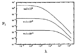
Figure 1: $F_{1}$ plotted against the self-coupling $\lambda$ (see text).

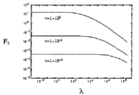
Figure 2: $F_{3}$ plotted against $\lambda$ (see text).

4 Fermion condensate in four fermion interaction theory near the cosmic string

In this section we investigate an interacting-fermion model. We consider a four-fermion interacting model in four dimensions. We assume that, as a physical situation, the thickness of the string is comparable with the inverse of the scale A at which some fundamental interaction between fermions is expected. Then we treat the string thickness as infinitesimal for simplicity, and again use the metric defined in section 1.

The Lagrangian density under consideration is

$$L=i\bar{\psi^{a}}\gamma^{\mu}\nabla_{\mu}\psi^{a}+G(\bar{\psi^{a}}\psi^{a})^{2}\,,$$ (33)

where the suffix $a$ denotes the ‘colour’ or species, of the fermions, which is taken as $N$, and the coupling $G$ is of order $\Lambda^{-2}$. To see whether the dynamical generation of the fermion mass occurs or not, we examine the following gap equation;

$$M=-\frac{1}{2}G\langle\bar{\psi}\psi\rangle\,,$$ (34)

where $M$ is the mass of the fermion field, and $\langle\bar{\psi}\psi\rangle$ is recognized as

$$\langle\bar{\psi}\psi\rangle=N\lim_{x^{\prime}\rightarrow x}{\rm Tr~{}}S(x,x^{\prime};M)\,,$$ (35)

where $S$ is the propagator (or Green function) of a single fermion field with mass$=M$.

In the conical background space, we replace the fermion propagator with $S_{\nu}$. For a massless case, the fermion Green function in the conical space is explicitly obtained in [6]. The extension to the massive case is a tedious but workable task.

In the present paper we will estimate the right-hand side of the gap equation at the leading order. We note that the large contribution arises from the region where $Mr\ll 1$, as in the boson case (in section 2). Further, we assume the spatial variation of the mass of the fermion is gentle and small.

At the spatial infinity from the origin, the gap equation must be the same as the flat spacetime;

$$M_{\infty}=\frac{GN}{8\pi^{2}}M_{\infty}\left(\Lambda^{2}-M_{\infty}^{2}\ln\frac{\Lambda^{2}}{M_{\infty}^{2}}\right)\,,$$ (36)

where $\Lambda$ is the momentum cut-off. On the other hand, at a finite distance from the string, we have

$$M_{r}=\frac{GN}{8\pi^{2}}M_{r}\left(\Lambda^{2}-M_{r}^{2}\ln\frac{\Lambda^{2}}{M_{r}^{2}}-\Delta(r,M_{r})\right)\,,$$ (37)

where $M_{r}$ is the mass of the fermion field at the radial distance $r$ from the string and $\Delta(r,M_{r})$ is defined as

$$\Delta(r,M_{r})=\frac{4\pi^{2}}{M_{r}}\lim_{x^{\prime}\rightarrow x}{\rm Tr~{}}S_{\nu~{}ren}(x,x^{\prime};M_{r})\,,$$ (38)

where $S_{\nu~{}ren}(x,x^{\prime};M_{r})$ is the renormalized massive fermion propagator in the conical space. The assumption that the variation of $M_{r}$ is slow has been used in (36).

From (36) and (37), the gap equation (37) has a non-trivial solution only if

$$\Delta<M_{\infty}\ln(\Lambda^{2}/M_{\infty}^{2})$$ (39)

is satisfied.

We calculate $\Delta$ in the limit $M_{r}r\ll 1$; otherwise, the vacuum polarization effect is expected to be suppressed exponentially. The calculation can simply be done by only use of the massless propagator of a fermion. The result is

$$\Delta=\frac{4\pi^{2}}{M_{r}}\frac{(\nu^{2}-1)M_{r}}{24\pi^{2}r^{2}}=\frac{\nu^{2}-1}{6r^{2}}\,.$$ (40)

Then we find that the dynamical mass generation is absent in the vicinity of the string. The radius of the region is

$$r<r_{c}=\left(\frac{\nu^{2}-1}{6M_{\infty}^{2}\ln(\Lambda^{2}/M_{\infty}^{2})}\right)^{1/2}\,.$$ (41)

In this region, $Mr\ll 1$ is satisfied and the right-hand side of (41) is sufficiently large compared to $1/\Lambda$. For instance, if we take $\nu=1+10^{-6}$, $\Lambda=10^{15}$GeV and $M=100$GeV, and then $\Lambda r_{c}\simeq 10^{9}$. Even if the four-fermion interaction is not a ‘fundamental’ interaction, but induced from the exchange of bosons whose masses are of order of $\Lambda$, the conclusion does not change because $\Lambda r_{c}\gg 1$. Thus our assumption in the approximation scheme is adequate.

Note that the present phenomenon is only due to the spacetime structure. Although the thickness of the symmetry restoration is very small, the length scale along the string may be macroscopic.

5 Summary and discussion

In this paper, we have investigated quantum aspects of self-interacting fields around the idealized string. For the self-interacting scalar field theory, the vacuum value $\langle\phi^{2}\rangle$ turns out to become small when self-coupling exists. The vacuum stress tensor is reduced in the presence of the self-interaction. Thus no drastic effect on the very existence of the string-like object is expected.

On the other hand, in the self-interacting fermion theory, the mass generation of the fermion does not occur very near the string. This leads to the restoration of the symmetry in some models [11]. In such models [11] the condensation of gauge fields may take place. The thickness of the region is very tiny, but the length scale can be macroscopic along the cosmic string. The effect may have some importance in the very early universe if it is applied to some complicated theories. The detailed analyses including numerical results will be reported in future works.

The back-reaction involving the gravitational field is worth studying. At the same time, the study of quantum effects of the electromagnetic fields of superconducting cosmic string [14] is very interesting when charged matter fields coupled with each other are taken into account. We hope to report these studies.

Note added in proof

Since submission of this paper, we have been informed of the papers [15], which treat interacting fields around a cosmic string.

We are very grateful to the referees for helpful comments and information.

References

- [1] A. Vilenkin, Phys. Rep. 121 (1985) 263.
- [2] D. P. Bennett and F. R. Bouchet, Phys. Rev. D43 (1991) 2733.
- [3] A. Vilenkin, Phys. Rev. D23 (1981) 852. J. R. Gott, Astrophys. J. 288 (1985) 411.
- [4] J. S. Dowker, Phys. Rev. D36 (1987) 3742. J. S. Dowker, The Formation and Evolution of Cosmic Strings ed G. Gibbons, S. Hawking and T. Vachaspati (Cambridge: Cambridge University Press, 1989) p. 251.
- [5] B. Linet, Phys. Rev. D35 (1987) 536.
- [6] V. P. Frolov and E. M. Serebriany, Phys. Rev. D35 (1987) 3779.
- [7] A. Sarmiento and S. Hacyan, Phys. Rev. D38 (1988) 1331.
- [8] A. G. Smith, The Formation and Evolution of Cosmic Strings ed G. Gibbons, S. Hawking and T. Vachaspati (Cambridge: Cambridge University Press, 1989) p. 263.
- [9] I. H. Russell and D. J. Toms, Class. Quantum Grav. 6 (1989) 1343.
- [10] Y. Nambu and G. Jona-Lasinio, Phys. Rev. 122 (1961) 345.
- [11] W. A. Bardeen, C. T. Hill and M. Lindner, Phys. Rev. D41 (1990) 1647.
- [12] S. Gradshteyn and I. M. Ryzhik, Tables of Integrals, Series and Products (New York: Academic, 1965)
- [13] S. Coleman, R. Jackiw and H. D. Politzer, Phys. Rev. D10 (1974) 2491.
- [14] E. Witten, Nucl. Phys. B249 (1985) 557.
- [15] D. Harari and V. Skarzhinsky, Phys. Lett. B240 (1990) 322. J. Audretsch and A. Economou, 1991 Phys. Rev. D44 (1991) 980.