Abstract

There is a special class of so-called block-scalable initial states of the sender whose transfer to the receiver through the spin chain results in multiplying their MQ-coherence matrices by scalar factors (block-scaled receiver’s states). We study the entanglement in block-scalable and block-scaled states and show that, generically, the entanglement in block scaled states is less than the entanglement in the corresponding block-scalable states, although the balance between these entanglements depends on particular values of parameters characterizing these states. Using the perturbations of the sender’s block-scalable initial states we show that generically the entanglement in the block-scalable states is bigger, while the entanglement in the block-scaled states is less than the entanglements in the appropriate states from their neighborhoods. A short chain of 6 and a long chain of 42 spin-1/2 particles are considered as examples.

I Introduction

The quantum state transfer Bose , either perfect CDEL ; ACDE ; KS or high-probability GKMT ; WLKGGB , is an attractive field of quantum information theory. The problem of remote state creation symbolizes further progress in development of this research area and was first implemented in photon systems PBGWK2 ; PBGWK ; XLYG . Unlike the state transfer, when creating the required state we obtain a density matrix at the receiver site which completely differs from the state initially prepared at the sender. Nevertheless, the link between the sender’s initial state and the appropriate receiver’s state can be completely understood BZ_2015 in the case of one-qubit state creation. On the contrary, the situation becomes much more complicated in the case of multi-qubit state creation because of the increasing number of creatable parameters. Therefore the control of multi-qubit creatable states becomes more intricate.

In this respect we shall note that remote preparation of particular multi-qubit states was studied in photon systems WSZXXJ ; WSLZKYWJZ ; WSMXZKL . The protocol proposed in those papers is based on two-qubit entangled states and combines a unitary transformation with measurements SLRV ; VLUKED on the sender side. A classical communication channel is required in that case as well. We also note that the sender possesses the complete information about the state to be created at the receiver side, unlike the teleportation protocol BBCJPW ; BPMEWZ ; BBMHP .

In our paper, we are interested in a protocol for creating such families of states that are well-described deformations of the initial sender’s states. In this case, the straightforward control over the creatable states can be simply established. In Ref.BFZ_Arch2018 , so called block-scaled states of the receiver have been introduced as such deformations. These states differ from the initial sender’s state by scale factors in front of certain blocks, which are the multiple-quantum (MQ) coherence matrices. The advantage of such a block-representation is that each MQ-coherence matrix evolve independently if certain conditions are satisfied FZ_2017 . We recall that the $k$-order coherence matrix consists of those elements of a density matrix that are responsible for the state-transitions changing the $z$-projection $I_{z}$ of the total spin momentum by $k$. The sender’s initial state which can be transferred to the receiver as a block-scaled one is called the block-scalable state. We emphasize that the MQ coherence matrices in the sender’s block-scalable initial state can not be arbitrary. They must have a prescribed structure and this structure admits only one scalar parameter encoded into the pair of $\pm n$-order coherence matrices ($n>0$). Thus, that protocol for creating the $M$-qubit block-scaled states allows us to construct a family of states rather than particular states, and this family is parametrized by a set of $M$ free parameters $c^{(1)}$ $\dots$ $c^{(M)}$ transferred by the $\pm 1$- $\dots$ $\pm M$-order coherence matrices. We emphasize that the sender doesn’t have to know the values of the parameters $c^{(i)}$ to be transferred to the receiver side. There is also no needs for a classical communication channel. Therefore, it is better to consider the protocol of block-scaled state creation as a further development of the state transfer protocol rather than a development of the teleportation protocol.

In this paper, we study the entanglements in 2-qubit block-scalable and corresponding block-scaled states as functions of the parameters $c^{(1)}$ and $c^{(2)}$ transferred by the $\pm 1$- and $\pm 2$-order coherence matrices. Generically, the entanglement in the block-scaled states $C(\rho^{(R)})$ is less than the entanglement in the block-scalable states $C(\rho^{(S)})$. However, depending on the orders of the MQ-coherence matrices involved in the process, the entanglement $C(\rho^{(S)})$ can be either greater or less than the appropriate entanglement $C(\rho^{(R)})$. Thus, if only the zero- and $\pm 2$-order coherences are involved then $C(\rho^{(R)})<C(\rho^{(S)})$. If the zero- and $\pm 1$-order coherences are involved then the situation is generally opposite, $C(\rho^{(R)})>C(\rho^{(S)})$ and $C(\rho^{(R)})$ is always bigger than zero. If all the above coherence matrices are involved, then the balance between $C(\rho^{(R)})$ and $C(\rho^{(S)})$ depends on the values of the parameters $c^{(1)}$ and $c^{(2)}$, although the maximal value of $C(\rho^{(R)})$ is significantly smaller than that of $C(\rho^{(S)})$.

Then, we compare the entanglement in block-scalable (block-scaled) states with the entanglement in states from the close and remote neighborhoods of these states. For this purpose we study the perturbations of the block-scalable states. The influence of perturbations on the entanglement depends on its amplitude and on the particular values of the transferred parameters $c^{(1)}$ and $c^{(2)}$. But generically, the maximal value of entanglement first decreases with an increase in $\varepsilon$ till $\varepsilon\sim 0.1$, and then it decreases with the further increase in $\varepsilon$. The general behavior of $C(\rho^{(R)})$ is opposite. It, first, decreases with an increase in $\varepsilon$ till $\varepsilon\sim 0.02$, and then it increases with the further increase in $\varepsilon$. Some exceptions from this rule are discussed in Sec.IV.2. In other words, in general, the map (block-scalable states) $\to$ (block-scaled states) reduces the quantum correlations more significantly than the map of states from the neighborhood.

The paper is organized as follows. The block-scaled state formation is reviewed in Sec.II. In Sec.III, the entanglement in the block-scalable and block-scaled states is studied as a function of the transferred free parameters $c^{(1)}$ and $c^{(2)}$. Effect of perturbation of the block-scalable states on the entanglement is considered in Sec.IV. The paper is concluded with Sec.V. The density matrices of the 2-qubit block-scalable and block-scaled states found in BFZ_Arch2018 for the chains of $N=6$ and $42$ spins are given in Appendix, Sec.VI.

II Block-scaled state formation

To study the entanglement in block-scalable and corresponding block-scaled states we turn to the model considered in Ref. BFZ_Arch2018 . That model is a tripartite communication line consisting of the two-qubit sender $S$, the transmission line $TL$ and the two-qubit receiver $R$. The initial state of the whole system is the tensor product one,

$$\rho(0)=\rho^{(S)}(0)\otimes\rho^{(TL,R)}(0),$$ (1)

where $\rho^{(S)}(0)$ is an arbitrary initial state of the sender $S$, and

$$\rho^{(TL,R)} = \frac{e^{bI^{(TL;R)}_{z}}}{\left(2\cosh\frac{b}{2}\right)^{N-2}}$$ (2)

is the thermal equilibrium initial state of the subsystem $TL\cup R$ with $b=\frac{\hbar\omega_{0}}{kT}$, $\hbar$ is the Planck constant, $k$ is the Boltzmann constant, $\omega_{0}$ is the Larmor frequency, $T$ is the temperature and $I^{(TL;R)}_{z}$ is the $z$-projection of the total spin-momentum of the subsystem $TL\cup R$. Here, both the sender and receiver are two-qubit subsystems. The evolution is described by the Liouville equation

$$\rho(t)=V(t)\rho(0)V^{+}(t),\;\;\;V(t)=e^{-iHt},$$ (3)

where $H$ is the $XX$-Hamiltonian

$$H=\sum_{i=1}^{N-1}D(I_{ix}I_{(i+1)x}+I_{iy}I_{(i+1)y}),$$ (4)

$D$ is the coupling constant and $I_{i\alpha}$, $\alpha=x,y,z$, is the projection operator of the $i$th spin momentum into the $\alpha$-axis. The density matrix of the receiver at the time instant $t$ can be reduced from the whole density matrix $\rho(t)$ as:

$$\rho^{(R)}(t)={\mbox{T}r}_{S,TL}\rho(t).$$ (5)

Both density matrices $\rho^{(S)}(0)$ and $\rho^{(R)}(t)$ can be represented as the sums of MQ coherence matrices:

$$\rho^{(S)}(0)=\sum_{i=-2}^{2}\rho^{(S;i)}(0),\;\;\;\rho^{(R)}(t)=\sum_{i=-2}^{2}\rho^{(R;i)}(t).$$ (6)

An important feature of the Hamiltonian (4) is that it commutes with $I_{z}$: $[H,I_{z}]=0$. This fact ensures the independent evolution of the multiple-quantum coherences FZ_2017 and together with the chosen initial state (1), (2) allows to describe the state transfer as the map

$$\rho^{(S;\pm n)}(0)\to\rho^{(R;\pm n)}(t),\;\;\;n=0,\pm 1,\pm 2.$$ (7)

Obviously, all elements of $\rho^{(S;\pm n)}(0)$ are mixed in $\rho^{(R;\pm n)}(t)$ in general unless the matrices $\rho^{(S;\pm n)}(0)$ have the special structures found in Ref.BFZ_Arch2018 :

$$\rho^{(S;\pm n)}(0)=c^{(n)}\rho^{(X;\pm n)}(0),{\;\;n>0,}$$ (8)

$$\rho^{(S;0)}=e^{(4)}+\tilde{\rho}^{(X;0)},\;\;\;e^{(4)}={\mbox{diag}}(0,0,0,1).$$

Here, $c^{(n)}$ are constant parameters which are real positive for simplicity (therefore $c^{(-n)}=c^{(n}$), while $\rho^{(X;\pm n)}(0)$ and $\tilde{\rho}^{(X;0)}(0)$ are the constant matrices uniquely fixed by the optimization procedure BFZ_Arch2018 . Then, map (7) at the properly chosen time instant $t$ can be written as:

$$c^{(n)}\rho^{(X;\pm n)}(0)\to\lambda^{(\pm n)}{(t)}c^{(n)}\rho^{(X;\pm n)}(0),\;\;n=1,2,$$ (9)

$$\tilde{\rho}^{(X;0)}(0)\to\lambda^{(0)}{(t)}\tilde{\rho}^{(X;0)}(0),$$

where $\lambda^{(i)}$, $i=0,\pm 1,\pm 2$, are some scale factors which are considered to be real positive for simplicity and therefore $\lambda^{(n)}=\lambda^{(-n)}$. It is remarkable that $\lambda^{(0)}$ can be equal to one, i.e., the zero-order coherence can be mapped without any deformation (perfect transfer), while other scales turned out to be less then one (compressive map): $\lambda^{(n)}<1$, $n>0$. The initial sender’s state and the appropriate receiver’s state related to each other by map (9) are referred to as, respectively, the block-scalable and block-scaled states BFZ_Arch2018 . Thus, the parameters $c^{(i)}$, $i=1,2$, characterize the space of the sender’s block-scalable states and the parameters $\lambda^{(i)}$, $i=1,2$, show the compression rate of the corresponding creatable space of the receiver’s block-scaled states. The parameter $\lambda^{(0)}$ describing the compression of the zero-order coherence matrix can serve to maximize the creatable $(c^{(1)},c^{(2)})$-space BFZ_Arch2018 . All the parameters $c^{(i)}$ and $\lambda^{(i)}$ depend on the chain length and the system Hamiltonian.

In ref.BFZ_Arch2018 , the block-scaled state transfer was studied in the two settings for $\lambda^{(0)}$: $\lambda^{(0)}=1$ and $\lambda^{(0)}=\lambda^{(0)}_{opt}$ ($\lambda^{(0)}_{opt}$ is the value of $\lambda^{(0)}$ that maximizes the creatable region of the receiver state space on the plane of the parameters $(c^{(1)},c^{(2)})$). However, the direct analysis shows that the former case yields zero entanglement in both $\rho^{(S)}$ and $\rho^{(R)}$. This prompts us to assume that the requirement of block-scaled state transfer reduces quantum correlations in receiver’s states, which is generally justified below. Thus, only the case $\lambda^{(0)}=\lambda^{(0)}_{opt}$ is considered hereafter.

According to Ref.BFZ_Arch2018 , we consider the following sets of constraints on the transferred parameters $c^{(i)}$ and on the scale factors $\lambda^{(i)}$, $i=1,2$.

Case I: $\lambda^{1}\neq\lambda^{2}$, $c^{(1)}=0$, $c^{(2)}\geq 0$, the $\pm$1-order coherence matrices are absent, $0\leq c^{(2)}\leq c^{(2)}_{max}$.

Case II: $\lambda^{1}\neq\lambda^{2}$, $c^{(1)}\geq 0$, $c^{(2)}=0$, the $\pm$2-order coherence matrices are absent, $0\leq c^{(1)}\leq c^{(1)}_{max}$.

Case III: $\lambda^{1}\neq\lambda^{2}$, $c^{(1)}\geq 0$, $c^{(2)}\geq 0$, all the coherence matrices are present, the allowed domain on the plane $(c^{(1)},c^{(2)})$ is a quarter of an ellipse-like region with the semi-axes $c^{(1)}_{max}$ and $c^{(2)}_{max}$.

Case IV: $\lambda^{1}=\lambda^{2}$, $c^{(1)}\geq 0$, $c^{(2)}\geq 0$, uniform scaling of the higher order coherence matrices. Similar to the previous case, the allowed domain on the plane $(c^{(1)},c^{(2)})$ is a quarter of an ellipse-like region with the semi-axes $c^{(1)}_{max}$ and $c^{(2)}_{max}$.

Here the parameters $c^{(i)}_{max}$, $i=1,2$, depend on the length of the communication line.

III Entanglement in block-scalable and block-scaled states

We study the entanglement using the Wootters criterion HW ; Wootters in terms of concurrence according to the formula

$$C=\max(0,2\lambda_{max}-\sum_{i=1}^{4}\lambda_{i}),\;\;\lambda_{max}=\max(\lambda_{1},\dots,\lambda_{4}),$$ (10)

where $\lambda_{i}$ are the eigenvalues of the matrix

$$\tilde{\rho}=\sqrt{\rho(\sigma_{y}\otimes\sigma_{y})(\rho)^{*}(\sigma_{y}\otimes\sigma_{y})}.$$ (11)

Here $\rho$ is the density matrix of either the sender’s or receiver’s state, $*$ means the complex conjugate and $\sigma_{y}$ is the Pauli matrix.

According to Sec.II, the density matrices in our model have the following structure:

$$\rho^{(S)} = e^{(4)}+\tilde{\rho}^{(X;0)}+c^{(1)}\Big{(}\rho^{(X;1)}+\rho^{(X;-1)}\Big{)}+c^{(2)}\Big{(}\rho^{(X;2)}+\rho^{(X;-2)}\Big{)},$$ (12)

$$\rho^{(R)} = e^{(4)}+\lambda^{(0)}\tilde{\rho}^{(X;0)}+\lambda^{(1)}c^{(1)}\Big{(}\rho^{(X;1)}+\rho^{(X;-1)}\Big{)}+\lambda^{(2)}c^{(2)}\Big{(}\rho^{(X;2)}+\rho^{(X;-2)}\Big{)}.$$ (13)

III.1 Systems of $N=6$ and $N=42$ spins

Now, we describe the entanglement in four cases listed in the end of Sec.II.

III.1.1 Case I: $\lambda^{1}\neq\lambda^{2}$, $c^{(1)}=0$, $c^{(2)}\geq 0$.

In this case the non-zero concurrence is a linear function of $c^{(2)}$, which can be proved as follows. The density matrices $\rho^{(R)}$ and $\rho^{(S)}$ have the following general structure (see Appendix, eqs.(44), (49)):

$$\rho=\left(\begin{array}[]{cccc}a_{11}&0&0&s\cr 0&a_{22}&a_{23}i&0\cr 0&-a_{23}i&a_{33}&0\cr s&0&0&a_{44}\end{array}\right),\;\;\sum_{i=1}^{4}a_{ii}=1,$$ (18)

where $a_{ij}$ are the real constants, $s=c^{(2)}$ for $\rho^{(S)}$ and $s=\lambda^{(2)}c^{(2)}$ for $\rho^{(R)}$. The eigenvalues of $\tilde{\rho}$ (11) read

$$\lambda_{1,2}=|a_{23}\pm\sqrt{a_{22}a_{33}}|,\;\;\;\lambda_{3,4}=|s\pm\sqrt{a_{11}a_{44}}|,$$ (19)

which are linear functions of $s$. Therefore, the concurrence (10) is either constant independent on $c^{(2)}$ (zero in particular) or a linear function of $s$. $\Box$

Moreover, in both considered cases $N=6$ and $N=42$ we have

$$\sqrt{a_{11}a_{44}}>a_{23}+\sqrt{a_{22}a_{33}},$$ (20)

so that the concurrence reads

$$C=\max(0,2s-\lambda_{1}-\lambda_{2}),$$ (21)

which is zero for $s\leq(\lambda_{1}+\lambda_{2})/2$ and agrees with Fig.1. Of course, $\lambda_{i}$ in (21) are different for the sender’s and receiver’s states which we label by the superscripts, respectively, $(S)$ and $(R)$. Thus, there is a critical value $c^{(2)}_{S;cr}=\frac{\lambda_{1}^{(S)}+\lambda_{2}^{(S)}}{2}$ and the appropriate critical value $c^{(2)}_{R;cr}=\frac{\lambda_{1}^{(R)}+\lambda_{2}^{(R)}}{2}>c^{(2)}_{S;cr}$ such that $C(\rho^{(S)})=0$ if $c^{(2)}<c^{(2)}_{S;cr}$ and $C(\rho^{(R)})=0$ if $c^{(2)}<c^{(2)}_{R;cr}$.

Naturally, the concurrence in $\rho^{(R)}$ is bigger for the 6-spin chain than for the 42-spin one, showing that the entanglement decays in long chains. On the contrary, the maximal concurrence in $\rho^{(S)}$ (corresponding to $c^{(2)}=c^{(2)}_{max}$) for $N=42$ is about twice as big as that for $N=6$. Thus, the concurrence in the block-scalable states increases with $N$, unlike the concurrence in the block-scaled states.

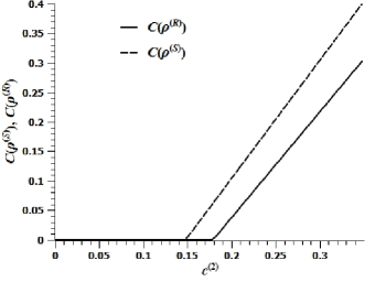
(a)

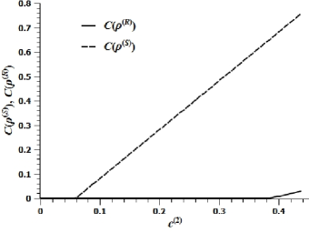
(b)

Figure 1: Case I: $\lambda^{(1)}\neq\lambda^{(2)}$, $c^{(1)}=0$, $c^{(2)}\geq 0$. Concurrences $C(\rho^{(S)})$ and $C(\rho^{(R)})$ as functions of $c^{(2)}$. (a) $N=6$, $c^{(2)}_{max}=0.3479$; (b) $N=42$, $c^{(2)}_{max}=0.4372$.

III.1.2 Case II: $\lambda^{1}\neq\lambda^{2}$, $c^{(1)}\geq 0$, $c^{(2)}=0$.

In this case, the behavior of concurrence significantly differs from Case I. First of all, the concurrence is nonlinear function of $c^{(1)}$, which is confirmed by Fig. 2. Next, the concurrence of the sender’s state $C(\rho^{(S)})=0$ if $c^{(1)}<c^{(1)}_{S;cr}$, while the concurrence of the receiver’s state $\rho^{(R)}$ is non-zero for all $c^{(1)}$. In addition, the concurrence in $\rho^{(S)}$ reaches larger values in the shorter chain ($N=6$, Fig.2a) than in the longer one ($N=42$, Fig.2b). Finally, $C(\rho^{(R)})>C(\rho^{(S)})$ over the allowed domain of $c^{(1)}$ except the case of the short chain with $c^{(1)}$ approaching $c^{(1)}_{max}$ as shown in Fig.2a.

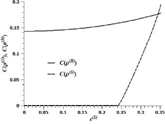
(a)

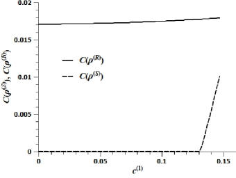
(b)

Figure 2: Case II: $\lambda^{(1)}\neq\lambda^{(2)}$, $c^{(1)}\geq 0$, $c^{(2)}=0$. Concurrences $C(\rho^{(S)})$ and $C(\rho^{(R)})$ as functions of $c^{(1)}$. (a) $N=6$, $c^{(1)}_{max}=0.3524$; (b) $N=42$, $c^{(1)}_{max}=0.1469$.

III.1.3 Case III: $\lambda^{1}\neq\lambda^{2}$, $c^{(1)}\geq 0$, $c^{(2)}\geq 0$.

This case combines the properties of the two previous ones, see Fig. 3, but there are certain differences. Fig.3a and Fig.3c show that the concurrence $C(\rho^{(S)})$ for $c^{(1)}=0$ approximately repeats the shapes shown in Fig.1, while $C(\rho^{(S)})$ for $c^{(2)}=0$ is less than the entanglement in Fig.2 and is zero for $N=42$. There is a critical line $(c^{(1)}_{S;cr},c^{(2)}_{S;cr})$ on the plane $(c^{(1)},c^{(2)})$ which bounds the region with zero concurrence (this boundary is not depicted explicitly in Fig.3a). The region of zero concurrence reduces with an increase in $N$.

The concurrence $C(\rho^{(R)})$ behaves in a different way, Fig.3b,d. At $c^{(2)}=0$, it approximately repeats the shape shown in Fig.2, while it is constant at $c^{(1)}=0$: $C(\rho^{(R)})|_{N=6}=0.1026$, $C(\rho^{(R)})|_{N=42}=0.0212$. Thus $\rho^{(R)}$ is nonzero for all positive $c^{(1)}$ and $c^{(2)}$ from the ellipse-like domain with the semi-axes $c^{(1)}_{max}$ and $c^{(2)}_{max}$. The Fig.3a and Fig.3c show that the concurrence in the sender $C(\rho^{(S)})$ reaches larger values for a long chain than for a short one, unlike the concurrence in the receiver. Comparing Fig.3a with Fig.3b (and Fig.3c with Fig.3d) we see that the maximum value of $C(\rho^{(S)})$ exceeds the maximum value of $C(\rho^{(R)})$ over $(c^{(1)},c^{(2)})$. But all the sender’s states with zero entanglement are mapped onto the receiver’s states with nonzero entanglement.

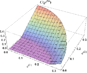
(a)

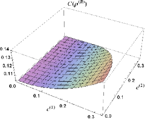
(b)

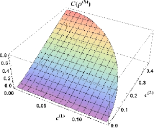
(c)

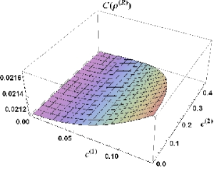
(d)

Figure 3: Case III: $\lambda^{(1)}\neq\lambda^{(2)}$, $c^{(1)}\geq 0$, $c^{(2)}\geq 0$. Concurrences $C(\rho^{(S)})$ and $C(\rho^{(R)})$ as functions of $c^{(1)}$ and $c^{(2)}$ over the quarter of the ellipse-like domain on the plane $(c^{(1)},c^{(2)})$. (a,b) $N=6$, the semi-axes $c^{(1)}_{max}=0.3216$ and $c^{(2)}_{max}=0.3369$; (a) $C(\rho^{(S)})$; (b) $C(\rho^{(R)})$. (c,d) $N=42$, the semi-axes $c^{(1)}_{max}=0.1322$ and $c^{(2)}_{max}=0.4526$; (c) $C(\rho^{(S)})$; (d) $C(\rho^{(R)})$.

III.1.4 Case IV: $\lambda^{1}=\lambda^{2}$, $c^{(1)}\geq 0$, $c^{(2)}\geq 0$.

Only the concurrence in $\rho^{(S)}$ is nonzero in this case. The shapes of graphs in Fig.4a,b are similar to that in Fig.3a,c, but the values of the concurrences are less in this case.

(a)

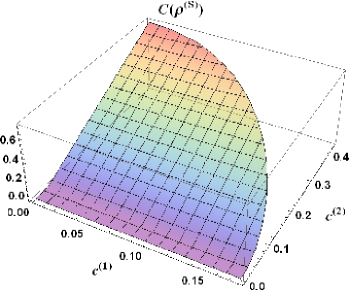
(b)

Figure 4: Case IV: $\lambda^{(1)}=\lambda^{(2)}$, $c^{(1)}\geq 0$, $c^{(2)}\geq 0$. Concurrence $C(\rho^{(S)})$ as a function of $c^{(1)}$ and $c^{(2)}$ over the quarter of the ellipse-like domain on the plane $(c^{(1)},c^{(2)})$. (a) $N=6$, semi-axes $c^{(1)}_{max}=0.3058$ and $c^{(2)}_{max}=0.3200$; (b) $N=42$, semi-axes $c^{(1)}_{max}=0.1789$ and $c^{(2)}_{max}=0.4283$.

IV Perturbations of block-scalable states and their influence on entanglement

IV.1 Perturbations of block-scalable states

The two-qubit receiver’s density matrix $\rho^{(R)}$ can be written in terms of the sender’s density matrix $\rho^{(S)}$ and the evolution operator $T$ as follows Z_JPA2012

$$\rho^{(R)}_{nm}(t)=\sum_{i,j=1}^{4}T_{nm,ij}(t)\rho^{(S)}_{ij}(0).$$ (22)

Since, on the other hand, $\rho^{(S)}$ and $\rho^{(R)}$ are representable as, respectively, sums (12) and (13), we conclude that in the unperturbed case, the evolution operator $T$ reduces to multiplication of $\rho^{(S;i)}$ and $\tilde{\rho}^{(S;0)}$ by the scale factors. In practice, we can not construct matrices $\rho^{(X;i)}$ in expansions (12) and (13) exactly, because of experimental and numerical errors. Therefore, the initial state can deviate from the required block-scalable state. Consequently, the quantum correlations in such state can differ from those calculated in Sec. III. This prompts us to compare the quantum correlations in block-scalable (block-scaled) states with those in states from their neighborhood. We introduce the perturbed MQ-coherence matrices $\rho^{(S;i)}(\varepsilon)$, $i=0,\pm 1,\pm 2$:

$$\tilde{\rho}^{(S;0)}(\varepsilon)=\tilde{\rho}^{(X;0)}+\sigma^{(S;0)}\varepsilon,$$ (23)

$$\rho^{(S;i)}(\varepsilon)+\rho^{(S;-i)}(\varepsilon)=(\rho^{(X;i)}+\rho^{(X;-i)}+(\sigma^{(S;i)}+\sigma^{(S;-i)})\varepsilon)c^{(i)},\;\;i=1,2.$$

Here, $\varepsilon$ is the perturbation amplitude, $\sigma^{(S;i)}$ is a perturbation of the $i$-order coherence matrix, $\sigma^{(S;0)}$ is a Hermitian matrix, ${\mbox{Tr}}\;\sigma^{(S;0)}=0$, and $(\sigma^{(S;i)})^{+}=\sigma^{(S;-i)}$. In addition, $\sigma^{(S)}$ must be such that the perturbed matrix $\rho^{(S)}$ remains a density matrix (Hermitian non-negative definite matrix with the unit trace) over the whole allowed domain in the plane $(c^{(1)},c^{(2)})$. Thus, the perturbed initial state reads

$$\rho^{(S)}(\varepsilon)=\rho^{(S)}(0)+\sigma^{(S)}\varepsilon,$$ (24)

where

$$\sigma^{(S)}=\sigma^{(S;0)}+(\sigma^{(S;1)}+\sigma^{(S;-1)})c^{(1)}+(\sigma^{(S;2)}+\sigma^{(S;-2)})c^{(2)}.$$ (25)

This results in the following perturbed receiver’s state:

$$\rho^{(R)}_{nm}(\varepsilon)=\sum_{i,j=1}^{4}T_{nm,ij}\rho^{(S)}_{ij}(0)+\sigma^{(R)}\varepsilon,$$ (26)

where

$$\sigma^{(R)}_{nm}=\sum_{i,j=1}^{4}T_{nm,ij}\sigma^{(S)}_{ij}\varepsilon.$$ (27)

We consider the random nondiagonal elements of $\sigma^{(S;k)}$, $k=0,1,2$, in the following form:

$$\sigma^{(S;k)}_{nm}=\sigma^{(k;1)}_{nm}e^{i\sigma^{(k;2)}_{nm}},\;\;k=0,1,2,\;\;n\neq m$$ (28)

$$0\leq\sigma^{(k;1)}_{nm}\leq 1,\;\;0\leq\sigma^{(k;2)}_{nm}\leq 2\pi.$$

To satisfy the normalization trace-condition for the diagonal elements we perturb them as follows:

$${\sigma^{(S;0)}_{nn}=\tilde{\sigma}_{nn}-\frac{1}{4}\sum_{i=1}^{4}\tilde{\sigma}_{ii},}\;\;-1\leq\tilde{\sigma}_{ii}\leq 1.$$ (29)

IV.2 Effect of block-scalable state perturbation on entanglement

Now we compare the concurrence of block-scalable and block-scaled states with the concurrence of the states from their neighborhood. With this aim, we consider the effect of perturbation described in Sec.IV.1 on the concurrence of both sender’s and receiver’s states averaging the calculated concurrence over 5000 (Secs.IV.2.1 and IV.2.2) or 1000 (Secs.IV.2.3 and IV.2.4) realizations of an arbitrary matrix $\sigma^{(S)}$. Hereafter $C$ denotes this mean concurrence. We consider one of the following sets of six perturbation amplitudes in the communication lines of $N=6$ and $N=42$ nodes:

$$\varepsilon=0.0125,\;0.025,\;0.05,\;0.1,\;0.2,\;1,\;\;{\mbox{in Secs. \ref{Section:a} and \ref{Section:b} }},$$ (30)

$$\varepsilon=0.0125,\;0.025,\;0.05,\;0.1,\;0.2,\;0.5,\;\;{\mbox{in Secs. \ref{Section:c} and \ref{Section:d} }}.$$

We include the large amplitude perturbations to explore the difference between the entanglements in the block-scalable (block-scaled) states and the entanglements in states which are far from them. Similar to Sec.III.1, we describe the entanglement in four cases indicated in the end of Sec.II.

IV.2.1 Case I: $\lambda^{1}\neq\lambda^{2}$, $c^{(1)}=0$, $c^{(2)}\geq 0$.

The perturbation of the sender’s initial state in this case reads

$$\sigma^{(S)}=\sigma^{(S;0)}+(\sigma^{(S;2)}+\sigma^{(S;-2)})c^{(2)}.$$ (31)

The mean concurrences in $\rho^{(S)}(0)$ and $\rho^{(R)}$ for set of $\varepsilon$ (30) are shown in Fig.5. This figure demonstrates that an increase in $\varepsilon$ leads to a decrease in $c^{(2)}_{S;cr}$ and $c^{(2)}_{R;cr}$. But the maximal value of concurrence $C_{max}(\rho^{(S)})$ (corresponding to $c^{(2)}_{max}$) increases with an increase in $\varepsilon$ till $\varepsilon\sim 0.2$ ($N=6$) or $\varepsilon\sim 0.05$ ($N=42$). But then it decreases with the further increase in $\varepsilon$, see Fig.5a,c. Similarly, $C_{max}(\rho^{(R)})$ in short chains increases with an increase in $\varepsilon$ till $\varepsilon\sim 0.1$. Then, $C_{max}(\rho^{(R)})$ decreases with the further increase in $\varepsilon$, see Fig.5b. But in the long chain ($N=42$), $C_{max}(\rho^{(R)})$ decreases with an increase in $\varepsilon$ till $\varepsilon\sim 1$, see Fig.5d.

(a)

(b)

(c)

(d)

Figure 5: Case I: $\lambda^{(1)}\neq\lambda^{(2)}$, $c^{(1)}=0$, $c^{(2)}\geq 0$. Concurrences $C(\rho^{(S)})$ and $C(\rho^{(R)})$ as functions of $c^{(2)}$ for different values of the perturbation amplitude $\varepsilon$ (30). (a,b) $N=6$, $c^{(2)}_{max}=0.3479$; (a) $C(\rho^{(S)})$, the lines corresponding to $\varepsilon=0$, 0.0125, $\dots$, 0.2 form a bunch where $\varepsilon$ increases in an upward direction; (b) $C(\rho^{(R)})$, the lines corresponding to $\varepsilon=0$, 0.0125, 0.025 form a bunch where $\varepsilon$ increases in an upward direction. (c,d) $N=42$, $c^{(2)}_{max}=0.4372$; (c) $C(\rho^{(S)})$, the lines corresponding to $\varepsilon=0$, 0.0125, 0.025, 0.05, 0.1 form a bunch; the line $\varepsilon=0.1$ crosses all other lines in this bunch and becomes the lower one near $c^{(2)}_{max}$; other lines in this bunch do not cross each other, $\varepsilon$ of these lines increases in upward direction; inset shows the behavior of the concurrences for small $c^{(2)}$; (d) $C(\rho^{(R)})$.

IV.2.2 Case II: $\lambda^{1}\neq\lambda^{2}$, $c^{(1)}\geq 0$, $c^{(2)}=0$.

The perturbation of the sender’s initial state in this case reads

$$\sigma^{(S)}=\sigma^{(S;0)}+(\sigma^{(S;1)}+\sigma^{(S;-1)})c^{(1)}.$$ (32)

The mean concurrences for set of $\varepsilon$ (30) are shown in Fig.6. This figure demonstrates that an increase in $\varepsilon$ leads to a decrease in $c^{(1)}_{S;cr}$. Also the maximal concurrence $C_{max}(\rho^{(S)})$ (corresponding to $c^{(1)}_{max}$) decreases with an increase in $\varepsilon$ in a short chain, see Fig. 6a. In the long chain ($N=42$), it decreases till $\varepsilon\sim 0.2$ and then it increases with an increase in $\varepsilon$, see Fig.6c. Behavior of $C(\rho^{(R)})$ is different, see Fig.6b and Fig.6d. First of all, it is positive for all $c^{(1)}$. $C_{max}(\rho^{(R)})$ decreases with $\varepsilon$ till $\varepsilon\sim 0.0125$ in both short ($N=6$) and long ($N=42$) chains, and then it increases with the further increase in $\varepsilon$. For the long chain, the large deviation from the block-scalable state ($\varepsilon=1$) significantly increases the concurrence in the sender and receiver for all $c^{(1)}$, as shown in Fig.6c,d. For the short chain, this holds only for $C(\rho^{(R)})$, Fig.6b

(a)

(b)

(c)

(d)

Figure 6: Case II: $\lambda^{(1)}\neq\lambda^{(2)}$, $c^{(1)}\geq 0$, $c^{(2)}=0$. Concurrences $C(\rho^{(S)})$ and $C(\rho^{(R)})$ as functions of $c^{(1)}$ for different values of the perturbation amplitude $\varepsilon$ (30). (a,b) $N=6$, $c^{(1)}_{max}=0.3524$; (a) $C(\rho^{(S)})$; (b) $C(\rho^{(R)})$, the lines $\varepsilon=0$ and $0.05$ cross each other. (c,d) $N=42$, $c^{(1)}_{max}=0.1469$; (c) $C(\rho^{(S)})$, the lines corresponding to $\varepsilon=0.1$ and 0.2 are indistinguishable from the axis of abscissas; at $c^{(2)}_{max}$, $C_{max}(\rho^{(S)})$ decreases with an increase in $\varepsilon$ till $\varepsilon\sim 0.2$ and increases after that; (d) $C(\rho^{(R)})$, the order of $\varepsilon$ is shown in figure.

IV.2.3 Case III: $\lambda^{1}\neq\lambda^{2}$, $c^{(1)}\geq 0$, $c^{(2)}\geq 0$.

The perturbation of the sender’s initial state in this case reads

$$\sigma^{(S)}=\sigma^{(S;0)}+(\sigma^{(S;1)}+\sigma^{(S;-1)})c^{(1)}+(\sigma^{(S;2)}+\sigma^{(S;-2)})c^{(2)}.$$ (33)

We characterize the effect of perturbations by the extrema $C_{max}=\displaystyle\min_{c^{(1)},c^{(2)}}C$ and $C_{min}=\displaystyle\max_{c^{(1)},c^{(2)}}C$ as functions of $\varepsilon$ in Fig.7. The numerical study shows that the functions $C(\rho^{(S)})$ and $C(\rho^{(R)})$ take their maximal and minimal values at the same points on the plane $(c^{(1)},c^{(2)})$ for all perturbations:

$$C_{min}(\rho^{(S)}(0))=\min_{c^{(1)},c^{(2)}}C(\rho^{(S)}(0))=C(\rho^{(S)}(0))|_{{c^{(1)}=0}\atop{c^{(2)}=0}},$$ (34)

$$C_{max}(\rho^{(S)}(0))=\max_{c^{(1)},c^{(2)}}C(\rho^{(S)}(0))=C(\rho^{(S)}(0))|_{{c^{(1)}=0}\atop{c^{(2)}=c^{(2)}_{max}}},$$

$$C_{min}(\rho^{(R)})=\min_{c^{(1)},c^{(2)}}C(\rho^{(R)})=C(\rho^{(R)})|_{{c^{(1)}=0}\atop{c^{(2)}=0}},$$

$$C_{max}(\rho^{(R)})=\max_{c^{(1)},c^{(2)}}C(\rho^{(R)})=C(\rho^{(R)})|_{{c^{(1)}=c^{(1)}_{max}}\atop{c^{(2)}=0}}.$$

Figs.7a and 7c demonstrate that the minimal value of $C(\rho^{(S)})$ equals zero for all $\varepsilon$, while $C_{max}(\rho^{(S)})$ in the short chain ($N=6$) has a weakly formed maximum at $\varepsilon\sim 0.025$, and then it decreases with an increase in $\varepsilon$. The behavior of $C(\rho^{(R)})$ is different, Fig.7b,d. Its minimal value is never zero and both minimal and maximal values generally increase with an increase in $\varepsilon$ for large $\varepsilon$. In the short chain of $N=6$ nodes, both $C_{min}(\rho^{(R)})$ and $C_{max}(\rho^{(R)})$ have a minimum at $\varepsilon\sim 0.05$. We also notice that the minimal and maximal values of $C(\rho^{(R)})$ approach each other in long chains, as shown in Fig.7d. In other words, the concurrence tends to the constant value in this case.

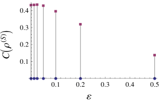
(a)

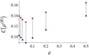
(b)

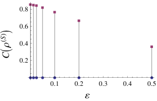
(c)

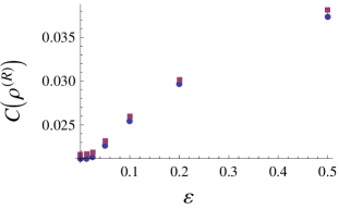
(d)

Figure 7: Case III: $\lambda^{(1)}\neq\lambda^{(2)}$, $c^{(1)}\geq 0$, $c^{(2)}\geq 0$. Maximal (squares) and minimal (circles) values of the concurrences $C(\rho^{(S)})$ and $C(\rho^{(R)})$ (34) as functions of $\varepsilon$. (a) $N=6$, $C(\rho^{(S)})$; (b) $N=6$, $C(\rho^{(R)})$; (c) $N=42$, $C(\rho^{(S)})$; (d) $N=42$, $C(\rho^{(R)})$.

IV.2.4 Case IV: $\lambda^{1}=\lambda^{2}$, $c^{(1)}\geq 0$, $c^{(2)}\geq 0$.

The perturbation of the sender’s initial state in this case is as in (33). The extrema $\displaystyle C_{min}(\rho^{(S)})$ and $\displaystyle C_{max}(\rho^{(S)})$ (34) as functions of $\varepsilon$ are shown in Fig.8. We see that the behavior of the maximal and minimal values of $C(\rho^{(S)})$ in Fig.8a,c is very similar to that in Case III, Sec.IV.2.3. The only difference is the presence of a well formed maximum at $\varepsilon\sim 0.05$ in the short chain of $N=6$ spins and a weakly formed maximum at $\varepsilon\sim 0.0125$ in the long chain. On the contrary, $C(\rho^{(R)})$ is nonzero only for large $\varepsilon$ ($\varepsilon\sim 0.5$). In this case, again the minimal and maximal values of $C(\rho^{(R)})$ approach each other in the long chain with $N=42$, i.e, the concurrence is nearly independent on $c^{(1)}$ and $c^{(2)}$ for all perturbation amplitudes $\varepsilon$, see Fig.8d.

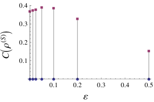
(a)

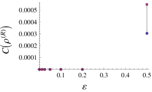
(b)

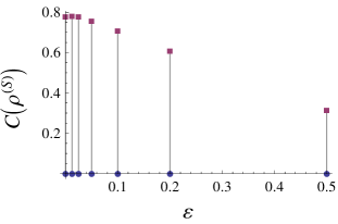
(c)

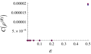
(d)

Figure 8: Case IV: $\lambda^{(1)}=\lambda^{(2)}$, $c^{(1)}\geq 0$, $c^{(2)}\geq 0$. Maximal (squares) and minimal (circles) values of the concurrences $C(\rho^{(S)})$ and $C(\rho^{(R)})$ as functions of $\varepsilon$. (a) $N=6$, $C(\rho^{(S)})$; (b) $N=6$, $C(\rho^{(R)})$; (c) $N=42$, $C(\rho^{(S)})$; (d) $N=42$, $C(\rho^{(R)})$.

From the analysis of Cases I – IV in Secs.IV.2.1-IV.2.4 we conclude that in the framework of our consideration, the maximal value of concurrence in the block-scalable sender’s initial states, $\displaystyle C_{max}(\rho^{(S)}(0))$, reaches larger values than that in the states from the remote neighborhood ($\varepsilon=1$ in Cases I, II and $\varepsilon=0.5$ in Cases III, IV ), except in the case $c^{(2)}=0$, $N=42$ (long chain), Fig.6c. However, the corresponding concurrence $\displaystyle C_{max}(\rho^{(R)})$ in the receiver’s block-scaled states is smaller than that in the states from the remote neighbourhood (except the Case I, Fig.5b,d). This is the price to pay for the simple and well-described deformation of the transferred quantum state. Regarding the uniform scaling in Case IV, Sec.IV.2.4 ($\lambda^{(1)}=\lambda^{(2)}$), the concurrence in the block-scaled states does not appear at all in the settings of our numerical simulations except the case of large-amplitude perturbations ($\varepsilon=0.5$), Fig.8b,d.

V Conclusions

The block-scaled state transfer is a method for remote state creation such that the state created at the receiver is similar to the initial sender’s state with a minimal, well-described deformation. This deformation appears as the scale factors in front of certain blocks (MQ-coherence matrices) of the initial sender’s state except the only diagonal element which must satisfy the trace condition. In this case the initial sender’s state is referred to as the block-scalable state.

Since the map (block-scalable state) $\to$ (block-scaled state) can be simply described, it is interesting to find out features of quantum correlations in such states. These correlations are studied in our paper in terms of entanglement (concurrence) in spin chains with 2-qubit sender and receiver. We find out the dependence of the concurrence on the parameters $c^{(1)}$ and $c^{(2)}$ transferred by the $\pm 1$- and $\pm 2$-order coherence matrices. There are certain differences in concurrences for the four cases outlined in the end of Sec.II. Thus, in Case I, the concurrence appears only for large $c^{(2)}$ in both $\rho^{(S)}$ and $\rho^{(R)}$. In Case II, the concurrence in $\rho^{(S)}$ appears for large $c^{(1)}$, while the concurrence in $\rho^{(R)}$ appears for all $c^{(1)}$. Case III combines properties of Cases I and II, but $C(\rho^{(R)})$ is nonzero for all values of $c^{(1)}$ and $c^{(2)}$ from their domain. Case IV differs from others by having zero concurrence in the receiver’s state. Generally, the concurrence in the block-scalable states reaches significantly larger values than the concurrence in the block scaled states.

Next, we estimate the difference between the entanglement in the block-scalable (block-scaled) states and in the states from their close and remote neighborhoods. To this end, we study the effect of perturbations of the initial block-scalable states on the entanglement and show that this effect depends on which of the higher order coherence matrices are involved in the process. Thus, if only the zeroth- and $\pm 2$-order coherences are transferred (Case I), then, for the small perturbations, entanglement appears only for large enough $c^{(2)}$ in both $\rho^{(S)}$ and $\rho^{(R)}$. But eventually for $\varepsilon\sim 1$, entanglement appears for all $c^{(2)}$ and its maximal value is significantly smaller then that for the unperturbed case. If only zeroth- and $\pm 1$-order coherences are used (Case II), then the entanglement $C(\rho^{(S)})$ appears for large $c^{(1)}$ if $\varepsilon\ll 1$. But, for $\varepsilon\sim 1$, this entanglement appears for all $c^{(1)}$ and, in long chains, it becomes significantly larger than the entanglement in the unperturbed case. The entanglement of the receiver state $C(\rho^{(R)})$ exists for all $c^{(1)}$ and it generally increases (except the very small perturbations amplitudes $\varepsilon$) with an increase in $\varepsilon$. In both these cases, the critical values $c^{(1)}_{S;cr}$, $c^{(1)}_{R;cr}$ and $c^{(2)}_{S;cr}$ decrease with an increase in $\varepsilon$. If all three coherence matrices are involved (Case III), then the maximal value of entanglement as a function of $c^{(1)}$ and $c^{(2)}$ generally decreases with an increase in $\varepsilon$ in the sender, while it generally increases in the receiver. If $\lambda^{(1)}=\lambda^{(2)}$ (Case IV), then the entanglement in the sender behaves similar to the previous case, and the entanglement in the receiver $C(\rho^{(R)})$ becomes non-zero only for large-amplitude perturbations. In Cases II-IV applied to a long chain ($N=42$), the entanglement in the receiver $C(\rho^{(R)})$ only slightly depends on the parameters $c^{(1)}$ and $c^{(2)}$.

Thus, the block-scaled state transfer is a variant of a state evolution with a simple and well-described state deformation. Usually, the entanglement of the receiver’s block-scaled state is less than the entanglement in the corresponding sender’s block-scalable state. The entanglement in the block-scaled state can even vanish. Large perturbation of a block-scalable state leads to a decrease in concurrence $C(\rho^{(S)})$ and to an increase in concurrence $C(\rho^{(R)})$. In addition, the evolution generally reduces the dependence of concurrence on the parameters $c^{(1)}$ and $c^{(2)}$ in long chains, which is referred to both unperturbed and perturbed cases considered in this paper.

This work was performed in accordance with the state task, state registration No. 0089-2019-0002, and was partially supported by the program of the Presidium of RAS No. 5 ”Photonic technologies in probing inhomogeneous media and biological objects”.

VI Appendix: Explicit form of block-scalable ($\rho^{(S)}(0)$) and block-scaled ($\rho^{(S)}(t)$) density matrices

We present the density matrices used in the numerical calculations of Sec.III.1. More details can be found in Ref.BFZ_Arch2018 where these matrices are constructed as a result of the optimization procedure. In formulas (44)-(79) below we use the following notation:

$$\Lambda^{(0)}=\left\{\begin{array}[]{cc}1,&\rho^{(B)}=\rho^{(S)}\cr\lambda^{(0)},&\rho^{(B)}=\rho^{(R)}\end{array}\right.,\;\;{\Lambda^{(n)}=\left\{\begin{array}[]{cc}c^{(n)},&\rho^{(B)}=\rho^{(S)}\cr c^{(n)}\lambda^{(n)},&\rho^{(B)}=\rho^{(R)}\end{array}\right.,\;\;n=1,2.}$$ (39)

1. $\lambda^{1}\neq\lambda^{2}$, $c^{(1)}=0$, $c^{(2)}\geq 0$, $\lambda^{(0)}(6)=1.08371$, $\lambda^{(2)}(6)=0.89602$, $t(6)=8.51533$, $b(6)=b(42)=10$, $\lambda^{(0)}(42)=1.69754$, $\lambda^{(2)}(42)=0.26204$, $t(42)=47.97194$,

   $$\rho^{(B)}(6)=\left(\begin{array}[]{cccc}0.40596\Lambda^{(0)}&0&0&\Lambda^{(2)}\cr 0&0.15131\Lambda^{(0)}&0.00010i\Lambda^{(0)}&0\cr 0&-0.00010i\Lambda^{(0)}&0.14467\Lambda^{(0)}&0\cr\Lambda^{(2)}&0&0&1-0.70194\Lambda^{(0)}\end{array}\right).$$ (44)

   $$\rho^{(B)}(42)=\left(\begin{array}[]{cccc}0.44635\Lambda^{(0)}&0&0&\Lambda^{(2)}\cr 0&0.08266\Lambda^{(0)}&0.01664i\Lambda^{(0)}&0\cr 0&-0.01664i\Lambda^{(0)}&0.04275\Lambda^{(0)}&0\cr\Lambda^{(2)}&0&0&1-0.57176\Lambda^{(0)}\end{array}\right).$$ (49)

2. $\lambda^{1}\neq\lambda^{2}$, $c^{(1)}\geq 0$, $c^{(2)}=0$, $\lambda^{(0)}(6)=1.22015$, $\lambda^{(1)}(6)=0.81452$, $t(6)=5.03255$, $b(6)=10$, $\lambda^{(0)}(42)=1.36938$, $\lambda^{(1)}(42)=0.31866$, $t(42)=41.32805$, $b(42)=7.02476$,

   $$\rho^{(B)}(6)=\left(\begin{array}[]{cccc}0.59440\Lambda^{(0)}&0.77790\Lambda^{(1)}&-0.62839i\Lambda^{(1)}&0\cr 0.77790\Lambda^{(1)}&0.12890\Lambda^{(0)}&-0.10707i\Lambda^{(0)}&-0.00003i\Lambda^{(1)}\cr 0.62839i\Lambda^{(1)}&0.10707i\Lambda^{(0)}&0.09232\Lambda^{(0)}&-0.00004\Lambda^{(1)}\cr 0&0.00003i\Lambda^{(1)}&-0.00004\Lambda^{(1)}&1-0.81562\Lambda^{(0)}\end{array}\right).$$ (54)

   $$\rho^{(B)}(42)=\left(\begin{array}[]{cccc}0.68654\Lambda^{(0)}&0.92494\Lambda^{(1)}&-0.38010i\Lambda^{(1)}&0\cr 0.92494\Lambda^{(1)}&0.03320\Lambda^{(0)}&-0.01710i\Lambda^{(0)}&-0.00034i\Lambda^{(1)}\cr 0.38010i\Lambda^{(1)}&0.01710i\Lambda^{(0)}&0.01035\Lambda^{(0)}&-0.00082\Lambda^{(1)}\cr 0&0.00034i\Lambda^{(1)}&-0.00082\Lambda^{(1)}&1-0.73008\Lambda^{(0)}\end{array}\right).$$ (59)

3. $\lambda^{1}\neq\lambda^{2}$, $c^{(1)}\geq 0$, $c^{(2)}\geq 0$, $\lambda^{(0)}(6)=1.26340$, $\lambda^{(1)}(6)=0.76126$, $\lambda^{(2)}(6)=0.22885$, $t(6)=5.37677$, $b(6)=5.37902$, $\lambda^{(0)}(42)=1.53227$, $\lambda^{(1)}(42)=0.29521$, $\lambda^{(2)}(42)=0.03935$, $t(42)=41.94097$, $b(42)=6.87959$,

   $$\rho^{(B)}(6)=\left(\begin{array}[]{cccc}0.51945\Lambda^{(0)}&0.88361\Lambda^{(1)}&-0.46820i\Lambda^{(1)}&\Lambda^{(2)}\cr 0.88361\Lambda^{(1)}&0.18237\Lambda^{(0)}&-0.11342i\Lambda^{(0)}&-0.00216i\Lambda^{(1)}\cr 0.46820i\Lambda^{(1)}&0.11342i\Lambda^{(0)}&0.07949\Lambda^{(0)}&-0.00408\Lambda^{(1)}\cr\Lambda^{(2)}&0.00216i\Lambda^{(1)}&-0.00408\Lambda^{(1)}&1-0.78130\Lambda^{(0)}\end{array}\right).$$ (64)

   $$\rho^{(B)}(42)=\left(\begin{array}[]{cccc}0.58895\Lambda^{(0)}&0.96932\Lambda^{(1)}&-0.24580i\Lambda^{(1)}&\Lambda^{(2)}\cr 0.96932\Lambda^{(1)}&0.05117\Lambda^{(0)}&-0.02255i\Lambda^{(0)}&-0.00025i\Lambda^{(1)}\cr 0.24580i\Lambda^{(1)}&0.02255i\Lambda^{(0)}&0.01209\Lambda^{(0)}&-0.00010\Lambda^{(1)}\cr\Lambda^{(2)}&0.00025i\Lambda^{(1)}&-0.00010\Lambda^{(1)}&1-0.65221\Lambda^{(0)}\end{array}\right).$$ (69)

4. $\lambda^{1}=\lambda^{2}$, $c^{(1)}\geq 0$, $c^{(2)}\geq 0$, $\lambda^{(0)}(6)=1.2022$, $\lambda^{(1)}(6)=\lambda^{(2)}(6)=0.2956$, $t(6)=5.6651$, $b(6)=2.3462$, $\lambda^{(0)}(42)=1.42581$, $\lambda^{(1)}(42)=\lambda^{(2)}(42)=0.04943$, $t(42)=42.3077$, $b(42)=3.8922$,

   $$\rho^{(B)}(6)=\left(\begin{array}[]{cccc}0.49962\Lambda^{(0)}&0.98333\Lambda^{(1)}&-0.15484i\Lambda^{(1)}&\Lambda^{(2)}\cr 0.98333\Lambda^{(1)}&0.20645\Lambda^{(0)}&-0.07298i\Lambda^{(0)}&-0.01482i\Lambda^{(1)}\cr 0.15484i\Lambda^{(1)}&0.07298i\Lambda^{(0)}&0.08884\Lambda^{(0)}&-0.09414\Lambda^{(1)}\cr\Lambda^{(2)}&0.01482i\Lambda^{(1)}&-0.09414\Lambda^{(1)}&1-0.79491\Lambda^{(0)}\end{array}\right).$$ (74)

   $$\rho^{(B)}(42)=\left(\begin{array}[]{cccc}0.61003\Lambda^{(0)}&0.99758\Lambda^{(1)}&-0.06640i\Lambda^{(1)}&\Lambda^{(2)}\cr 0.99758\Lambda^{(1)}&0.06660\Lambda^{(0)}&-0.02143i\Lambda^{(0)}&-0.00135i\Lambda^{(1)}\cr 0.06640i\Lambda^{(1)}&0.02143i\Lambda^{(0)}&0.02265\Lambda^{(0)}&-0.02035\Lambda^{(1)}\cr\Lambda^{(2)}&0.00135i\Lambda^{(1)}&-0.02035\Lambda^{(1)}&1-0.69928\Lambda^{(0)}\end{array}\right).$$ (79)

References

- (1) S. Bose, Phys. Rev. Lett. 91, 207901 (2003)
- (2) M.Christandl, N.Datta, A.Ekert, and A.J.Landahl, Phys.Rev.Lett. 92, 187902 (2004)
- (3) C.Albanese, M.Christandl, N.Datta, and A.Ekert, Phys.Rev.Lett. 93, 230502 (2004)
- (4) P.Karbach and J.Stolze, Phys.Rev.A 72, 030301(R) (2005)
- (5) G.Gualdi, V.Kostak, I.Marzoli, and P.Tombesi, Phys.Rev. A 78, 022325 (2008)
- (6) A.Wójcik, T.Luczak, P.Kurzyński, A.Grudka, T.Gdala, and M.Bednarska Phys. Rev. A 72, 034303 (2005)
- (7) N.A.Peters, J.T.Barreiro, M.E.Goggin, T.-C.Wei, and P.G.Kwiat, Phys.Rev.Lett. 94, 150502 (2005)
- (8) N.A.Peters, J.T.Barreiro, M.E.Goggin, T.-C.Wei, and P.G.Kwiat in Quantum Communications and Quantum Imaging III, ed. R.E.Meyers, Ya.Shih, Proc. of SPIE 5893 (SPIE, Bellingham, WA, 2005)
- (9) G.Y. Xiang, J.Li, B.Yu, and G.C.Guo, Phys. Rev. A 72, 012315 (2005)
- (10) G. A. Bochkin and A. I. Zenchuk, Phys.Rev.A 91, 062326(11) (2015)
- (11) J.Wei,L. Shi, Yu Zhu, Ya. Xue, Zh. Xu, J. Jiang, Quant.Inf.Proc. 17, 70 (2018)
- (12) J. Wei, L. Shi, J. Luo, Y.Zhu, Q. Kang, L.Yu, H. Wu, J. Jiang, B. Zhao, Quant.Inf.Proc. 17, 141 (2018)
- (13) J.Wei, L. Shi, L. Ma, Ya. Xue, X. Zhuang, Q. Kang, X. Li, Quant. Inf. Proc. 16, 260 (2017)
- (14) F.Shahandeh, A.P.Lund, T.C.Ralph, and M.R.Vanner, New J. Phys. 18, 103020 (2016)
- (15) N.M.VanMeter, P. Lougovski, D.B.Uskov, K.Kieling, J. Eisert, and J.P.Dowling, Phys. Rev. A 76, 063808 (2007)
- (16) C.H.Bennett, G.Brassard, C.Crépeau, R.Jozsa, A.Peres, and W.K.Wootters, Phys. Rev. Lett. 70, 1895 (1993)
- (17) D.Bouwmeester, J.-W. Pan, K.Mattle, M.Eibl, H.Weinfurter, and A. Zeilinger, Nature 390, 575 (1997)
- (18) D. Boschi, S. Branca, F. De Martini, L. Hardy, and S. Popescu, Phys. Rev. Lett. 80, 1121 (1998)
- (19) G.A.Bochkin, E.B.Fel’dman, A.I.Zenchuk, Quant.Inf.Proc. 17, 218 (2018)
- (20) E.B.Fel’dman, A.I.Zenchuk, JETP 125, 1042 (2017)
- (21) S.Hill and W.K.Wootters, Phys. Rev. Lett. 78, 5022 (1997)
- (22) W.K. Wootters, Phys. Rev. Lett. 80, 2245 (1998)
- (23) A.I.Zenchuk, J. Phys. A: Math. Theor. 45, 115306 (2012)