Logarithmic-layer turbulence: a view from the wall

Abstract

The observability of the flow away from the wall in turbulent channels is studied using noiseless, although potentially incomplete, wall measurements. Reconstructions of the velocities are generated using linear stochastic estimation. All the velocities are well reconstructed in the buffer layer, but only relatively large ‘wall-attached’ eddies are observable farther from the wall. In particular, large-scale structures that account for approximately 50% of the total kinetic energy and of the tangential Reynolds stress are accurately captured up to $y/h\lesssim 0.2$. It is argued that this should allow the use of wall sensors for the detection (and potential control) of the large eddies populating the logarithmic region, and that it suggests a natural quantitative definition for ‘wall-attached’ eddies.

I Introduction

This paper deals with the possibility of observing the flow far from the wall in a turbulent channel, using only measurements at the wall. There are at least two reasons why this may be desirable. The first one is purely scientific, because the relation between the near-wall and outer flows has been one of the most controversial questions in wall-bounded turbulence, and it stands to reason that influence and observability are related. If A does not influence B, it is unlikely that the former can be reconstructed from observations of the latter, and, conversely, if A can be reconstructed from B, it is unlikely that the two are completely unrelated. Note that the inverse is not true, especially if, as in this paper, we restrict ourselves to linear reconstructions. If A cannot be reconstructed from B, it cannot be concluded that the two are independent. In addition, reconstruction by itself does not give information on the direction of causality, if any. That B reconstructs A does not imply that B causes A, or the other way around. We focus on variables that can be reconstructed from wall measurements, and, in that regard, we will be able to propose criteria for which variables are ‘attached’ at what scales, in the sense that their influence extends to the wall, although these criteria might not coincide with Townsend’s dynamical definition of attached structures [1]. On the other hand, although it is probable that variables that cannot be reconstructed from the wall are ‘detached’, in the sense of having little or no influence over it, it follows from the previous discussion that this cannot be guaranteed.

A second reason for our interest in reconstruction is the possibility of active control of wall turbulence. This is a classic goal of turbulence research, whether to decrease or increase wall friction, reduce noise or other applications. Transportation of fluids through pipes, such as oil, gas or water, would benefit from drag reduction, and so would vehicles moving in fluids. In other engineering applications, such as combustion or heat transfer, or even aerodynamics, it may be desirable to increase the turbulent intensities close to walls to promote mixing or to delay separation. There is a well-developed theory for the optimal control of linear systems, and, although turbulence is nonlinear, there is extensive evidence that a substantial fraction of the dynamics of shear-driven flows can be linearised [2]. This has led to heuristic and theoretical active-control schemes that manipulate friction in turbulent channels at moderate Reynolds numbers, at least in simulations [3, 4], but they are not free from problems and ambiguities.

The first problem has to do with the scales involved. Most of the dissipation in wall-bounded flows is contained within or below the logarithmic layer (see figure 1a), suggesting that effective control should act near the wall. As a consequence, most schemes have targeted the buffer-layer, which contains the strongest turbulent fluctuations, but technological considerations suggest that practical applications should rather centre on the logarithmic-layer eddies. Thus, for a flow of thickness $h$ and Reynolds number $Re_{\tau}=u_{\tau}h/\nu$, where the ‘+’ superscript denotes wall units based on the friction velocity $u_{\tau}$ and on the kinematic viscosity $\nu$, the sizes and passing times of the structures in the buffer layer decrease proportionally to $Re_{\tau}$ when expressed in outer units. On the contrary, when the distance, $y$, from the wall is a fixed fraction of $h$, sizes and times scale in outer units, or at most depend logarithmically on the Reynolds number. For example, in a water pipe with $h\approx 1$ m and bulk velocity $U\approx 1$ m/s $(Re_{\tau}\approx 10^{5})$, the wall-normal velocity eddies in the buffer-layer have length and time scales of $\Delta x\approx 1$ mm $(\Delta x^{+}=100)$ and $\Delta t\approx 0.1$ ms, but those at a distance from the wall $y/h\approx 0.1$ are $\Delta x\approx 20$ cm and $\Delta t\approx 0.2$ s, where $\Delta x$ is the streamwise length. Similar differences apply to the flow over aeroplane wings.

However, moving away from the wall is not without cost. Figure 1(a) presents the fraction of the total dissipation below a given distance from the wall as a function of the Reynolds number [5]. An ‘ideal’ control strategy would probably result on the complete elimination of the turbulent energy dissipation over some part of the channel. Below $y^{+}=20$, most of the dissipation is due to the mean shear, and is independent of fluctuations. Centring on the remaining dissipation, in the example above, the velocity fluctuations in the logarithmic region, defined as $80\nu/u_{\tau}\leq y\leq 0.2h$, are responsible for about 40% of the energy loss, but the scales in its lower limit are those discussed above as being too small. If we want to restrict ourselves to fixed fractions of the flow thickness, to avoid wall scaling, the maximum fraction of the drag that could potentially be saved by completely removing all the dissipation between $y/h=0.01$ and 0.2 would be approximately 25% (at $Re_{\tau}\approx 10^{5}$). Decreasing the lower limit of wall distances increases the potential gain, but at the cost of having to deal with smaller length and time scales. Raising the upper limit is less effective. These estimations are only upper bounds, because turbulent dissipation can probably not be completely damped, but they show that the logarithmic layer is a ‘preferred region’ in which some control authority still remains, while the size of the eddies stays bounded from below as the Reynolds number increases.

A second problem is that most active-control schemes assume knowledge of the flow at wall distances of the order of the size of the structures to be controlled. Typically, the assumption is that the flow is fully known, as in direct numerical simulation (DNS), or at least that a two-dimensional section of some variables is available, as in particle-image velocimetry. Unfortunately, most practical observations are limited to the wall, where the only accessible variables are the pressure and the two shears. This problem is especially acute when we are interested in the logarithmic layer, which is separated from the wall by the very active buffer layer. Figure 1(b) shows spectra of the three observable variables at the wall. All of them are dominated by a core whose position scales in wall units, but they also include a larger-scale component, which is long for the two shears and wide for the pressure, with wavelengths that scale proportionally to $h$, and which are associated with eddies farther from the wall [6].

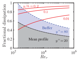
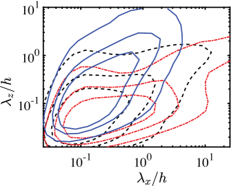
(a)  (b)

Figure 1: (a) Fraction of the total energy dissipation below a given distance from the wall, as a function of the Reynolds number. The dashed lines are scaled in wall units, and the labels refer to the predominant contributor to the dissipation in each region. The solid lines are three distances from the wall, scaled in outer units [adapted from 5]. (b) Premultiplied spectra of [6] at $y^{+}=5$;                   , streamwise stress;            , spanwise stress;   , pressure. The contours of each spectrum contain 50%, 70% and 90% of its spectral mass. $\lambda_{x}$ and $\lambda_{z}$ are respectively the streamwise and spanwise wavelengths.

This paper focuses on the properties of the estimations of logarithmic-layer turbulence using noiseless, although potentially incomplete, wall measurements from DNS. The widespread availability of data in the last years has allowed various research groups to test the performance of similar methods with considerable success [7, 8, 9, 10, 11]. These works differ from ours in that most of them focus on the use of physically motivated linear models [9, 10] to relate velocity measurements at one $y$ to predict the same velocity component at another wall-normal distance. Others [12, 11], also explore the performance of nonlinear models, with modest gains over their proposed linear method. In contrast, our methodology is linear regression, which has been successfully used for conditional flow reconstruction away from walls [13], or to synthesise buffer-layer velocities from experimental measurements farther away [7]. This ‘linear stochastic estimation’ (LSE), although apparently naive, is statistically optimal for linear systems, and we will show that it is adequate to reconstruct the Reynolds-stress structures in the logarithmic layer, using only variables that can be measured at the wall. A closely related investigation is [14], which analyses the correlation between wall pressure at the wall-normal velocity farther into the flow, but, to our knowledge the present paper is the first to one to use the full set of wall observables to reconstruct the full internal flow field, including the relative importance of the different observables on the three velocity components, and the identification of the accessible scales. Finally, it should be noted that, although not specifically addressed in the present work, similar methods should apply to transitional flows, where scales are typically larger, the role of linearity is more pronounced, and are thus more amenable to active control.

The remainder of this paper is organised as follows. The numerical datasets and the details of the reconstruction algorithm are presented in §II and §III, respectively. Section IV discusses the properties of the reconstruction, and §V concludes. Some preliminary work on the reconstruction of vorticity using similar techniques was performed at the 2018 CTR Stanford Summer Program [15], and an early partial version of the present manuscript is [16].

II Numerical experiments

We consider incompressible flow in channels whose half-height is $h$. The streamwise, wall-normal and spanwise directions are $x,y,z,$ respectively, and $u,v,w,p$ are the fluctuations of the corresponding velocity components and of the kinematic pressure. Capitals are used for averaged quantities, and primes for standard deviations. The computational domain is periodic in both wall-parallel directions, with periods $L_{x}$ and $L_{z}$. The spatial discretisation is Fourier spectral in those directions, dealiased using the $2/3$ rule, and compact finite differences or Chebyshev expansions in the wall-normal direction, depending on the Reynolds number. Table 1 collects basic information on the simulations, and refers to the original publications for further details.

Table 1: Parameters of the simulations. $L_{x,z}$ are the streamwise and spanwise period of the numerical box, and $N_{x,y,z}$ are the number of collocation points of the stored grid in each direction. $\Delta_{x}^{+},\Delta_{z}^{+}$ are the stream and spanwise grid resolutions of the DNS. $\Delta_{y_{\max(\min)}}^{+}$ is te maximum (minimum) resolution across the wall-normal direction. $Tu_{\tau}/h$ is the time spanned by the aproximatelly equispaced snapshots in eddy turnovers. $D_{y}$ represents the discretisation used for the wall-normal direction: ‘CH’ refers to Chebyshev polynomials and ‘FD’ to compact finite differences. $N_{f}$ is the number of fields used to compute statistics.

Name	$\mbox{{Re}}_{\tau}$	$(L_{x},L_{z})/h$	$N_{x}$	$N_{y}$	$N_{z}$	$\Delta x^{+}$	$\Delta z^{+}$	$\Delta y^{+}_{\max{}(\min{\!})}$	$Tu_{\tau}/h$	$D_{y}$	$N_{f}$	Reference
S1000	932	$(2\pi,\pi)$	$512$	$385$	$512$	12	6	7.7(0.03)	18	CH	$1800$	[17]
S2000	2003	$(2\pi,\pi)$	$1024$	$633$	$1024$	12	6	8.9(0.3)	11	FD	$800$	[17]
F2000	2003	$(8\pi,3\pi)$	$512$	$512$	$512$	24	9	10.6(1.7)	14	FD	$1200$	[18]
F5300	5300	$(8\pi,3\pi)$	$1024$	$1024$	$768$	22	12	14(1.27)	30	FD	$3000$	[18]

Since our focus is on the logarithmic layer, and on scales that are large compared to the viscous length, the spatial resolution of the database is not critical except very near the wall, but the longest and widest scales, particularly those of the streamwise velocity, require large boxes and long integration times to be accurately represented. To complement the high-resolution, but relatively small, boxes of S1000 and S2000 while keeping the computations economical in terms of storage, we use the large-box simulations F2000 and F5300. They are computed as DNSes but stored at the resolution of large-eddy simulations, $\delta x^{+}\approx 120$ and $\delta z^{+}\approx 90$, which is still sufficient to study the energy- and stress-carrying eddies in the logarithmic layer. The pressure at the wall in these data sets is computed retaining the effect of the discarded scales [18].

III Linear Stochastic Estimation

Stochastic estimation is the approximation of an unknown, $\boldsymbol{u}$, using the statistical information from an observable, $\boldsymbol{E}$. To fix ideas, we consider $\boldsymbol{u}$ to be a vector with the streamwise velocity component at every grid point,

$$\boldsymbol{u}(y)=[u_{i}(y)],$$ (1)

where the $i$ subindex represents the two grid indices $i_{x}=1\ldots N_{x}$ and $i_{z}=1\ldots N_{z}$. The wall-normal $(\boldsymbol{v})$ and spanwise $(\boldsymbol{w})$ velocity components are analogously expressed, and any procedure described for $\boldsymbol{u}$ is equivalently applied to them. Owing to the linearity of the method, optimising the individual velocity components is equivalent to optimising the velocity vector as a whole. Our observables are,

$$\boldsymbol{E}=\left[p_{i}(0),\partial_{y}u_{i}(0),\partial_{y}w_{i}(0)\right],$$ (2)

where indices are defined as above, but $\boldsymbol{E}=[E_{i(s)}]$ includes a second index, $s=1\ldots 3$, representing the three observables. The best statistical estimation, $\boldsymbol{u}^{\dagger}(y)$, of $\boldsymbol{u}(y)$ under the $L_{2}$-norm, is the conditional average of $\boldsymbol{u}(y)$ given $\boldsymbol{E}$, i.e. $\langle\boldsymbol{u}(y)|\boldsymbol{E}\rangle$, where $\langle\cdot\rangle$ stands for ensemble averaging. When expanded as a Taylor series in $\boldsymbol{E}$, and truncated at the linear term, it is called a linear stochastic estimator (LSE), and is numerically equivalent to the linear mean-square approximation of $\boldsymbol{u}$ in terms of $\boldsymbol{E}$ [19]. The estimator $\widetilde{L}_{ij(s)}(y)$ in

$$u^{\dagger}_{i}(y)=\widetilde{L}_{ij(s)}(y)E_{j(s)},$$ (3)

where repeated indices imply summation, is obtained by minimising

$$\left\langle\left(u_{i}(y)-u_{i}^{\dagger}(y)\right)^{2}\right\rangle=\left\langle\left(u_{i}(y)-\widetilde{L}_{ij(s)}(y)E_{j(s)}\right)^{2}\right\rangle,$$ (4)

which reduces to solving the linear system,

$$\langle E_{j(s)}E_{m(r)}\rangle\widetilde{L}_{ij(s)}(y)=\langle u_{i}(y)E_{m(r)}\rangle,$$ (5)

where $\langle E_{j(s)}E_{m(r)}\rangle$ is the autocorrelation tensor of the observables, and $\langle u_{i}(y)E_{m(r)}\rangle$ is the cross-correlation between the unknowns and the observations. The presence of the latter in the right-hand side of (5) codifies the intuition expressed in the introduction that two quantities are only mutually observable if they are correlated. It also implies that reconstruction is a largely symmetric property. If A allows us to estimate B, B should allow us to estimate A. Note that the only information required to compute $\widetilde{L}_{ij(s)}$ is contained in the two correlation tensors, and that $\boldsymbol{u}$ is only assumed to be linear with respect to $\boldsymbol{E}$. There is no assumption about the linearity of the velocity field in terms of the geometric coordinates.

Equation (5) can be manipulated to increase or decrease the number of observables used to estimate the velocity field. A reduced estimator may be desirable to separate the contributions of the different observables to the full model, or for practical considerations. For example, if only the pressure ($s=1$) is used to estimate $u$, (5) becomes,

$$\langle E_{j(1)}E_{m(1)}\rangle\widetilde{L}_{ij,p}(y)=\langle u_{i}(y)E_{m(1)}\rangle.$$ (6)

In the reduced system, $\langle E_{j(1)}E_{m(1)}\rangle$ is the autocorrelation of the pressure at the wall, and $\langle u_{i}(y)E_{m(1)}\rangle$ the cross-correlation of $p$ at the wall with $u$ at every wall distance. Note that $\widetilde{L}_{ij,p}(y)\neq\widetilde{L}_{ij(1)}(y)$, as the latter contains information about the shears through the inverse of $\langle E_{j(s)}E_{m(r)}\rangle$.

In our case, $\boldsymbol{E}$ is a vector of length $3N_{x}N_{z}$, resulting in a large correlation matrix that has to be inverted in order to solve for $\widetilde{L}_{ij}$ in (5). This can be alleviated by exploiting the periodicity of the domain and projecting on the Fourier basis. For every pair of Fourier modes, $\widehat{\boldsymbol{E}}(k_{z},k_{x})$ and $\widehat{u}(k_{z},y,k_{x})$, equation (5) becomes,

$$\langle\widehat{E}_{s}\widehat{E}^{*}_{r}\rangle(k_{z},k_{x})\widehat{L}_{s}(k_{z},y,k_{x})=\langle\widehat{u}(k_{x},y,k_{z})\widehat{E}^{*}_{r}(k_{x},k_{z})\rangle,$$ (7)

where the carat denotes Fourier transformation, $k_{i}$ are the wavenumbers, and the asterisk is complex conjugation. The now more feasible calculation consists on solving $N_{z}N_{x}$ linear problems of dimension three. This procedure is also known as spectral linear stochastic estimation [SLSE, 20]. It is formally equivalent to LSE, but it behaves better with incomplete or noisy data because it avoids the spurious correlations between the orthogonal Fourier basis functions. The inverse Fourier transform of $\widehat{L}_{s}$, as obtained from (7), can be used to reconstruct the velocity fields in physical space, and (3) becomes a discrete convolution,

$${u^{\dagger}}(i_{x},y,i_{z})=\sum_{\forall j_{x},j_{z}}{\widetilde{L}}_{s}(i_{x}-j_{x},y,i_{z}-j_{z}){E_{s}}(j_{x},j_{z}),$$ (8)

where the full operator $\widetilde{L}_{ij(s)}$ has been expressed as a block-Toeplitz matrix whose blocks are shifted versions of the inverse transform $L_{s}(i_{x},i_{z})$ of the individual Fourier estimators. In a mean-square sense, the operator $\widetilde{L}_{ij(s)}(y)$ is by construction the best possible data-driven linear operator for the reconstruction of the velocity components at a given wall distance. This can be seen from (8), or from its continuous equivalent

$${u^{\dagger}}(x,y,z)=\iint\widetilde{L}_{s}(x-x^{\prime},y,z-z^{\prime})E_{s}(x^{\prime},z^{\prime}){\,\rm{d}}x^{\prime}{\,\rm{d}}z^{\prime},$$ (9)

because it uses all the contemporaneous measurements at the wall to reconstruct the velocity at each point.

The accuracy of the reconstruction can be improved by enriching $\boldsymbol{E}$ with information from previous time steps. However, some experimentation with physically motivated time sampling resulted in a best-case reduction of 14% in the reconstruction error for S1000, compared with only using instantaneous data, at a cost between 8 and 16 times higher. As a consequence, these experiments were not pursued, and the results in this paper only use contemporaneous observables.

IV Results

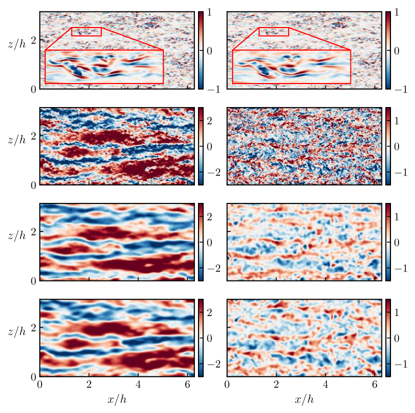
(a)(b)(c)(d)(e)(f)(g)(h)

Figure 2: (a,b) Snapshots of S1000 at $y^{+}=10$. (a) $v^{+}$. (b) $(v^{\dagger})^{+}$. (c-h) F5300 at $y/h=0.1$. (c) $u^{+}$. (d) $v^{+}$. (e) $(u^{\dagger})^{+}$. (f) $(v^{\dagger})^{+}$. (g) $u_{G}^{+}$, filtered with (10) and $\Delta_{x}\times\Delta_{z}=(4\times 2)y$. (h) $v_{G}^{+}$ with $(2\times 2)y$.

We use the methodology just described to generate flow reconstructions for all the cases in table 1. First, we tested if reconstructing fields ‘in-sample’ made a difference over reconstructing fields ‘out-of-sample’. For this purpose, we computed the operators for S1000 and F2000 using only half of the available velocitity fields. The correlations can be symmetrised, effectively multipliying by four the number of independent samples [21]. Thus, the linear operator converges reasonably fast and, no difference can be found between the in-sample and out-of-sample snapshots. Considering the outcome of this experiment, we use all the flow fields available to compute the correlations in (7).

Figure 2(a,b) shows snapshots of the true and reconstructed wall-normal velocity very close to the wall $(y^{+}\approx 10)$ in S1000. The reconstructed field captures the original in almost full detail, and the same is true for the other two velocity components, and for the Reynolds product $u^{\dagger}v^{\dagger}$ (not shown).

A similar level of accuracy only holds for $y^{+}\lesssim 20$. Figures 2(c-h) compare the true $u$ and $v$ with their reconstructions in the logarithmic layer $(y/h=0.1,\,y^{+}\approx 500)$. At this distance from the wall, most eddies with sizes smaller than $O(y)$ are missing from the reconstructions in figure 2(e,f). This agrees with the idea that ‘detached’ structures do not leave a footprint at the wall, and cannot be reconstructed from wall information. However, it is clear from the comparison of figures 2(e,f) and 2(c,d) that some large-scale information survives the reconstruction. This is best seen by comparing the reconstructed fields with those in figure 2(g,h), where the true velocities have been filtered with a low-pass Gaussian kernel,

$$G(x,y,z)=\left(\frac{2\pi}{\Delta_{x}\Delta_{z}}\right)^{1/2}\,\exp\left[-(\pi x/\Delta_{x})^{2}-(\pi z/\Delta_{z})^{2}\right],$$ (10)

where the filter widths are empirically adjusted to retain those large scales for which the error in the reconstruction is less than $50\%$. Figure 2 shows that, even far from the wall, the wall-normal velocity is organised into streaks. The reconstructed velocity fields include streaks of $u$, which account for most of the kinetic energy, and weaker $v$ structures of similar size. The energy of the latter is only about 10% of the total $v^{2}$-energy at that height, but their correlation with $u$ is strong enough for the reconstructed velocity field at the height of figure 2(c-h) to contain approximately $52\%$ of the tangential Reynolds stress. The filtered fields hold a similar amount of Reynolds stress, $45\%$, reinforcing the visual confirmation that the filter widths used are reasonable. The fair amount of Reynolds stress captured is not surprising if we consider that the spectral structure parameter, $-\phi_{uv}/(\phi_{uu}\phi_{vv})^{1/2}$, is known to be very close to unity for those large modes [22]. The long $v$ structures seen in the figure are those responsible for ‘lifting’ and maintaining the streaks [23].

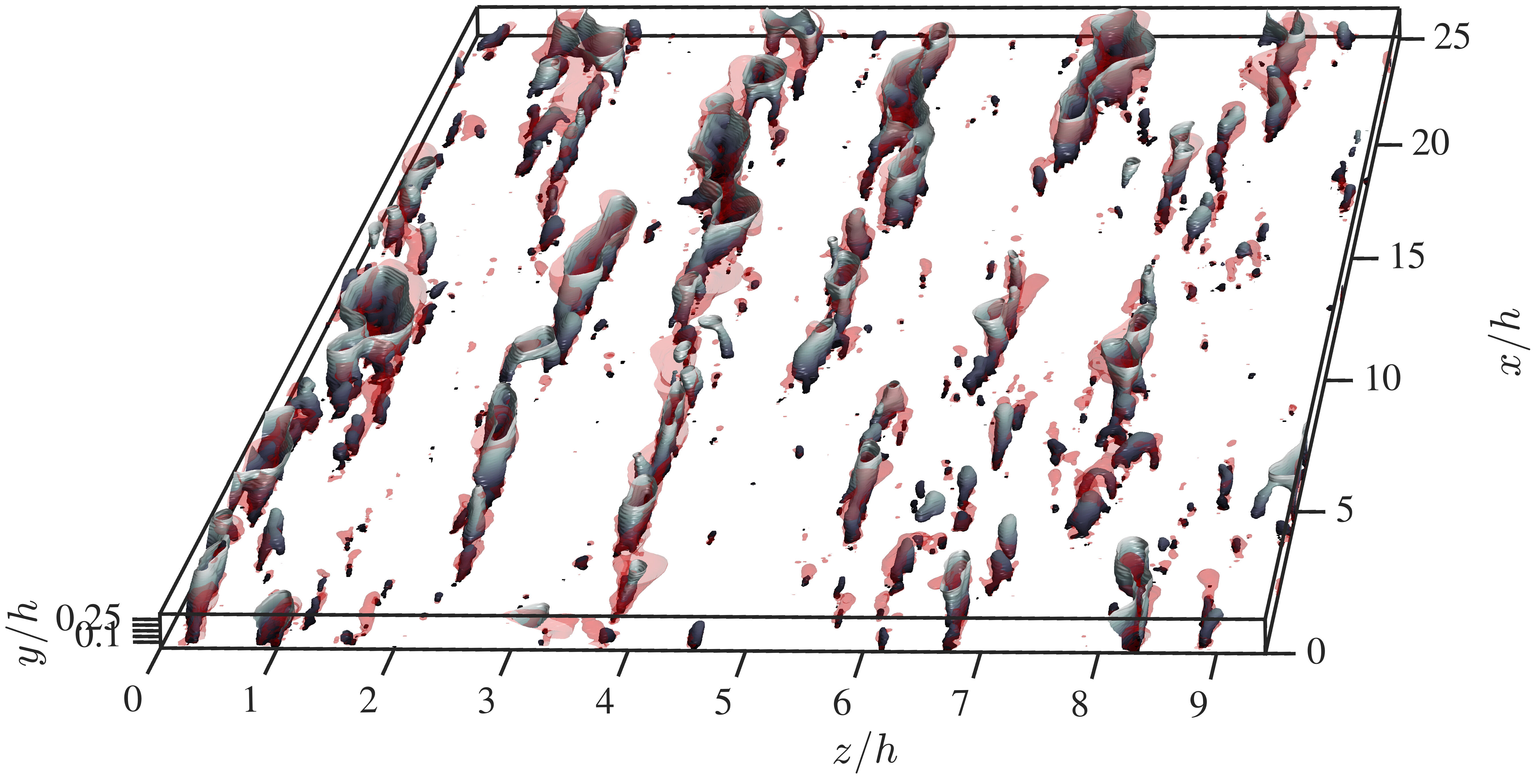
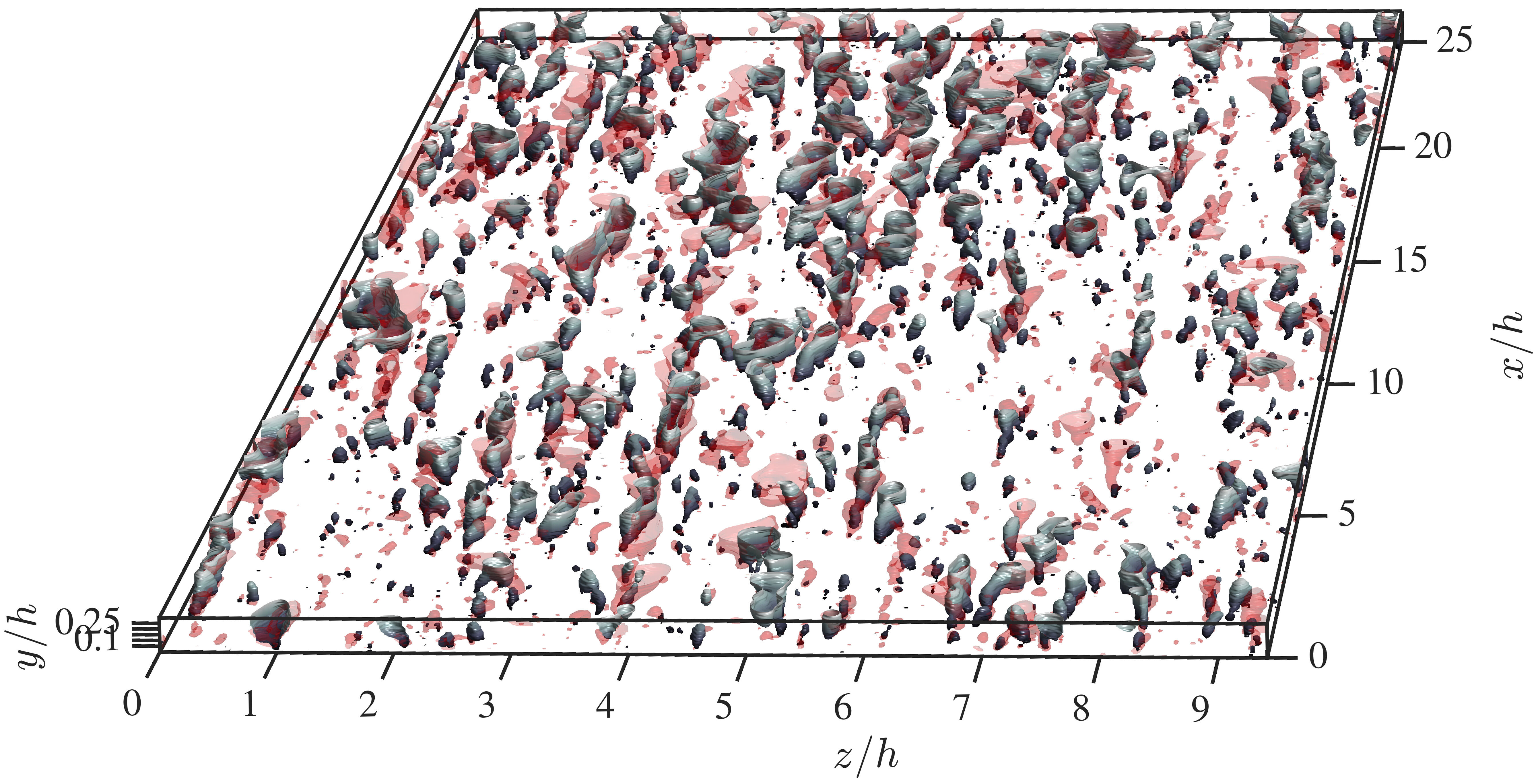
(a) (b)

Figure 3: Snapshot of the F5300 reconstruction. (a) The solid grey isosurfaces are $u^{\dagger}/u^{\dagger\prime}(y)<-1.5$, coloured with the distance from the wall, and the translucent red ones are $u_{G}/u_{G}^{\prime}(y)<-1.5$. (b) The solid grey isosurfaces are $u^{\dagger}v^{\dagger}/(u^{\dagger}v^{\dagger})^{\prime}(y)<-1.5$, coloured with the distance from the wall, and the translucent red ones are $u_{G}v_{G}/(u_{G}v_{G})^{\prime}(y)<-1.5$. The real velocities $u$ and $v$ (but not $u^{\dagger}$ and $v^{\dagger}$) are filtered using (10) with $\Delta_{x}\times\Delta_{z}=(4\times 2)y$ and $\Delta_{x}\times\Delta_{z}=(2\times 2)y$, respectively.

The relation between the two velocity components is even clearer in figure 3, which shows an instantaneous three-dimensional representation of the reconstructed velocity field below $y/h=0.25$. The solid grey isosurfaces of figure 3(a) represent the low-speed streaks of $u^{\dagger}$, while the red translucent ones are those of $u$. The original field has been filtered with (10) to retain only reconstructible scales. It is clear that, except for some discrepancies in the smaller structures far from the wall, all of the large features of $u$, including short or ‘broken’ streaks, are well reproduced. Most interesting are the isosurfaces of $-u^{\dagger}v^{\dagger}$, represented in solid grey in figure 3(b). As mentioned above, the reconstruction of $v$ is poor at this wall distance, but it is clear from the figure that the $v$-structures that can be reconstructed are those associated with intense Reynolds stress. The isosurfaces of in the figure are the ‘ejections’ and ‘sweeps’ [$Q_{2-4}$, 24, 25], which are known to mostly occur within the streamwise velocity streaks, and this arrangement is well captured by the reconstruction. Except for several ‘detached’ structures from the wall, most of the filtered Reynolds stress $Q_{2-4}$ structures that extend from the wall are well captured, and they are known to carry half of the total Reynolds stress [26].

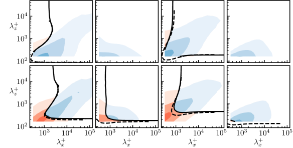
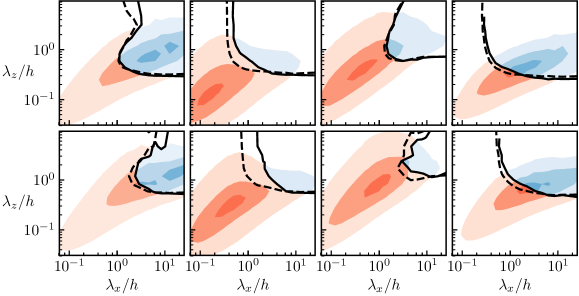
Figure 4: Spectral reconstruction error at different heights and Reynolds numbers, on top of the premultiplied velocity spectra and cospectrum(shaded) for F5300. The line contours are $R_{ab}=0.5$:            F2000;   , F5300. The shaded contours contain $90\%,50\%$ and $10\%$ of the total energy or of the tangential Reynolds stress. From left to right, $k_{x}k_{z}\phi_{uu}$, $k_{x}k_{z}\phi_{vv}$, $k_{x}k_{z}\phi_{ww}$ and $-k_{x}k_{z}\phi_{uv}$. From top to bottom $y^{+}\approx 20$, $y^{+}\approx 40$, $y/h=0.1$, $y/h=0.2$. The blue-shaded portion of the spectra marks the region reproduced with less than $50\%$ error.

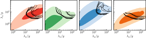
(a)(b)(c)(d) (e)(f)(g)(h)

Figure 5: Scaling of the error isolines with the distance from the wall for F5300. From left to right, $R_{uu}$, $R_{vv}$, $R_{ww}$, $R_{uv}$. (a-d) Wavelengths scaled with the channel height. Contours are $R_{ab}=0.5$ at $y/h=[0.012,0.025,0.05,0.1,0.15,0.2,0.3]$. The solid lines are within the logarithmic region, $150\nu/u_{\tau}<y\leq 0.2h$. (e-h) Wavelengths scaled with the distance from the wall, including only data within the logarithmic layer. Solid isolines, $R_{ab}=0.5$; dashed, $R_{ab}=0.25$; Shaded contours are the premultiplied spectra and cospectrum at $y/h=0.1$.

To quantify the performance of the reconstruction as a function of eddy size, we define the fractional spectral error

$$R_{ab}(k_{x},y,k_{z})=\dfrac{{\rm Re}\left\langle\left(a-a^{\dagger}\right)\left(b-b^{\dagger}\right)^{*}\right\rangle(k_{x},y,k_{z})}{{\rm Re}\langle ab^{*}\rangle(k_{x},y,k_{z})},$$ (11)

where $a$ and $b$ stand for either $u$, $v$ or $w$. The spectral error as defined above is related to other measures of correlation or ‘coherence’ across wall distances. Other works using LSE evaluate its performance using the Linear Coherence Spectrum [20, 7, 27],

$$\gamma^{2}_{ab}(k_{x},y,k_{z})=\dfrac{{\rm Re}\left\langle a^{\dagger}(b^{\dagger})^{*}\right\rangle(k_{x},y,k_{z})}{{\rm Re}\langle ab^{*}\rangle(k_{x},y,k_{z})},$$ (12)

which is related to $R_{ab}$ by,

$$R_{ab}=1+\frac{{\rm Re}\langle a^{\dagger}(b^{\dagger})^{*}\rangle}{{\rm Re}\langle ab^{*}\rangle}-2\gamma^{2}.$$ (13)

It follows from (13) that the greater the coherence, the lower the reconstruction error. For the limiting cases where the reconstruction error $R_{ab}$ is either unity or zero, both quantities are complementary, i.e. if the coherence is one, the error is zero and vice versa. One potential advantage of the spectral error is that the second factor in (13) penalises reconstructed energy without coherence, which may be significant for methods that are not $L_{2}$-optimal.

The contour of $R_{ab}=0.5$ is plotted at four wall distances in figure 4, compared with the energy spectrum of the three velocity components, and with the cospectrum of the tangential Reynolds stress. The regions shaded in blue and red indicate $R_{ab}<0.5$ and $R_{ab}>0.5$, respectively. In the first row, corresponding to $y^{+}=20$, the low-error region encloses most of the spectral plane and accounts for most of the energy, especially for $v$. As we saw in figure 2(a,b) the full flow field is well reconstructed at this distance from the wall. The accuracy decays quickly with $y$, especially for $w$. At $y^{+}=40$ (corresponding to the second row), the $R_{ww}=0.5$ isoline only encloses wavelengths two to three times longer and wider than those at $y^{+}=20$. Figure 4 contains data at two Reynolds numbers. At the wall distances in the first two rows, which are in the buffer layer, the error isolines collapse well in wall units. In this range, the widest reconstructible spectral range is that of $v$, but, because the large scales of $v$ contain much less energy than those of $u$, the latter is the best reproduced variable in terms of energy. These relations persist up to $y^{+}\approx 60$.

The trend to poorer reconstruction for larger $y$ persists as we move into the logarithmic layer, as shown by the last two rows in figure 4. They are normalised in outer units and also collapse reasonably well for the two Reynolds numbers in the figure. The spectral region that can be well reconstructed is different for the four variables. In general, $w^{\dagger}$ has the narrowest spectral range, and $v^{\dagger}$ and $u^{\dagger}v^{\dagger}$ the widest one, although it is interesting that the Reynolds product, $u^{\dagger}v^{\dagger}$, can be reconstructed over a wider range that either $u^{\dagger}$ or $v^{\dagger}$. Note that the spectral error only makes sense within the non-zero part of the spectra, since otherwise (11) is essentially undetermined.

The wavelengths of the error isolines above the buffer layer are approximately proportional to their distance from the wall, confirming that the eddies that are ‘attached’ in this sense are self-similar [1]. This is illustrated in figure 5, where the reconstruction boundaries are shown at different heights, scaled both with $h$ and with $y$. The good scaling with $y$ is evident in the lower row of figures. The spanwise dimensions of the reconstructed $u^{\dagger}$, $v^{\dagger}$, and $u^{\dagger}v^{\dagger}$ are $\lambda_{z}\gtrsim 2y$, which is in fair agreement with the dimensions of the attached ‘quadrant’ (Q-)eddies isolated in the logarithmic region by thresholding $uv$ [28]. The streamwise scales that can be reconstructed differ among variables. The longest one is $u^{\dagger}$, probably because the shorter features of $u$ are less energetic, but $v^{\dagger}$ and $u^{\dagger}v^{\dagger}$ can be reconstructed down to $\lambda_{x}\approx 5y$, which is again in reasonable agreement with the dimension of Q-structures in [28]. In any case, while the relation between different variables appears robust, the absolute limits should not be taken too seriously. The 25% error isolines in the lower row of figure 5 show that the limits depend on the chosen error threshold.

As mentioned above, the spanwise velocity component is the worst reproduced at all heights. As seen in figures 4 and 5, its wavelength range is approximately 40% smaller than for $u$ or $v$, although it is interesting to note that the instantaneous reconstructed fields satisfy continuity everywhere [13]. Even though the observable wavelengths of $w$ are limited to longer (and wider) scales than those of $v$, the reconstructions of both velocity components contain similar kinetic energy, as these scales of $w$ are more energetic than the large scales of $v$. We will see below that $w$ is mostly associated with the shear at the wall, suggesting streamwise rollers or vortices. If this were instead the case, each roller would have a lower and an upper layer of $w$ and, while the lower layer would leave a clear wall footprint, the upper one would be harder to reconstruct.

Figure 6 compares the overall performance of the reconstructions by means of the ratio

$$\beta_{ab}(y)=\frac{\sum_{\forall k_{x},k_{z}}a^{\dagger}(b^{\dagger})^{*}(k_{x},y,k_{z})}{\sum_{\forall k_{x},k_{z}}ab^{*}(k_{x},y,k_{z})},$$ (14)

between the energy of the reconstructed and original fields. The solid lines in the figure show that reconstruction recovers more than 50% of $u^{2}$ and $uv$ below $y/h\approx 0.2$, but that the cross-flow velocities are only reconstructed to that accuracy within the buffer layer, $y^{+}\lesssim 100$. All the reconstructions degrade above $y/h\approx$0.2-0.3.

IV.1 Incomplete wall data

Not all observables contribute equally to the reconstruction. Their relative contribution is different for each velocity component, and changes between the buffer and the logarithmic layer. In this section, we explore these differences by repeating the previous study using only one observable at a time, as detailed in the discussion of (6). The restricted reconstructed velocity fields are denoted as ${a}^{\dagger}_{p}$, ${a}^{\dagger}_{u_{y}}$ and ${a}^{\dagger}_{w_{y}}$, where $a$ stands for the variable being estimated, and the subindex is the observable.

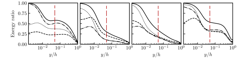
(a)(b)(c)(d)
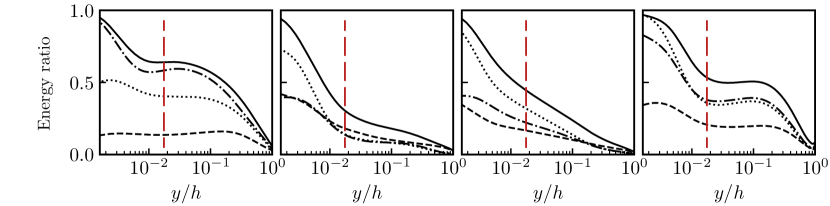
(e)(f)(g)(h)

Figure 6: Reconstructed energy ratio with single-observable models for F2000 (top) and F5300 (bottom). The lines are:   , ${a}^{\dagger}$;                   , ${a}^{\dagger}_{u_{y}}$;            ${a}^{\dagger}_{w_{y}}$;            , ${a}^{\dagger}_{p}$. From left to right, $uu$, $vv$, $ww$, $uv$. The dashed vertical lines are $y^{+}\approx 100$, approximately corresponding to the end of the buffer layer.

Figure 6 compares the performance of the different restricted reconstructions with that of the full model. The reconstruction with the highest energy fraction is $u^{\dagger}$. Not surprisingly, the most important observable is $\partial_{y}u$ in this case, and $u^{\dagger}_{u_{y}}$ closely approximates the full model. The spanwise shear, and especially the pressure, have much less influence on this component. On the other hand, $v$ is, on average, mostly reconstructed from the pressure, which seems reasonable, except very near the wall, where the spanwise shear dominates. This is probably associated with the presence of the near-wall streamwise vortices. The correlation between the wall pressure and $v$ was studied in some detail by [14]. They find that the correlation is almost always maximum at zero spanwise offset, but that it has weak side-lobes at $\Delta z^{+}\approx\pm 50$ when $v$ is in the buffer region, consistent with the known structure of the streamwise vorticity in the sublayer [29]. The spanwise velocity is mostly controlled by the spanwise shear near the wall, but all observables have a similar influence on it farther away. As we have already discussed, the reconstruction of this variable is generally poor.

On the other hand, the tangential Reynolds stress, $u^{\dagger}v^{\dagger}$, is fairly well reconstructed up to $y/h\approx 0.3$. It is intriguing that $u^{\dagger}v^{\dagger}$, behaves better than $v^{\dagger}$, which is one of its factors, but we already mentioned when discussing figure 3 that the reason is that the large $v$-structures that can be reconstructed from the wall are precisely those associated with the large streaks of the streamwise velocity. The relevant observables for $u^{\dagger}v^{\dagger}$ are intermediate between those for $u^{\dagger}$ and $v^{\dagger}$. In the buffer layer, the two shears are dominant, while the pressure is not. Farther away from the wall, the three observables are comparable. Note that the good behaviour of this variable is encouraging from the point of view of observing dynamics from the wall.

The reconstructions for the two Reynolds numbers agree reasonably well in inner units close to the wall $(y^{+}<100)$, and in outer units far from it. The obvious exception are the reconstructions based only on the pressure in figure 6, which contain considerably less energy at the higher Reynolds number. This trend is most pronounced for $u^{\dagger}_{p}$ and, consequently, for $u^{\dagger}_{p}v^{\dagger}_{p}$, for which the reconstructed energy is 50% smaller for F5300 than for F2000. The degradation is restricted to the reconstruction from the pressure, and does not affect either the full model or the reconstructions in terms of the shears. Inspection of the spectra of $u^{\dagger}_{p}$ and $v^{\dagger}_{p}$ at the two Reynolds numbers reveals that most of the energy missing from F5300 resides in relatively elongated scales, which we will see below to be dominated in the full model by the shear (see figure 7). A possible explanation for this behaviour follows from the decomposition of the pressure at the wall into an ‘inertial’ component,

$$\nabla^{2}p_{I}=-\nabla\cdot(u\cdot\nabla u),\qquad\partial_{y}p_{I}\big{|}_{y=0}=0,$$ (15)

and a ‘Stokes’ one [30],

$$\nabla^{2}p_{s}=0,\qquad\partial_{y}p_{s}\big{|}_{y=0}=\nu\partial_{yy}v,$$ (16)

Encinar et al. [15] showed that the latter can be computed from the wall shears using continuity,

$$\widehat{p}^{+}_{s}(0)=-{\rm i}\left[k_{x}^{+}\widehat{u}_{y}(0)^{+}+k_{z}^{+}\widehat{w}_{y}(0)^{+}\right]/|k|^{+}.$$ (17)

It can be shown that the ratio of between $\widehat{p}_{s}$ and $\widehat{p}_{I}$ is approximately independent of the Reynolds number when the wavenumbers are scaled in wall units, but that it decays as $\lambda^{+}_{x}$ increases along the diagonal $\lambda_{z}=\lambda_{x}$, which contains the cores of the velocity spectra (see figure 7), essentially because $k_{x}k_{z}\phi_{pp}(0)$ is located along this diagonal, but the two shears are not (figure 1b). The result is that, as $Re_{\tau}$ increases and we use our estimation to reconstruct $u^{\dagger}_{p}$ at a fixed $y/h$, and therefore at increasing $\lambda^{+}_{x}\sim y^{+}=Re_{\tau}y/h$, the importance of the Stokes component decreases. It follows from (17), that $p_{s}$ is actually part of the shears, but there is no reason why the particular combinations of shears in (17) is in any way optimal to reconstruct the velocities. The pressure-only reconstructions are therefore contaminated by $p_{s}$, and should asymptote to a ‘pure’ reconstruction in terms of $p_{I}$ as $Re_{\tau}$ increases. In this view, the ‘purest’ $u^{\dagger}_{p}$ is the one for F5300, and the apparently higher energy fraction in F2000 is accidental. The full model does not have this problem, because it uses information from the two shears to compensate the spurious effect of $p_{s}$. As a consequence, its performance in figure 6 does not change with $Re_{\tau}$.

Figure 6 is contaminated below $y^{+}\approx 100$ (indicated by a vertical red line) by the relatively low resolution of the data stored for F2000 and F5300, and we used the higher-resolution smaller box S1000 to estimate the effect of the contamination. The only difference found was a better performance of $v^{\dagger}_{p}$ and $w^{\dagger}_{p}$ (but not of $u^{\dagger}_{p}$), most probably because of a better estimation of the streamwise vortices of the buffer layer. This idea is supported by the high value of the cross-correlation between $w_{y}$ and $p$ at the wall, which is close to unity for the small scales, and the fact that $w_{y}$ is the best predictor of the cross velocities in the buffer region.

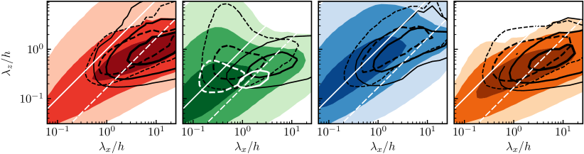
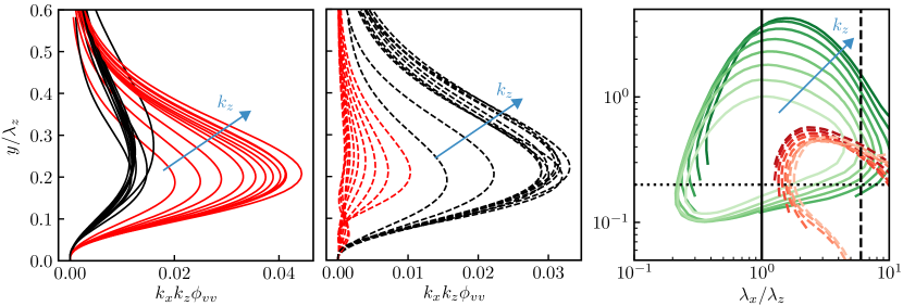
(a)(b)(c)(d) (e)(f)(g)

Figure 7: (a-d) Premultiplied spectra and cospectrum at $y/h=0.1$ for F5300. Shaded, spectrum of the original fields;   , spectrum of the reconstruction using only the streamwise shear;            , using only the pressure. The contour levels for all the spectra are 1.5%, 10% and 50% of the maximum of the corresponding true spectrum. The white contours in (b) are reconstructions at $y/h=0.05$. The diagonal lines are:   , $\lambda_{x}=\lambda_{z}$;            , $\lambda_{x}=6\lambda_{z}$. (a) $k_{x}k_{z}\phi_{uu}$. (b) $k_{x}k_{z}\phi_{vv}$. (c) $k_{x}k_{z}\phi_{ww}$. (d) $-k_{x}k_{z}\phi_{uv}$. (e-f) Premultiplied spectra of $v^{\dagger}_{p}$ (red) and $v^{\dagger}_{u_{y}}$ (black). (e) Modes along $\lambda_{x}=\lambda_{z}$. (f) Along $\lambda_{x}=6\lambda_{z}$. (g) Streamwise sections at different $\lambda_{z}\in(0.1-0.84)$, from dark to light, of:   , $k_{x}k_{z}\phi_{vv}^{+}=0.05$;            , $k_{x}k_{z}\phi_{uu}^{+}=0.3$. The straight lines are,   , $\lambda_{x}=\lambda_{z}$;            , $\lambda_{x}=6\lambda_{z}$;            , $y=0.2\lambda_{z}$.

Figure 7(a-d) displays the spectral distribution of the energy reconstructed by the different single observables. In most cases, the wall pressure and the two shears predict similar spectral regions, comparable to those of the the full reconstructions in figure 5, but the behaviour of $v^{\dagger}$ in the logarithmic layer is interesting, because different observables dominate in different spectral ranges.

The spectrum of $v$ has a wide and a narrow component in the logarithmic layer [31], which appear in figure 7(b) as the two ‘horns’ on the upper right-hand corner of the spectrum. The spanwise wall shear contributes most to the estimation of the longer component, and the pressure dominates the shorter one, suggesting, respectively, streamwise rollers and compact sweeps and ejections. The reconstruction from the pressure is centred on equilateral wavenumbers, whereas the reconstruction from the streamwise shear dominates at wavelengths elongated in the streamwise direction. Only $v^{\dagger}_{u_{y}}$ is shown in figure 7, but the effect on $v^{\dagger}$ of the two shears is similar above $y^{+}\approx 100$.

That this separation among $v$-structures is not restricted to a particular distance from the wall is shown in figure 7(e,f), which displays profiles of the energy spectrum of $v^{\dagger}_{p}$, in red, and of $v^{\dagger}_{u_{y}}$, in black, at various points along the two diagonals in figure 7(b). Along the equilateral solid diagonal for which the pressure reconstruction is dominant, $\lambda_{x}=\lambda_{z}$, the spectrum reconstructed from the pressure is approximately three times more intense than that of $v^{\dagger}_{u_{y}}$ (figure 7e), and the opposite is true for the longer structures in figure 7(f), $\lambda_{x}=6\lambda_{z}$. It is interesting that the peak of the reconstructed spectra is at $y/\lambda_{z}\approx 0.2$ for all the wavelengths for which this peak is in the logarithmic layer. When a similar plot is drawn for the true $v$, the peak is at $y/\lambda_{z}\approx 0.3-0.5$. Reconstruction from either observable only recovers structures closer to the wall than the average for the real flow field, presumably corresponding to the ‘roots’ of taller attached eddies.

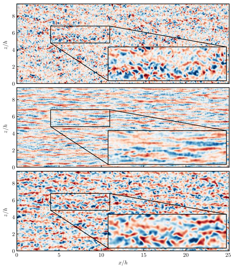
Figure 8: Reconstruction of the wall-normal velocity at $y/h=0.1$ in F5300. Top, using only the pressure, $v^{\dagger}_{p}$. Middle, using only the wall shear, $v^{\dagger}_{u_{y}}$. Bottom, true velocity field, filtered with (10) and $\Delta_{x}\times\Delta_{z}(2\times 2)y$. The shading goes from $-u_{\tau}$ to $u_{\tau}$.

Further insight into the difference among the two reconstructions is provided by figure 7(g), which contains streamwise sections of the premultiplied spectrum of $u$, in red, and of $v$, in green; represented against the wavenumber aspect ratio. The reconstruction peak at $y/\lambda_{z}=0.2$ is marked by the horizontal dotted line, and intersects the lower edge of the $v$-spectrum. The two diagonals in figure 7(b) are represented by vertical lines in this plot, as they contain wave numbers with constant aspect ratio. The solid vertical line is the equilateral diagonal, and crosses the centre of the $v$-spectrum. This is the spectral location at which $v^{\dagger}$ is best reconstructed by the wall pressure, and figure 7(g) suggests that it contains $v$-structures whose lower edge interacts with the impermeability of the wall to create a pressure peak, as larger modes are damped faster when they approach the wall. In contrast, the elongated diagonal $\lambda_{x}=6\lambda_{z}$, represented in the figure by the dashed vertical line, crosses the peak reconstruction wall distance at the edge of the $v$-spectrum, but near the centre of the spectrum of $u$. This $v$-structures are too far from the wall to create an overpressure, but they can be detected from the wall shear because they are associated with the streaks of $u$, whose spectrum reaches the wall in this region. Finally, figure 8 displays two $v^{\dagger}$ snapshots reconstructed from the pressure (top), and from the wall shear (bottom). The difference in geometry is obvious, and the lateral spacing between streaky $v$-structures of similar sign in the bottom snapshot $(\Delta z/h\approx 0.6,\Delta z^{+}\approx 3200)$ approximately agrees with the separation between the streamwise velocity streaks at the distance from the wall of the figure (see the spectrum in figure 7a). It is interesting that, although it follows from figure 6(h) that the total $uv$-energy reconstructed from the streamwise shear is approximately twice larger than the one reconstructed from the pressure, the tangential Reynolds stress contained in intense structures [28] of the two snapshots in figure 8 are approximately equal (not shown), with similar intensity and area fraction.

IV.2 Reconstruction in physical space

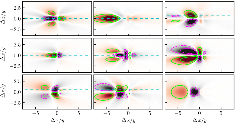
(a)(b)(c)(d)(e)(f)(g)(h)(i)

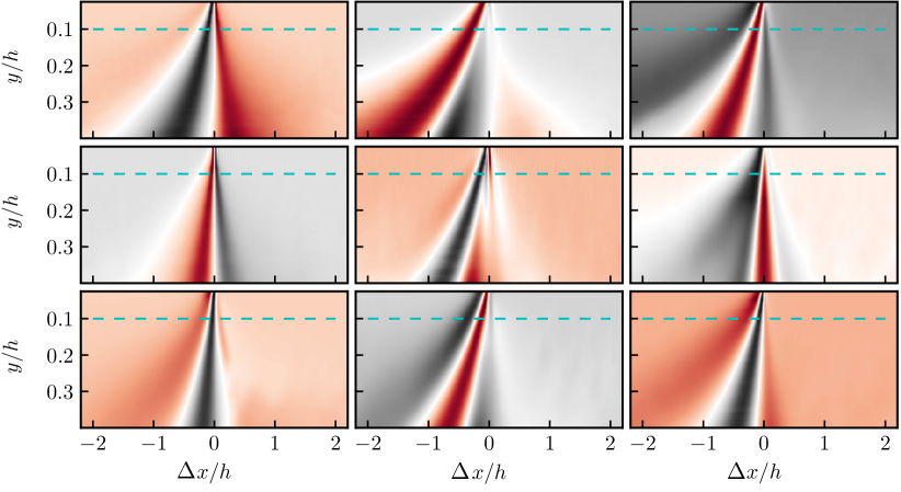
Figure 9: Components of the operator $\widetilde{L}_{s}$ for F5300. The rows are the operator for $u$, $v$ and $w$, from top to bottom. The columns are the components corresponding to $p$, $u_{y}$ and $w_{y}$, from left to right. Shaded contours are for $y/h=0.1$, positive in red and negative in black. Lines are for $y/h=0.05$, positive in green and negative in magenta. The contour levels are $[-0.5,-0.2,0.2,0.5]$ of the maximum absolute value at each height. The dashed lines indicate the vertical sections in figure 10.

(a)(b)(c)(d)(e)(f)(g)(h)(i)

Figure 10: As in figure 10. Streamwise sections: $z=0$ for symmetric components, and at the location of the maximum absolute value at each height for antisymmetric ones. The dashed line is $y/h=0.1$. The shading is scaled with the maximum absolute value at each height.

Although the spectral expression of the reconstruction operator discussed in the previous section is very useful in understanding the behaviour of the different flow scales, its physical-space counterpart defined in (8) and (9) gives a more intuitive representation of the operation that is actually being performed. It is probably also easier to generalise to wall-bounded flows besides the channel. We saw in §III that the LSE operator is essentially a two-point correlation scaled with the cross-correlation tensor of the observables at the wall, and both correlations are likely to be reasonably independent of the type of flow in the near-wall region where the reconstruction is effective. For example, this is the case for boundary layers and channels below $y/h\approx 0.1$, although they differ farther from the wall [32].

Figures 10 and 10 show sections of the physical-space reconstruction operator $\widetilde{L}_{s}^{(a)}$ for the three velocity components, $a=\{u,v,w\}$, and the three observables, $s=\{p,u_{y},w_{y}\}$. Note that, although $\widetilde{L}$ is formally a function of the two wall-parallel coordinate increments, $\Delta x=x-x^{\prime}$ and $\Delta z=z-z^{\prime}$, and of the reconstruction height $y$, their role is different. The operator is always two-dimensional in $(\Delta x,\Delta z)$, and acts as a convolution kernel on $E(x^{\prime},z^{\prime})$ at the wall. The wall-normal coordinate $y$ is a parameter, and the operators for the reconstruction at different wall distances are, in principle, unrelated to each other. To emphasise this, the coordinates in these two figures have been inverted. The operator for one wall distance is given by the section of the three-dimensional function $\widetilde{L}(\Delta x,y,\Delta z)$ at one $y$, as in figure 10, and $\Delta x<0$ implies that the convolution kernel is acting on the wall upstream of the reconstruction point.

The wall-parallel reconstruction kernels in figure 10 show that the main reason for the lack of small scales in the reconstructions is that operators act as smoothing filters. All kernels have positive and negative parts, and their relative arrangement can partly be predicted from symmetry considerations. For example, $\widetilde{L}^{(u)}_{u_{y}}$ in figure 10(b) is symmetric with respect to $\Delta z=0$ because both $u$ and $u_{y}$ are symmetric with respect to $\Delta z\to-\Delta z$, but $\widetilde{L}^{(u)}_{w_{y}}$ in figure 10(c) is antisymmetric because $u$ is symmetric and $w_{y}$ is antisymmetric. This has to be taken into account in interpreting figure 10, because the shape of some of the kernels suggests that the relevant variable is not the observable but some of its derivatives. For example, the positive-negative alternation along the $\Delta x$ axis, centred at $\Delta x=0$, of $\widetilde{L}^{(u)}_{p}$ in figure 10(a) probably implies that the relevant observable is not $p$ but $\partial_{x}p$, because there is no statistical symmetry to $\Delta x\to-\Delta x$, and thus $\widetilde{L}^{(u)}_{\partial_{x}p}$ should be maximum at $\Delta x=0$. A similar argument can be made from the Fourier counterpart of (6), which, for a single Fourier mode is

$$\langle\hat{p}^{*}\hat{p}\rangle\hat{L}^{(u)}_{p}=\langle\hat{p}^{*}\hat{u}\rangle.$$ (18)

This equation is related to the one for the estimation of $u$ from $\widehat{\partial_{x}p}=ik_{x}\hat{p}$,

$$-k_{x}^{2}\langle\hat{p}^{*}\hat{p}\rangle\widehat{L}^{(u)}_{\partial_{x}p}=ik_{x}\langle\hat{p}^{*}\hat{u}\rangle,$$ (19)

which is identical to (18) except for a factor multiplying each side of the equation. The left-hand side its multiplied by $-k_{x}^{2}$, which is a even factor. This is the only possibility, because the first factor represents the autocorrelation of $\partial_{x}p$, which by definition is a symmetric function. On the other hand, the right-hand side gets multiplied by the odd factor $ik_{x}$, which implies that, for a dominantly skew-symmetric $\widetilde{L}^{(u)}_{p}$, such as the one in figure 10(a), the operator $\widetilde{L}^{(u)}_{\partial_{x}p}$ should be approximately symmetric along the streamwise direction, peaking at $\Delta x\approx 0$. The similar alternation in $\Delta z$, which would suggest $\partial_{zz}p$, may be due to the spurious symmetry of the correlation along the $\Delta z$ axis, and could equally be interpreted as a statistical distortion of $\partial_{z}p$ in which 50% of the events fall to either side of the reconstruction point. For a discussion of symmetry artifacts of LSE in the context of the local reconstruction of the buffer layer, see [33].

The evolution of the reconstruction kernels with the distance from the wall of the target point is displayed in figure 10. Symmetric kernels are plotted at the symmetry plane, $\Delta z=0$, but antisymmetric ones, for which this plane is identically zero, are plotted at the $\Delta z$ plane for which the kernel is most intense. A general property of all the kernels is that they become wider as $y$ increases, and that the growth is almost linear, suggesting self-similarity with respect to $y$. In fact, the wall-parallel plot in figure 10 is scaled with $y$, and includes two wall distances, whose kernels collapse well in this representation. Another property of most kernels in figure 10 is that they tilt forward, implying that the flow is reconstructed from upstream wall variables. Reference [14] found that the correlation of $v$ with the pressure at the wall is antisymmetric in $\Delta x$, with both upstream and downstream lobes, but figure 10(d) shows that the corresponding kernel, $L^{(v)}_{p}$, is one of the few that is not tilted in $\Delta x$. This approximately applies to all the kernels based on the wall pressure, but those based on the shears are tilted by an angle that depends on the particular case, but which is of the order of 10^o–20^o to the wall, similar to other structural angles measured for $u$ and $w$ in the logarithmic layer of shear flows [32]. The disparity between the tilting of the shear and pressure kernels can be explained if we consider the processes generating the signals at the wall. If an attached eddy of size $O(l)$ is centred at a distance to the wall of $y_{l}\sim l$, the time it takes for a change of its dynamics to affect the shear at the wall should be of the order of $t_{l}\sim y_{l}/u_{\tau}\sim l/u_{\tau}$, equivalent to his local turnover time. Coincidentally, this time is related to the shear time by the Corrsin shear parameter, which is of the order of 10 for the logarithmic region of channel flows [2]. This implies that the eddy is advected downstream during the time it takes for the information to reach the wall. In contrast to that, the pressure of incompressible fluids instantly transmits sudden changes globally, generating a signal at the wall with no offset.

IV.3 Off-design behaviour

Although the reconstruction operators are Re-dependant, they are obtained from two-point correlation tensors which are known to collapse in inner units close to the wall, and in outer units farther away [32]. This scaling extends to the linear estimators, allowing operators developed from DNS to be used at a different Reynolds number than the one at which they were obtained. Figure 11(a,b) presents a snapshot of the true $v$ and of the reconstructed $v^{\dagger}$ in the buffer layer of S2000, and figure 11(c) presents a similar reconstruction of $u$ in the logarithmic layer. Both reconstructions are performed using an operator computed from S1000. For the buffer-layer reconstruction $(y^{+}\approx 10)$, the observables, velocities and operators have been scaled in inner units, and, for the logarithmic region $(y/h\approx 0.1)$ they have been scaled in outer units. Although there is some degradation of accuracy with respect to the reconstructions at the nominal Reynolds number in figure 2, the result is still reasonable. The worst errors are in scales that are not contained in the rescaled operators. For example, for computational boxes with similar dimensions in outer units, operators obtained at lower Reynolds numbers lack some of the longest scales when scaled in wall units. Similarly, some of the smallest scales are missing from those operators when scaled in outer units. The reconstructions in figure 11(b,c) have been correspondingly mildly filtered to avoid aliasing artefacts. The reconstruction operators are models of the structure of the flow, and the success of the rescaling supports the intuition that the attached turbulent structures near and far from the wall approximately scale in inner and outer units, respectively.

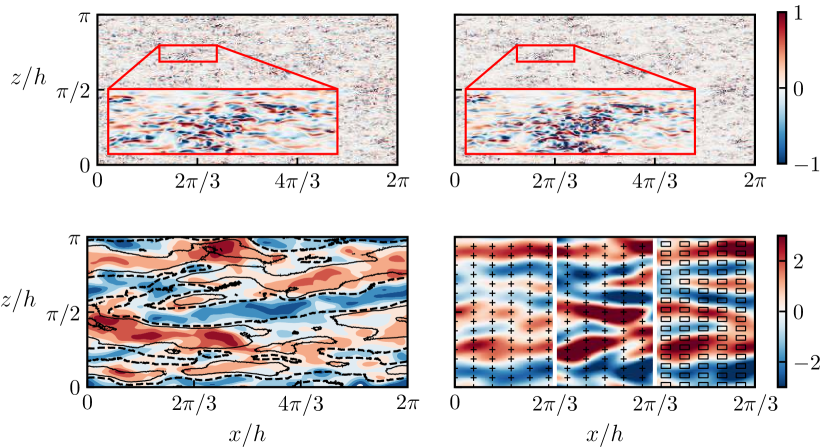
(a)(b)(c)(d)(e)(f)

Figure 11: Snapshots of different reconstructions. (a) S2000, $v^{+}$ at $y^{+}\approx 10$. (b) S2000, $(v^{\dagger}_{\text{S1000}})^{+}$ at $y^{+}\approx 10$. (c) S2000 at $y/h\approx 0.1$. Shaded, $u^{+}$; ——, $(u^{\dagger}_{\text{S1000}})^{+}=1$;            , $(u^{\dagger}_{\text{S1000}})^{+}=-1$. S2000 is filtered with $G$ and $\Delta_{x}\times\Delta_{z}=(0.4\times 0.2)$. (d-f) S1000, $(u^{\dagger})^{+}$ at $y/h\approx 0.1$, with information limited to discrete sensors (black crosses). (d) Fully dealiased. (e) No dealiasing. (f) Sensors averaged over 25% of the wall surface.

IV.4 Practical application with limited input data

Lastly, we explore some of the issues pertaining to the practical application of this methodology. Figure 11(d-f) shows $u^{\dagger}$ at $y/h=0.1$ for S1000, reconstructed from wall observations which are assumed to be only known at a coarse grid of sensors spaced by $\Delta_{x}/h=0.2$ and $\Delta_{z}/h=0.1$, represented in the figure by black crosses. Sampling has the effect of limiting the spatial resolution of the observables to wavelengths longer than the Nyquist limit $(2\Delta_{x},2\Delta_{z})$, and of aliasing the information of the shorter wavelengths into longer ones that fall within this limit [34]. If the information can be properly dealiased by filtering the short wavelengths before sampling, the only effect is the loss of resolution, as in figure 11(d). Because of the linearity of the reconstruction and the homogeneity in the wall-parallel planes, this is equivalent to a posteriori filtering of a reconstruction performed at full resolution. Unfortunately, this is usually impossible, because the full measurements are unavailable. Figure 11(e) shows the worst-case scenario in which ‘point’ sensors are used without dealiasing. The reconstruction is heavily distorted, mostly in the form of higher intensities, and the effect is more severe than what could be expected from simple aliasing of the wall observables. The reason is that the latter contain a lot of small scales which should have no effect on reconstructions far from the wall, but which are aliased into larger scales and amplified by the linear operator into large spurious features of the reconstruction. A more realistic scenario is presented in 11(f), in which the sensors are modelled as finite rectangles with size $\Delta_{x}/h=0.1$ and $\Delta_{z}/h=0.05$, and assumed to provide values averaged over their surface. This a priori filtering does not fully eliminate the aliasing error, but reduces it significantly by reducing the short-wavelength content of the wall observables. In a real experimental application, where the temporal evolution of the sensor signal is available, time filtering can also be used to limit the aliasing error. The lifetimes [17] and convection velocities [35] of the turbulent structures in the logarithmic layer are known, and are typically significantly longer and faster than those of the scales responsible for the aliasing of the wall signal. Time filtering of the signals at those scales mimics streamwise averaging through Taylor’s approximation, and supplements the benign effect of non-zero sensor size.

V Conclusions

We have shown that the three velocity components in turbulent channels can be reconstructed reasonably well below $y/h\approx 0.2$ with linear stochastic estimation, using only the observed pressure and the streamwise and spanwise shear at the wall. Only eddies attached in the sense of having sizes comparable to $y$ [36], are reconstructed, but these are found to contain more than approximately 50% of the kinetic energy of $u$, and of the tangential Reynolds stress, $uv$, in the logarithmic layer. The optimum reconstruction uses the three wall observables, but not all them are equally important, and the relative balance among them depends on the variable being reconstructed and on the distance from the wall. We have proposed that this can be used to sharpen the definition of which velocity components are attached to the wall in which spectral ranges, defining as attached those eddies that can be reconstructed from wall information, regardless of the particular reconstruction method. The results differ from the generally accepted ones in some cases. For example, the wall-normal velocity, which is usually considered a detached variable because it is inhibited near the wall by the impermeability condition, is linked to the wall by the pressure, for equilateral scales, and by the wall shears, for longer scales in which $v$ is associated with the $u$-streaks. Interestingly, although the two sets of attached $v$-structures defined in this way, are very different, with a different balance of $u$ and $v$ components, both are active in the sense of generating a comparable amount of tangential Reynolds stress.

Although most of the paper deals with mode-by-mode reconstructions in the Fourier representation of the flow, we have shown that the expressions of the operators in physical space gives interesting information on the flow physics. Thus, while the wall pressure predominately reconstructs velocities immediately above the the observation point, the effect of the shear is transmitted along lines inclined by 10^o–20^o from the wall, comparable to previous observations of the structures of $u$ and $w$ in wall-bounded flows.

We have also shown that the reconstruction operators obtained at one Reynolds number can be adapted to a different one by proper scaling, making them potentially useful for control strategies in which only wall observations are available, or, in turbulence physics, for the study of the flow dynamics from the wall. They can be adapted to experimental set-ups in which the instantaneous measurements are only available on a coarser grid of sensors, but only after careful dealiasing of the observations. Although not explicitly shown, it can be inferred from figure 6 that the information provided by the two shears is equivalent in the logarithmic region, and a practical grid of sensors may obviate the spanwise shear with almost no penalty in the accuracy of the reconstructions. Note that this does not apply to the flow in the buffer layer, where the spanwise shear is the most relevant observable for the cross flow.

The reconstruction operators for the four cases considered will be made available at https://torroja.dmt.upm.es/channels/data/.