Structured Semantic Model supported Deep Neural Network for Click-Through Rate Prediction

Abstract

With the rapid development of online advertising and recommendation systems, click-through rate prediction is expected to play an increasingly important role. Recently many DNN-based models which follow a similar Embedding&Multi-Layer Perceptron (MLP) paradigm, and have achieved good result in image/voice and nlp fields. Applying Embedding&MLP in click-through rate prediction is popularized by the Wide&Deep announced by Google. These models first map large scale sparse input features into low-dimensional vectors which are transformed to fixed-length vectors, then concatenated together before being fed into MLP to learn the non-linear relations among input features. The number of trainable variables normally grow dramatically as the number of feature fields and the embedding dimension grow. It is a big challenge to get state-of-the-art result through training deep neural network and embedding together, since it falls into local optimal or overfitting easily. In this paper, we propose an Structured Semantic Model (SSM) to tackle this challenge by designing an orthogonal base convolution and pooling model which adaptively learns the multi-scale base semantic representation between features supervised by the click label. The outputs of SSM are then used in the Wide&Deep for CTR prediction. Experiments on two public datasets as well as real Weibo production dataset with over 1 billion samples have demonstrated the effectiveness of our proposed approach with superior performance comparing to state-of-the-art methods.

1 Introduction

Click-through rate (CTR) is widely used in advertising and recommender systems to describe users’ preferences on items. For cost-per-click(CPC) advertising system, the revenue is determined by bid price and CTR. For recommender system, CTR is used to improve user experience. So it’s important to improve the performance of CTR prediction, and CTR prediction has received much attention from both academia and industry communities.

In recent years, DNN has been researched and applied with structured data for CTR prediction after gaining popularity of deep learning in image, voice, NLP, etc. fields.

Structured data is particularly abundant(such as user behavior data, blog segmentation, user interest, etc.) for CTR prediction, which requires a lot of feature engineering effort with traditional methods. DNN-based models can take advantages of those structured data and deep feature representation could be learned through embedding and multi-layer perceptrons. But it requires training large number of variables and using lots of training epochs which aggravates the risk of overfitting and dramatically increases the computation and storage cost, which might not be tolerated for an industrial online system.

There are many researches based on CNN, but due to the particularity of advertising/recommended data, there are no context data like images and voices. Therefore, the convolution and pooling over advertisement/recommended data is usually unexplainable.

In the field of search, Microsoft’s proposed DSSMHuang et al. (2013) model establish as supervised semantic model for doc and query, which learns the non-linear relations of word granularity well. Inspired by this, we propose an structured semantic model (SSM) to learn semantic representation over features.Additionally, the SSM we propose uses a series of base convolutions instead of traditional trainable convolutions, followed a hidden layer to train convolution variables and poolings together. We named this ”delay convolution”. This method effectively learns the multi-scale base semantic representation of the user-item and used in later DNN training.

The contributions of this paper are summarized as follows:

• We propose a novel approach to train the embedding of sparse feature which effective improves the convergence of DNN-based models than traditional CNN-based models. The semantic relations between user and item features can be figured out with the structured semantic model.

• We introduce series base convolutions to SSM to learn multi-scale base semantic representation, and follow a hidden layer to perform complex interactions we called ”delay convolution”, which performs better than traditional CNN paradigms.

• We conduct extensive experiments on both public and Weibo datasets. Results verify the effectiveness of our proposed SSM. Our code is publicly available.

2 Relatedwork

Predicting user responses (such as clicks and conversions, etc.), based on historical behavioral data is critical in industrial applications and is one of the main machine learning tasks in online advertising. Recommending suitable ads for users not only improves user experience, but also significantly increases a company’s revenue.

To deal with the curse of dimensionality in the language model, NNLMBengio et al. (2003) proposed using the embedding method to learn the distributed representation of each word, and then using the neural network model to learn the probability function which has a profound impact on subsequent researches. Meanwhile, RNNLMMikolov et al. (2011) was proposed to improve existing speech recognition and machine translation systems, and used as a baseline for future researches of advanced language modeling techniques. These methods laid a solid foundation for later language models.

To capture the high-dimensional feature interactions, LS-PLMGai et al. (2017) and FMRendle (2010) use embedding techniques to process high-dimensional sparse inputs and also design the transformation function for target fitting. To further improve the performance of the LS-PLM and FM models, Deep CrossingShan et al. (2016), Wide&Deep LearningCheng et al. (2016) and YouTube Recommendation CTR modelCovington et al. (2016) propose a new approach, which uses a complex MLP network instead of the original transformation function. FNNZhang et al. (2016) aims to solving it by imposing factorization machine as embedding initializer. Moreover, PNNQu et al. (2016) adds a product layer after the embedding layer to capture high-level feature interaction information and improve the prediction performance of the PNN model. Based on the design of the Wide&Deep framework, DeepFMGuo et al. (2017) tried to introduce the FM model as a wide module, aiming to avoid feature engineering. DINZhou et al. (2018) adaptively learns user interests from the advertisement historical behavior data by designing a local activation unit. The representation vector varies with different advertisements, which significantly improves the expressive ability of the model. Considering the influence of the ordering of embedding vectors on the prediction results of the model, CNN-MSSChan et al. (2018) proposed the greedy algorithm and random generation method to generate multi-feature sequences in the embedding layer which greatly improved the prediction ability of the model, but the calculation time complexity is extremely high with high-dimensional sparse inputs.

In summary, these researches are mainly accomplished by the techniques of the combination of embedding layer and exploring high-order feature interaction, mainly to reduce the heavy and cumbersome feature engineering work.

3 Structured Semantic Model supported DNN

Different from the explicit intentions expressed through search queries, advertising and recommendation systems lack user explicit inputs which makes DNN-based models easily fall into local optimum or overfitting. Hence, it is critical to improve the performance of embeddings. We introduce a series of base convolution and pooling operators in SSM, and generate multi-scale base semantic representations. Experiments indicate that this method performs better than traditional CNN-based models and DNN-based models.

3.1 Feature Representation and Word Hashing

Raw original features of CTR prediction models often consist of two types, categorical such as age=25, gender=male, and numberic such as history_ctr=0.005. Categorical features are normally transformed into high dimensional sparse features via one-hot encoding procedure. Specially, for multi-value features like words and tags, usually represented as ${13,26,98,201}$, one-hot encoding creates a mapping of a vector rather than a single value. For example, we have feature set of history_ctr, age, gender, tags from $78$ tag set encoding as:

$$\underbrace{[0.052]}_{\text{history\_ctr=0.052}}\leavevmode\nobreak\ \underbrace{[0,0,1,\ldots,0]}_{\text{age=20}}\leavevmode\nobreak\ \underbrace{[0,1]}_{\text{gender=Female}}\leavevmode\nobreak\ \underbrace{[1,0,\ldots,0,1,\ldots,1,0]}_{\text{tags=\{Food,MakeUp,Tourist\}}}$$

Numberic features usually remain unchanged, and could be fed into neural network directly.

Different from english text, text segmentation is a tough task in NLP for chinese text, and a bad word segmentation may led bad performance in the later experiment. Inspired by DSSMHuang et al. (2013), we directly treat individual character as origin feature inplace of word segmentation. For chinese or some other languages not like latin, we break a word into single characters(e.g. p,h,o,t,o) with a given word(e.g. photo), and then represent it using a vector.

Table1 lists all features in our experiment. There is no combination feature because we rely on DNN to perform deep interactions of original features automatically.

Table 1: Statistics of feature sets used in the display advertising system in Weibo.

Category	Feature Group	Dimensionality	Type
Continuous	history_ctr	1	float
	hierarchy_ctr	1	float
	…	…	…	…
Categorical type(single-value)	gender	2	one-hot
	age	$\sim 80$	one-hot
	location	$\sim 300$	one-hot
	…	…	…	…
Categorical type(multi-value)	user_tag	$\sim 10^{5}$	multi-hot
	cust_tag	$\sim 10^{5}$	multi-hot
	user_interest	$\sim 10^{5}$	multi-hot
	ad_word	$\sim 10^{6}$	multi-hot
	…	…	…	…

3.2 Base Model(Wide&Deep)

With such two forms of features, categorical and numberic form, and in consideration of the influential structure in display advertising and recommender system, we prefer to use wide&deep model as our base. It’s consists of two components:

Wide Component. The wide component can be explained as a linear model in forms $\widehat{y}=\sigma\left(W^{T}x+b\right)$. $\widehat{y}$ denotes prediction and $\sigma$ illustrate a sigmoid function, $x=[x_{1},x_{2},..,x_{n}]$ is the vector of features, $W=[w_{1},w_{2},..,w_{n}]$ denotes the vector of model parameters and $b$ is the bias.

Deep Component. The deep component is a feed-forward neural network consists of multi layers of units using categorical and numberic features. Categorical features are sparse and high dimensional generated through one-hot or multi-hot encoding. In the deep component, these sparse and high dimensional features are transformed into dense and low dimensional real-valued vectors by embedding layer and pooling layer, generally called embedding vectors.

We apply element-wise sum operations to the embedding vectors. The following computation as Eq(1) is performed in the hidden layer, where linear units (ReLUs) is usually chosen as the activation function $f$.

$$a^{(l+1)}=f(W^{(l)}a^{(l)}+b^{(l)})$$ (1)

Loss. The objective function of base model is the cross-entropy loss function defined as Eq(2), which $i$ denotes the $i-th$ sample, $y_{i}\in\{0,1\}$ denotes the true label, $\widehat{y_{i}}$ is the output of the network after sigmoid layer representing the probability of the $i-th$ sample would be clicked.

$$loss=\sum_{i=0}^{N}{y_{i}log(\widehat{y_{i}})+(1-y_{i})log(1-\widehat{y_{i}})}$$ (2)

3.3 The Structure of Structured Semantic Model

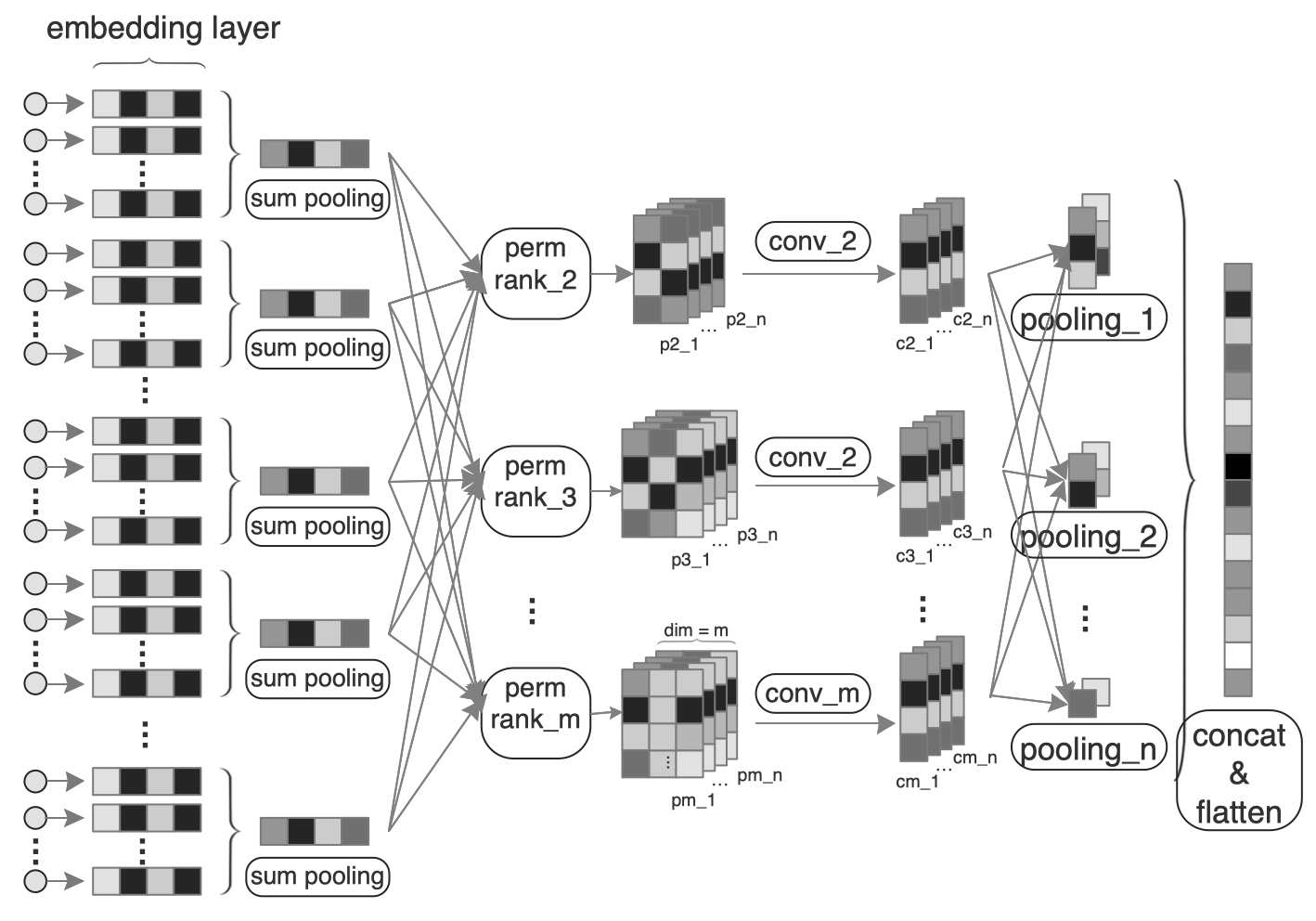
Figure 1: The structure of SSM we proposed. It introduces kinds of convolution and pooling operators on embedding vectors, which are able to find structured relations between features.

Among all those features of Table1, the user behavior and ad/item features are used for CTR prediction. It is difficult to figure out the representations of high level implicit features in feature engineering. Hence, it is critical to improve the performance of CTR by figuring out a good representation of high level implicit features.

DSSMHuang et al. (2013) was presented to find the semantic relation between query and doc. Based on DSSM, we introduce an structured convolution pooling network to find the structured semantic relation between high level implicit features. The dot-product of two embedding vectors, which is treated as a special convolution and pooling operators as Eq(3), are commonly used to represent the similarity of two ads/items.

$$pooling(Conv({e}_{1},{e}_{2}))={e}_{1}^{T}{e}_{2}$$ (3)

Therefore, we introduce a convolution and pooling layer to figure out the relations between embedding vectors, and optimize the cross-entropy loss with the predicted value ${\widehat{y}}$, and ${\widehat{y}}$ is sigmoid of trainable variables ${W}$ and input vector ${U}$.

Why convolution and pooling DNN can learn structured semantic relations from the user and item features? Our structured semantic model mainly contains three aspects:

• i) We introduce an embedding permutation of user and ad/item embedding vectors as Eq(4) and $m$ is the rank of permutation to characterize the number of features which interact with each other.

  $$C{{}_{n}^{m}}=\frac{{n}!}{{m}!({n-m}!)}$$ (4)

  The space complexity grows exponentially with the rank of feature permutation. Generally speaking, it is cost prohibitive when the rank is greater than 5. We permutate user-item combinations instead of all permutations to avoid this problem. The rank less than 4 could get good enough result. The number of permutation of features is showed in Eq(6), ${n_{1}}$ denotes the number of user features and ${n_{2}}$ denotes the number of ad/item features. We defined ${R}$ as a function of ${n_{1}}$ and ${n_{2}}$ to produce the combination of feature number, and defined ${P}$ as a cumulative of ${R}$.

  $${R}_{n1,n2}^{m}=\sum_{j=1}^{m-1}{C}_{n1}^{j}{C}_{n2}^{m-j}\ \ \ m=2,3,\ldots n$$ (5)

  $${P}_{n1,n2}^{r}=\sum_{i=2}^{r}{R}_{n1,n2}^{i}\ \ \ r=2,3,\ldots n$$ (6)

• ii) 1-d convolution is defined as Eq(7), ${e}$ denotes the embedding vector and ${K}$ denotes a convolution kernel. We adapt many kinds of 1-d linear convolution operators to describe how embedding vectors interact with each other and treat dot-product as a special convolution operator as same as other linear kernel functions(ie. [-1,1], [1,1]). Normally, the size of convolution kernel is set from [1,2] to [1,4] coresponding to the rank of permutation.

  $${Conv\_1d}([{k}_{1},{k}_{2}],{e}_{1},{e}_{2})={k}_{1}{e}_{1}+{k}_{2}{e}_{2}$$ (7)

  The 1-d convolution kernel shown in 8 was used in our practice (permutation rank 3 was used), which describes 5 linear and 1 special convolution kernels, and they are all orthogonal to each other. In addition, traditional CNN-based models train multi trainable convolution kernels(like [$w_{1}$,$w_{2}$]) also could get good enough result by lots of training epochs, but fixed orthogonal linear convolution kernels followed by a hidden layer could have much better performance, and we will explain it in later chapters.

  $$\begin{bmatrix}{dot\ product}\end{bmatrix}\quad\begin{bmatrix}1&-1\\ 1&1\end{bmatrix}\quad\begin{bmatrix}-1&1&1\\ 1&-1&1\\ 1&1&-1\end{bmatrix}\quad$$ (8)

  CNN-MSSChan et al. (2018) pointed out that using convolutional networks with multiple feature sequences could produce much more non-linear and deep representations, but training variables also get multiplied by the number of sequences which may not converge or could fall into local optimum easily. As show in our practice, use SSM instead of CNN-MSS could converge into better results.

• iii) We introduce a multi-scale pooling layer to figure out the relations between vectors. Pooling operations behind embedding vectors, can be viewed as a scale function similar to pooling in image and voice fields. Finally, we apply the logistic function McMahan et al. (2013) to the concat and flatten layer, and we name the last flatten layer of SSM multi-scale basic semantic representation of user and ad/item features.

Put It All Together

the flatten layer of SSM can be denoted as:

$${P} =Perm({r},\langle Emb({\theta_{1}},f_{1}),\ Emb({\theta_{2}},f_{2}),\ldots,\ Emb({\theta_{n}},f_{n})\rangle)$$ (9)

$${U} =Flatten(Pooling({s},Conv({k},{P}))$$ (10)

As shown in Eq(9), ${\theta_{1}}$ and ${\theta_{2}}$ denote the embedding matrix of user and item feature, $f_{1}$/$f_{2}$ denotes the input features, and ${r}$ is the rank of permutation which corresponds to the shape of convolution kernel ${k}$. The convolution kernels are matrices8, ${s}$ is the parameter of pooling operator(3,11 and 19 was set in our practice).

In our practice, firstly, we embed 3 user features and 2 item/ad features with the shape of embedding vector ${e}$ set to $[5K,100]$ and 20 sequences with shape $[100,2]$ and $[100,3]$ generated by a permutation of rank 2 and 3. Secondly, convolute these 20 sequences with 6 kernels whose shapes are $[1,2]$ and $[1,3]$ to generate 70 vectors . Thirdly, take pooling operation over 80 vectors with 3 kinds of pooling operators with window size set to 3, 7 and 13 to get 3 matrices ${p1_{[98,70]}}$, ${p2_{[32,70]}}$ and ${p3_{[15,70]}}$. Lastly, flatten the 3 pooling matrices ${p1,p2,p3}$ to a flattened vector ${Flt_{[1,10150]}}$ as the input of LR.

With the approach metioned above, the SSM learns feature embeddings and its multi-scale basic semantic representation for DNN which improves AUC of CTR prediction a lot. The embedding learned by SSM can describe the semantic information over features efficiently.

3.4 Multi-Scale Base Semantic Representation

We named the last flatten layer of SSM as Multi-Scale Base Semantic Representation, which together with the embedding vectors are fed into DNN as inputs.

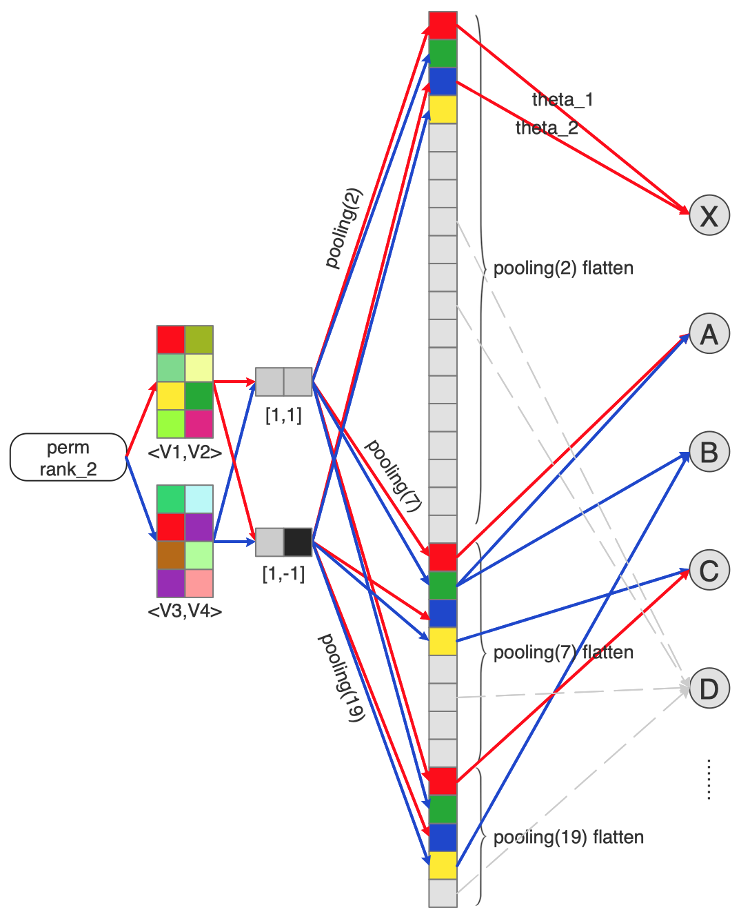
Figure 2: Multi-Scale Base Semantic Representation with hidden layer. The multi-scale base semantic representation followed by a hidden layer constructs non-linear relations between embedding vectors. The node ’X’ illustrates a convolution kernel $[\theta_{1}+\theta_{2},\theta_{1}-\theta_{2}]$ over $[V_{1},V_{2}]$, node ’B’ illustrates the relations between $[V_{3},V_{4}]$ in different scales. All nodes are fully connected with multi-scale base semantic representation just like node ’D’.

Base Semantic For signal processing, wavelet and fourier transformation play a critical role to transform signal from time domain to frequency domain. The base functions of wavelet are sine and cosine function. We propose the base function to CTR prediction, which contains two types of linear convolution kernels with shapes of $[1,2]$ and $[1,3]$, and a special convolution kernel with dot-product. In CNN-MSSChan et al. (2018) and other convolution related approaches, the convolution kernels are usually trainable, and a large number of feature mapping in CNN might results in overfitting and computational consumption. On the contrary, our base-formed kernels(8) are fixed and not trainable. Linear relations are represented by using properties of base functions and non-linear relations are represented by a hidden layer.

Multi-Scale. The multi-scale can be demonstrated by multiple pooling operators with various size.

In traditional CNN-based models, the convolution and pooling operators are independent. Pooling operator always follows convolution operators which means training process first determines the function, and then determines what kind of scale to put it on.

Aside from base functions mentioned above, there also exist lots of interactions among different pooling segments within the multi-scale embedding vector, such as interactions between word and word vectors, word and classification vectors, classification and classification vectors. We define it as multi-scale interaction modeling problem.

That process produces $Num(conv)*Num(pooling)$ parameters to train. For NLP and CTR prediction, interaction affections exist between multi-scale embeddings and the number of parameters of traditional CNN-based models will be too huge to get a good result.

Delay Convolution. The SSM we proposed in this paper can solve the problems efficiently. First of all, we produce series of base semantic representation using base functions (the matrices8 mentioned above), and then use hidden layer to choose convolution kernel types and pooling scale at the same time, which is named is delay convolution.

Node of hidden layer can be defined as Eq(11). SSM followed by a hidden layer gets better performance than traditional CNN-based models. Training convolution kernels and scale together reduces computation load and improves convergence speed. Additionally, the nodes of hidden layer in Fig2 can not only describe combinations across different base functions but also different scales which brings more non-linear relations. For instance, the relations between words and classifications can be expressed as a linear combination of two pooling operators with different scales.

$${N_{k}}=Relu\left(\sum_{i=0}^{N}\theta_{i}Pooling({S},Conv({K},{P}))\right)$$ (11)

3.5 SSM supported Wide&Deep

The multi-scale base semantic representation learned by SSM associates with inputs in DNN by simply concated to the flatten embeddings. In Eq(12), ${\widehat{y}}$ denotes the prediction value of CTR which is the output of sigmoid function $\sigma$ and $W_{wide}$ denotes the weights of origin features $X$ and feature engineering features $\phi(X)$, $W_{deep}$ denotes the weights of the output of DNN, and the red arrowhead denotes the multi-scale base semantic representation concat to the input of DNN. In Eq(13), $a^{(l_{0})}$ denotes the input of DNN which is a concatation of embeddings ${e_{i}}$ and the last layer of SSM ${U}$, and then $a^{(l_{0})}$ follows a standard MLP transform in Eq(1). The whole architecture of Wide&Deep-SSM show as Fig3.

$${\widehat{y}}=\sigma\left(W_{wide}^{T}{[X,\phi(X)]+W_{deep}^{T}{a^{(l_{f})}}}\right)$$ (12)

$${a^{l_{0}}}=concat\_flatten\left({e}_{1},{e}_{2},\ldots,{e}_{n},{U}\right)$$ (13)

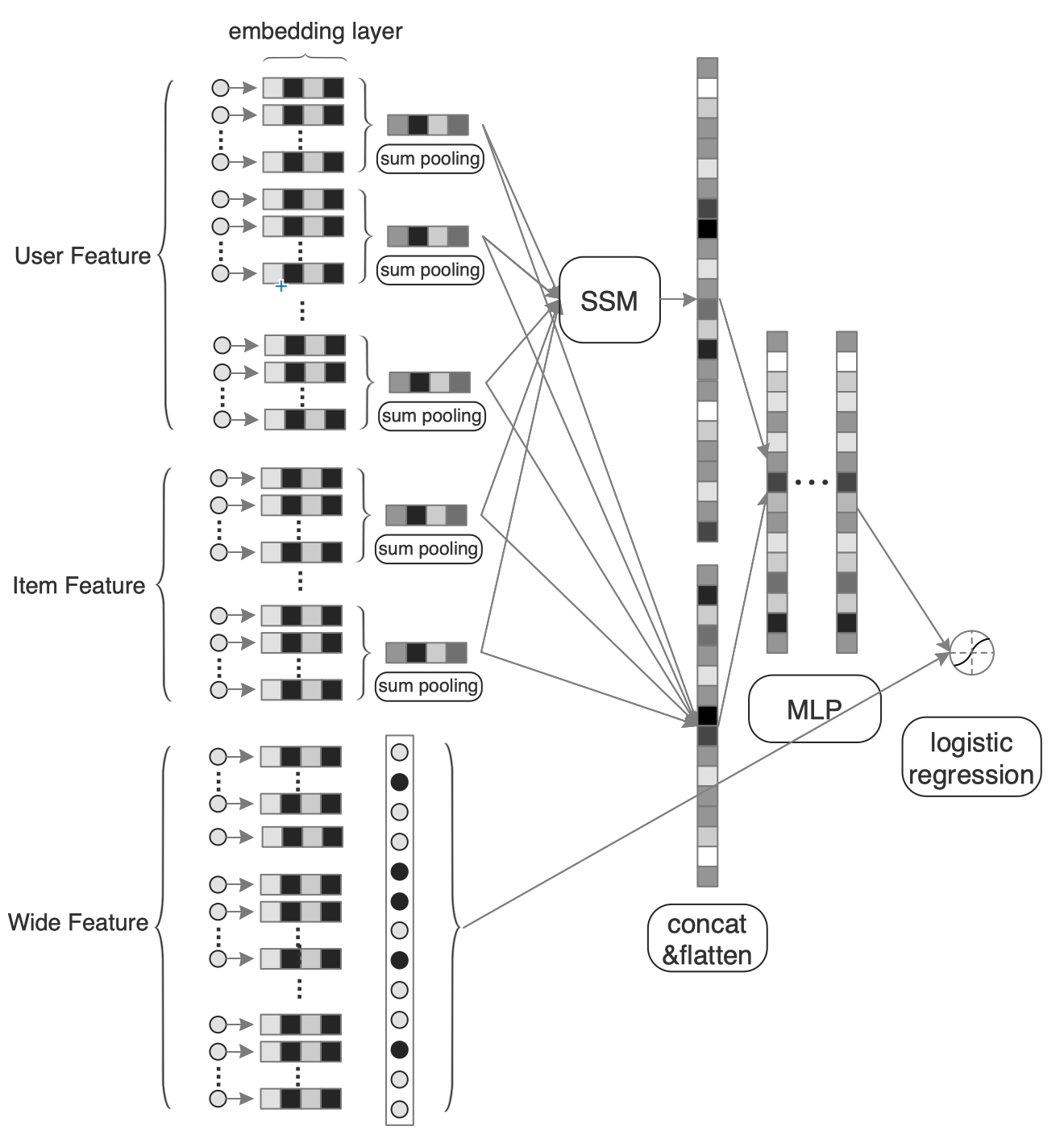
Figure 3: SSM supported Wide&Deep Architecture. Above show the structure of SSM supported Wide&Deep we proposed, it concat the output of SSM as partial input of DNN as same as the embeddings.

4 Experiments

In this section, our experiments are discussed in detail including the datasets, experimental settings, model comparisons and the corresponding analysis.

Both the public datasets and experiment codes are made available on github¹.

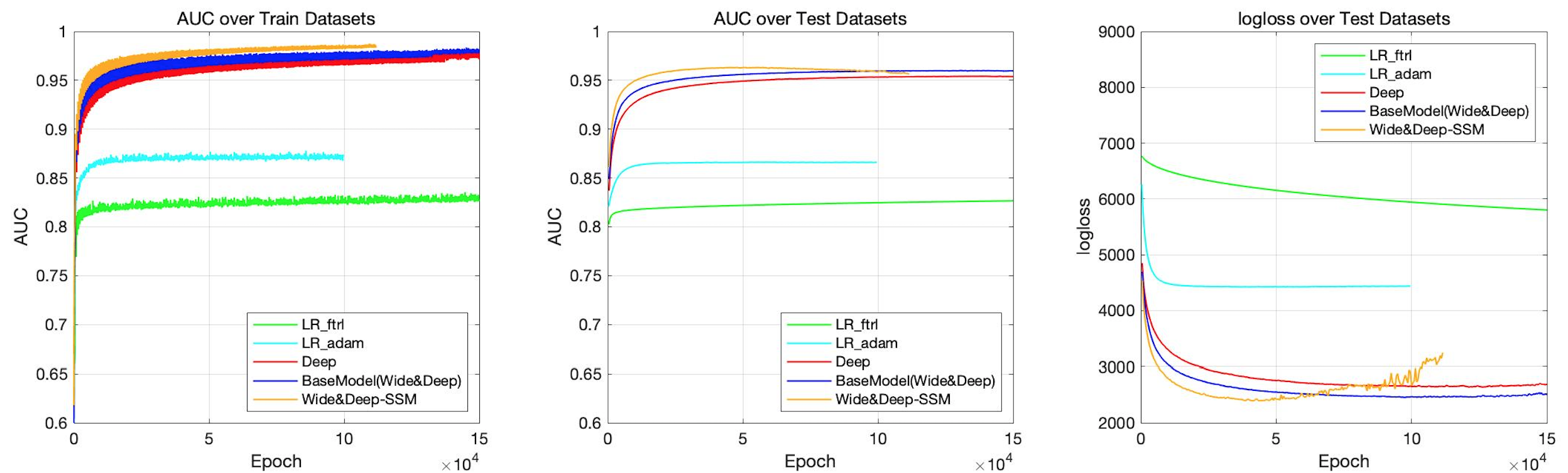
Figure 4: Performances of different model on Weibo Dataset. Wide&Deep-SSM shows the improvement over test logloss and AUC.

Table 2: Model Comparison on Avazu, MovieLens and Weibo Datasets. All the lines calculate RelaImpr by comparing with BaseModel on each dataset respectively.

Model	Avazu(Electro).		MovieLens.		Weibo.
	AUC	RelaImpr	AUC	RelaImpr	AUC	RelaImpr
LR	0.6525	-24.0%	0.6984	-25.2%	0.8371	-12.58%
Deep	0.6963	-2.19%	0.7576	-2.87%	0.8742	-2.98%
BaseModel(Wide&Deep)	0.7007	$\sim$	0.7652	$\sim$	0.8857	$\sim$
Wide&Deep-SSM	0.7011	0.2%	0.7754	3.9%	0.9109	6.55%

4.1 Datasets and Settings

We conduct experiments on Weibo dataset and two opensource datasets.

Avazu Dataset. In Avazu dataset, which is provided in 2014 Kaggle competition. The dataset contains 40 million samples with 22 fields for ten consecutive days, and all fields are used in our experiments. We use the samples of first nine days as training set and the samples of the tenth day for evaluation.

MovieLens Dataset. MovieLens dataHarper and Konstan (2015) contains 138,493 users, 27,278 movies, 21 categories and 20,000,263 samples. To make it suitable for CTR prediction task, we transform it into a binary classification data. Original user rating of the movies is continuous value ranging from 0 to 5. We label the samples as positive if the rating is above 3(e.g. 3.5,4.0,4.5,5.0), otherwise is negative.

Weibo Dataset. In Weibo dataset, we collected impression logs from the online display advertising system, of which two weeks’ samples are used for training and samples of the following day for testing. The size of training and testing set is about 1 billions and 0.1 billion respectively. 31 fields of features are separated into three categories (user profile, ad information and context information) for each sample.

4.2 Model Comparison

LR.McMahan et al. (2013) Logistic regression (LR) is a widely used in CTR prediction task because training is fast and results can be easily explained. We treate it as a weak baseline.

BaseModel(Wide&Deep Model).Cheng et al. (2016) The google’s wide&deep model has been widely used in real industrial applications. We treat it as the benchmark model. It consists of two parts: wide model, which handles the manually designed cross product features and deep model, which automatically extracts non-linear relations among features. We set it as BaseModel.

Wide&Deep-SSM. Defferent from Wide&Deep, the result of SSM concated to the input of DNN.

4.3 Performance of the Experiment

AUC is one of the most popular evaluation metrics for CTR prediction which measures the goodness of order by ranking all the ads with predicted CTR, including intra-user and inter-user orders. We adopt RelaImpr introduced in Yan et al. (2014) to measure relative improvement over models It is defined as follows:

$$RelaImpr=\left(\frac{\text{AUC(measured model)}-0.5}{\text{AUC(base model)}-0.5}-1\right)\times 100\%.$$ (14)

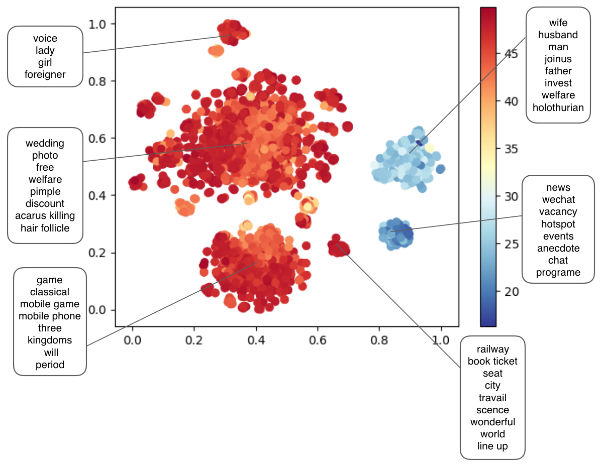
Figure 5: Visualization of flatten layer of samples in SSM. Shape of points represents a single sample. Color of points corresponds to CTR prediction value.

Fig4 shows the training and testing AUC on LR, base model and Wide&Deep-SSM. The statistics of all the above datasets is shown in Table2.

From Table2, we can see that, in terms of RelaImpr, all deep networks perform significantly better than LR, and Wide&Deep-SSM has the best performance.

4.4 Visualization of SSM

We take samples of different tags to visualize the learned multi-scale base semantic representation by two-dimensional scatter plot using t-SNEvan der Maaten and Hinton (2008). The cluster points represent the same types of items/ad texts. That means words from similar item/ad are almost aggregated together, which demonstrates the aggregation ability of SSM flatten vector. Besides, it’s also a Heat Map that different intensity indicate the prediction values (high intensity reveals high click prediction). Fig5 shows the distribution of users’ inclination to click advertisements in semantic space. As we can see, SSM can express a preference distribution in semantic space efficiently.

5 Conclusions

In this paper, we focus on the task of CTR prediction in online advertising with rich structured data. The performance of the embeddings of those structured data learned by DNN-based model is a bottleneck for the performance of the CTR prediction. To improve the performance of the embeddings, a novel approach named SSM is designed to pre-train the embeddings by structured semantic model to get semantic relations between features, and fine tune it with DNN variables. Additionally, we introduce series base convolution instead kinds of trainable convolutions to learn the multi-scale base semantic representation, and follow a hidden layer for complex interactions which we called delay convolution. SSM get good performance both in opensource dataset or Weibo dataset, and can be extend to other DNN-based models easily.

References

- [1]
- Bengio et al. [2003] Yoshua Bengio, Réjean Ducharme, Pascal Vincent, and Christian Jauvin. 2003. A neural probabilistic language model. JMLR (2003), 1137–1155.
- Chan et al. [2018] Patrick P. K. Chan, Xian Hu, Lili Zhao, Daniel S. Yeung, Dapeng Liu, and Lei Xiao. 2018. Convolutional Neural Networks based Click-Through Rate Prediction with Multiple Feature Sequences.. In IJCAI, Jérôme Lang (Ed.). ijcai.org, 2007–2013. http://dblp.uni-trier.de/db/conf/ijcai/ijcai2018.html#ChanHZYLX18
- Cheng et al. [2016] Heng-Tze Cheng, Levent Koc, Jeremiah Harmsen, Tal Shaked, Tushar Chandra, Hrishi Aradhye, Glen Anderson, Greg Corrado, Wei Chai, Mustafa Ispir, Rohan Anil, Zakaria Haque, Lichan Hong, Vihan Jain, Xiaobing Liu, and Hemal Shah. 2016. Wide & Deep Learning for Recommender Systems. CoRR abs/1606.07792 (2016). http://dblp.uni-trier.de/db/journals/corr/corr1606.html#ChengKHSCAACCIA16
- Covington et al. [2016] Paul Covington, Jay Adams, and Emre Sargin. 2016. Deep Neural Networks for YouTube Recommendations.. In RecSys, Shilad Sen, Werner Geyer, Jill Freyne, and Pablo Castells (Eds.). ACM, 191–198. http://dblp.uni-trier.de/db/conf/recsys/recsys2016.html#CovingtonAS16
- Gai et al. [2017] Kun Gai, Xiaoqiang Zhu, Han Li, Kai Liu, and Zhe Wang. 2017. Learning Piece-wise Linear Models from Large Scale Data for Ad Click Prediction. CoRR abs/1704.05194 (2017). http://dblp.uni-trier.de/db/journals/corr/corr1704.html#GaiZLLW17
- Guo et al. [2017] Huifeng Guo, Ruiming Tang, Yunming Ye, Zhenguo Li, and Xiuqiang He. 2017. DeepFM: A Factorization-Machine based Neural Network for CTR Prediction. CoRR abs/1703.04247 (2017). http://dblp.uni-trier.de/db/journals/corr/corr1703.html#GuoTYLH17
- Harper and Konstan [2015] F. Maxwell Harper and Joseph A. Konstan. 2015. The MovieLens Datasets: History and Context. ACM Trans. Interact. Intell. Syst. 5, 4, Article 19 (Dec. 2015), 19 pages. https://doi.org/10.1145/2827872
- Huang et al. [2013] Po-Sen Huang, Xiaodong He, Jianfeng Gao, Li Deng, Alex Acero, and Larry Heck. 2013. Learning Deep Structured Semantic Models for Web Search using Clickthrough Data. ACM International Conference on Information and Knowledge Management (CIKM). https://www.microsoft.com/en-us/research/publication/learning-deep-structured-semantic-models-for-web-search-using-clickthrough-data/
- McMahan et al. [2013] H. Brendan McMahan, Gary Holt, D. Sculley, Michael Young, Dietmar Ebner, Julian Grady, Lan Nie, Todd Phillips, Eugene Davydov, Daniel Golovin, Sharat Chikkerur, Dan Liu, Martin Wattenberg, Arnar Mar Hrafnkelsson, Tom Boulos, and Jeremy Kubica. 2013. Ad Click Prediction: A View from the Trenches. In Proceedings of the 19th ACM SIGKDD International Conference on Knowledge Discovery and Data Mining (KDD ’13). ACM, New York, NY, USA, 1222–1230. https://doi.org/10.1145/2487575.2488200
- Mikolov et al. [2011] Tomas Mikolov, Stefan Kombrink, Anoop Deoras, Lukas Burget, and Jan Honza Cernocky. 2011. RNNLM - Recurrent Neural Network Language Modeling Toolkit. https://www.microsoft.com/en-us/research/publication/rnnlm-recurrent-neural-network-language-modeling-toolkit/
- Qu et al. [2016] Yanru Qu, Han Cai, Kan Ren, Weinan Zhang, Yong Yu, Ying Wen, and Jun Wang. 2016. Product-based Neural Networks for User Response Prediction. CoRR abs/1611.00144 (2016). http://dblp.uni-trier.de/db/journals/corr/corr1611.html#QuCRZYWW16
- Rendle [2010] Steffen Rendle. 2010. Factorization Machines. In Proceedings of the 10th IEEE International Conference on Data Mining. IEEE Computer Society.
- Shan et al. [2016] Ying Shan, T. Ryan Hoens, Jian Jiao, Haijing Wang, Dong Yu, and J. C. Mao. 2016. Deep Crossing: Web-Scale Modeling without Manually Crafted Combinatorial Features.. In KDD, Balaji Krishnapuram, Mohak Shah, Alexander J. Smola, Charu C. Aggarwal, Dou Shen, and Rajeev Rastogi (Eds.). ACM, 255–262. http://dblp.uni-trier.de/db/conf/kdd/kdd2016.html#ShanHJWYM16
- van der Maaten and Hinton [2008] Laurens van der Maaten and Geoffrey Hinton. 2008. Visualizing Data using t-SNE. Journal of Machine Learning Research 9 (2008), 2579–2605. http://www.jmlr.org/papers/v9/vandermaaten08a.html
- Yan et al. [2014] Ling Yan, Wu-Jun Li, Gui-Rong Xue, and Dingyi Han. 2014. Coupled Group Lasso for Web-Scale CTR Prediction in Display Advertising.. In ICML (JMLR Workshop and Conference Proceedings), Vol. 32. JMLR.org, 802–810. http://dblp.uni-trier.de/db/conf/icml/icml2014.html#YanLXH14
- Zhang et al. [2016] Weinan Zhang, Tianming Du, and Jun Wang. 2016. Deep Learning over Multi-field Categorical Data - - A Case Study on User Response Prediction.. In ECIR (Lecture Notes in Computer Science), Nicola Ferro, Fabio Crestani, Marie-Francine Moens, Josiane Mothe, Fabrizio Silvestri, Giorgio Maria Di Nunzio, Claudia Hauff, and Gianmaria Silvello (Eds.), Vol. 9626. Springer, 45–57. http://dblp.uni-trier.de/db/conf/ecir/ecir2016.html#ZhangDW16
- Zhou et al. [2018] Guorui Zhou, Xiaoqiang Zhu, Chengru Song, Ying Fan, Han Zhu, Xiao Ma, Yanghui Yan, Junqi Jin, Han Li, and Kun Gai. 2018. Deep Interest Network for Click-Through Rate Prediction.. In KDD, Yike Guo and Faisal Farooq (Eds.). ACM, 1059–1068. http://dblp.uni-trier.de/db/conf/kdd/kdd2018.html#ZhouZSFZMYJLG18