Well-balanced finite volume schemes for hydrodynamic equations with general free energy

Abstract.

Well-balanced and free energy dissipative first- and second-order accurate finite volume schemes are proposed for a general class of hydrodynamic systems with linear and nonlinear damping. The variation of the natural Liapunov functional of the system, given by its free energy, allows, for a characterization of the stationary states by its variation. An analog property at the discrete level enables us to preserve stationary states at machine precision while keeping the dissipation of the discrete free energy. These schemes can accurately analyse the stability properties of stationary states in challenging problems such as: phase transitions in collective behavior, generalized Euler-Poisson systems in chemotaxis and astrophysics, and models in dynamic density functional theories; having done a careful validation in a battery of relevant test cases.

1. Introduction

The construction of robust well-balanced numerical methods for conservation laws has attracted a lot of attention since the initial works of LeRoux and collaborators [40, 38]. The well-balanced property is equivalent to the exact C-property defined beforehand by Bermúdez and Vázquez in [5], and both of them refer to the ability of a numerical scheme to preserve the steady states at a discrete level and to accurately compute evolutions of small deviations from them. The historical evolution of well-balanced schemes is reviewed in [37]. On the other hand, the derivation of numerical schemes preserving structural properties of the evolutions under study such as dissipations or conservations of relevant physical quantities is an important line of research in hydrodynamic systems and their overdamped limits, see for instance [23, 10, 68, 60]. In the present work, we propose numerical schemes with well-balanced and free energy dissipation properties for a general class of balance laws or hydrodynamic models with attractive-repulsive interaction forces, and linear or nonlinear damping effects, such as the Cucker-Smale alignment term in swarming. The general hydrodynamic system has the form

(1) $$\begin{cases}\partial_{t}\rho+\nabla\cdot\left(\rho\bm{u}\right)=0,\quad\bm{x}\in\mathbb{R}^{d},\quad t>0,\\[5.69054pt] {\displaystyle\partial_{t}(\rho\bm{u})\!+\!\nabla\!\cdot\!(\rho\bm{u}\otimes\bm{u})\!=-\nabla P(\rho)-\rho\nabla H(\bm{x},\rho)-\gamma\rho\bm{u}-\!\rho\!\!\!\int_{\mathbb{R}^{d}}\!\!\psi(\bm{x}-\bm{y})(\bm{u}(\bm{x})-\bm{u}(\bm{y}))\rho(\bm{y})\,d\bm{y},}\end{cases}$$

where $\rho=\rho(\bm{x},t)$ and $\bm{u}=\bm{u}(\bm{x},t)$ are the density and the velocity, $P(\rho)$ is the pressure, $H(\bm{x},\rho)$ contains the attractive-repulsive effects from external $V$ or interaction potentials $W$, assumed to be locally integrable, given by

$$H(\bm{x},\rho)=V(\bm{x})+W(\bm{x})\star\rho,$$

and $\psi(\bm{x})$ is a nonnegative symmetric smooth function called the communication function in the Cucker-Smale model [21, 22] describing collective behavior of systems due to alignment [11].

The fractional-step methods [52] have been the widely-employed tool to simulate the temporal evolution of balance laws such as (1). They are based on a division of the problem in (1) into two simpler subproblems: the homogeneous hyperbolic system without source terms and the temporal evolution of density and momentum without the flux terms but including the sources. These subproblems are then resolved alternatively employing suitable numerical methods for each. This procedure introduces a splitting error which is acceptable for the temporal evolution, but becomes critical when the objective is to preserve the steady states. This is due to the fact that the steady state is reached when the fluxes are exactly balanced with the source terms in each discrete node of the domain. However, when solving alternatively the two subproblems, this discrete balance can never be achieved, since the fluxes and source terms are not resolved simultaneously.

To correct this deficiency, well-balanced schemes are designed to discretely satisfy the balance between fluxes and sources when the steady state is reached [6]. The strategy to construct well-balanced schemes relies on the fact that, when the steady state is reached, there are some constant relations of the variables that hold in the domain. These relations allow the resolution of the fluxes and sources in the same level, thus avoiding the division that the fractional-step methods introduce. Moreover, if the system enjoys a dissipative property and it has a Liapunov functional, obtaining analogous tools at the discrete level is key for the derivation of well-balanced schemes. In this work the steady-state relations and the dissipative property are obtained by means of the associated free energy, which in the case of the system in (1) is formulated as

(2) $$\mathcal{F}[\rho]=\int_{\mathbb{R}^{d}}\Pi(\rho)d\bm{x}+\int_{\mathbb{R}^{d}}V(\bm{x})\rho(\bm{x})d\bm{x}+\frac{1}{2}\int_{\mathbb{R}^{d}}\int_{\mathbb{R}^{d}}W(\bm{x}-\bm{y})\rho(\bm{x})\rho(\bm{y})d\bm{x}d\bm{y},$$

where

(3) $$\rho\Pi^{\prime\prime}(\rho)=P^{\prime}(\rho).$$

The pressure $P(\rho)$ and the potential term $H(\bm{x},\rho)$ appearing in the general system (1) can be gathered by considering the associated free energy. Taking into account that the variation of the free energy in (2) with respect to the density $\rho$ is equal to

(4) $$\frac{\delta\mathcal{F}}{\delta\rho}=\Pi^{\prime}(\rho)+H(\bm{x},\rho),$$

it follows that the general system (1) can be written in a compact form as

(5) $$\begin{cases}\partial_{t}\rho+\nabla\cdot\left(\rho\bm{u}\right)=0,\quad\bm{x}\in\mathbb{R}^{d},\quad t>0,\\[5.69054pt] {\displaystyle\partial_{t}(\rho\bm{u})\!+\!\nabla\!\cdot\!(\rho\bm{u}\otimes\bm{u})\!=-\rho\nabla\frac{\delta\mathcal{F}}{\delta\rho}-\gamma\rho\bm{u}-\!\rho\!\!\int_{\mathbb{R}^{d}}\!\!\psi(\bm{x}-\bm{y})(\bm{u}(\bm{x})-\bm{u}(\bm{y}))\rho(\bm{y})\,d\bm{y}.}\end{cases}$$

The system in (5) is rather general containing a wide variety of physical problems all under the so-called density functional theory (DFT) and its dynamic extension (DDFT) see e.g. [32, 33, 34, 78, 79, 25] and the references therein. A variety of well-balanced schemes have already been constructed for specific choices of the terms $\Pi(\rho)$, $V(\bm{x})$ and $W(\bm{x})$ in the free energy (2), see [1, 6, 27] for instance. Here the focus is set on the free energy and the natural structure of the system (5). It is naturally advantageous to consider the concept of free energy in the construction procedure of well-balanced schemes, since they rely on relations that hold in the steady states, and moreover, the variation of the free energy with respect to the density is constant when reaching these steady states, more precisely

(6) $$\frac{\delta\mathcal{F}}{\delta\rho}=\Pi^{\prime}(\rho)+H(\bm{x},\rho)=\text{constant on each connected component of}\ \mathrm{supp}(\rho)\ \text{and}\ u=0,$$

where the constant can vary on different connected components of $\mathrm{supp}(\rho)$. As a result, the constant relations in the steady states, which are needed for well-balanced schemes, are directly provided by the variation of the free energy with respect to the density.

The steady state relations in (6) hold due to the dissipation of the linear damping $-\rho\bm{u}$ or nonlinear damping in the system (1), which eventually eliminates the momentum of the system. This can be justified by means of the total energy of the system, defined as the sum of kinetic and free energy,

(7) $$E(\rho,\bm{u})=\int_{\mathbb{R}^{d}}\frac{1}{2}\rho\left|\bm{u}\right|^{2}d\bm{x}+\mathcal{F}(\rho),$$

since it is formally dissipated, see [31, 15, 18], as

(8) $$\frac{dE(\rho,\bm{u})}{dt}=-\gamma\int_{\mathbb{R}^{d}}\rho\left|\bm{u}\right|^{2}d\bm{x}-\!\int_{\mathbb{R}^{d}}\int_{\mathbb{R}^{d}}\!\!\psi(\bm{x}-\bm{y})\left|\bm{u}(\bm{y})-\bm{u}(\bm{x})\right|^{2}\rho(\bm{x})\,\rho(\bm{y})\,d\bm{x}\,d\bm{y}.$$

This last dissipation equation ensures that the total energy $E(\rho,\bm{u})$ keeps decreasing in time while there is kinetic energy in the system. At the same time, since the definition of the total energy (7) also depends on the velocity $\bm{u}$, it results that the velocity throughout the domain eventually vanishes. When $\bm{u}=\bm{0}$ throughout the domain, the momentum equation in (5) reduces to

$$\rho\nabla\frac{\delta\mathcal{F}}{\delta\rho}=\bm{0},$$

meaning that in the support of the density the steady state relation (6) holds. However, for those points outside the support of the density and satisfying $\rho=0$, the variation of the free energy with respect to the density does not need to keep the constant value when the steady state is reached. A discussion of the resulting steady states depending on $\Pi(\rho)$ and $H(\bm{x},\rho)$ is provided in [10, 16, 41].

The system (1) also satisfies an entropy identity

(9) $$\partial_{t}\eta(\rho,\rho\textbf{u})+\nabla\cdot\bm{G}(\rho,\rho\textbf{u})=-\rho\bm{u}\cdot\nabla H(\bm{x},\rho)-\gamma\rho\left|\bm{u}\right|^{2}-\rho\int_{\mathbb{R}^{d}}\!\!\psi(\bm{x}-\bm{y})\,\bm{u}(\bm{x})\cdot(\bm{u}(\bm{x})-\bm{u}(\bm{y}))\rho(\bm{y})\,d\bm{y},$$

where $\eta(\rho,\rho\bm{u})$ and $\bm{G}(\rho,\rho\bm{u})$ are the entropy and the entropy flux defined as

(10) $$\eta(\rho,\rho\bm{u})=\rho\frac{\left|\bm{u}\right|^{2}}{2}+\Pi(\rho),\quad\bm{G}(\rho,\rho\bm{u})=\rho\bm{u}\left(\frac{\left|\bm{u}\right|^{2}}{2}+\Pi^{\prime}(\rho)\right).$$

From a physical point of view the entropy is always a convex function of the density [49]. As a result, from (10) it is justified to assume that $\Pi(\rho)$ is convex, meaning that $\Pi^{\prime}(\rho)$ has an inverse function for positive densities $\rho$. This last fact is a necessary requirement for the construction of the well-balanced schemes of this work, as it is explained in section 2. Finally, notice that from the entropy identity (9), one recovers the free energy dissipation (8) by integration using the continuity equation to deal with the forces term $H(\bm{x},\rho)$ and using symmetrization of the nonlinear damping term due to $\psi$ being symmetric.

Let us also point out that the evolution of the center of mass of the density can be computed in some particular cases. In fact, it is not difficult to deduce from (5) that

(11) $$\frac{d}{dt}\int_{\mathbb{R}^{d}}\bm{x}\rho d\bm{x}=\int_{\mathbb{R}^{d}}\rho\bm{u}d\bm{x}\quad\mbox{and}\quad\frac{d}{dt}\int_{\mathbb{R}^{d}}\rho\bm{u}d\bm{x}=-\int_{\mathbb{R}^{d}}\nabla V(\bm{x})\rho d\bm{x}-\gamma\int_{\mathbb{R}^{d}}\rho\bm{u}d\bm{x}\,,$$

due to the antisymmetry of $\nabla W(\bm{x})$ and the symmetry of $\psi(\bm{x})$. Therefore, in case $V(\bm{x})$ is not present or quadratic, (11) are explicitly solvable. Moreover, if the potential $V(\bm{x})$ is symmetric, the initial data for the density is symmetric, and the initial data for the velocity is antisymmetric, then the solution to (5) keeps these symmetries in time, i.e., the density is symmetric and the velocity is antisymetric for all times, and the center of mass is conserved

$$\frac{d}{dt}\int_{\mathbb{R}^{d}}\bm{x}\rho d\bm{x}=0\,.$$

The steady state relations (6) only hold when the linear damping term is included in system (1). When only the nonlinear damping of Cucker-Smale type is present, the system has the so-called moving steady states, see [13, 11, 18], which satisfy the more general relations

(12) $$\frac{\delta\mathcal{F}}{\delta\rho}=\text{constant on each connected component of}\ \mathrm{supp}(\rho)\ \text{and}\ \bm{u}=\text{constant}.$$

However, the construction of well-balanced schemes satisfying the moving steady state relations has proven to be more difficult than for the still steady states (6) without dissipation. For literature about well-balanced schemes for moving steady states without dissipation, we refer to [58, 76].

The most popular application in the literature for well-balanced schemes deals with the Saint-Venant system for shallow water flows with nonflat bottom [1, 6, 9, 53, 72, 75], for which $\Pi(\rho)=\frac{g}{2}\rho^{2}$, with $g$ being the gravity constant, and $H(\bm{x},\rho)$ depends on the bottom. Here it is important to remark the work of Audusse et al. in [1], where they propose a hydrostatic reconstruction that has successfully inspired more sophisticated well-balanced schemes in the area of shallow water equations [55, 57]. Another area where well-balanced schemes have been fruitful is chemosensitive movement, with the works of Filbet, Shu and their collaborators [26, 27, 36, 74]. In this case the pressure satisfies $\Pi(\rho)=\rho\left(\ln(\rho)-1\right)$ and $H$ depends on the chemotactic sensitivity and the chemical concentration. The list of applications of the system (1) continues growing with more choices of $\Pi(\rho)$ and $H(\bm{x},\rho)$ [74]: the elastic wave equation, nozzle flow problem, two phase flow model, etc.

The orders of accuracy from the finite volume well-balanced schemes presented before range from first- and second-order [1, 51, 77, 48, 53] to higher-order versions [74, 71, 57, 28]. Again, the most popular application has been shallow water equations, and the survey from Xing and Shu [75] provides a summary of all the shallow water methods with different accuracies. Some of the previous schemes proposed were equipped to satisfy natural properties of the systems under consideration, such as nonnegativity of the density [2, 48] or the satisfaction of a discrete entropy inequality [1, 27], enabling also the computation of dry states [28] . Theoretically the Godunov scheme satisfies all these properties [50], but its main drawback is its computationally expensive implementation. The high-order schemes usually rely on the WENO reconstructions originally proposed by Jiang and Shu [43].

Other well-balanced numerical approaches employed to simulate the system (5) are finite differences [73, 72], which are equivalent to the finite volume methods for first-and second-order, and the discontinuous Galerkin methods [74]. The overdamped system of (5) with $\psi\equiv 0$, obtained in the free inertia limit where the momentum reaches equilibrium on a much faster timescale than the density, has also been numerically resolved for general free energies of the form (2), via finite volume schemes [10] or discontinuous Galerkin approaches [68]. This scheme for the overdamped system also conserves the dissipation of the free energy at the discrete approximation.

The novelty of this work is twofold. Foremost, all these previous schemes were only applicable for specific choices of $\Pi(\rho)$ and $H(\bm{x},\rho)$, meaning that a general scheme valid for a wide range of applications is lacking. And while some previous schemes [74] could be employed in more general cases, the focus in the literature has been on the shallow water and chemotaxis equations. In addition, the function $H(\bm{x},\rho)$, which results from summing $V(\bm{x})$ and $W(\bm{x})\star\rho$ as in (1), has so far been taken as dependent on $\bm{x}$ only, unlike the present work where it depends on $\rho$ by means of the convolution with an interaction potential $W(\bm{x})$.

In this work we present a finite volume scheme for a general choice of $\Pi(\rho)$ and $H(\bm{x},\rho)$ which is first- and second-order accurate and satisfies the nonnegativity of the density, the well-balanced property, the semidiscrete entropy inequality and the semidiscrete free energy dissipation. Furthermore, as it is shown in example 3.9 of section 3, it can also be applied to more general free energies than the one in (2) and with the form

(13) $$\mathcal{F}[\rho]=\int_{\mathbb{R}^{d}}\Pi(\rho)d\bm{x}+\int_{\mathbb{R}^{d}}V(\bm{x})\rho(\bm{x})d\bm{x}+\frac{1}{2}\int_{\mathbb{R}^{d}}K\left(W(\bm{x})\star\rho(\bm{x})\right)\rho(\bm{x})d\bm{x},$$

where $K$ is a function depending on the convolution of $\rho(\bm{x})$ with the kernel $W(\bm{x})$. Its variation with respect to the density satisfies

(14) $$\frac{\delta\mathcal{F}}{\delta\rho}=\Pi^{\prime}(\rho)+V(\bm{x})+\frac{1}{2}K\left(W(\bm{x})\star\rho\right)+\frac{1}{2}K^{\prime}\left(W(\bm{x})\star\rho\right)\left(W(\bm{x})\star\rho\right).$$

These free energies arise in applications related to (D)DFT[25, 33], see [14] for other related free energies and properties.

The other novel technical aspect of this work concerns the numerical treatment of the different source terms in (1). In fact, in order to keep the well-balanced property and the decay of the free energy we treat source terms differently. While the dissipative terms are harmless and treated by direct approximations, the fundamental question is how to choose the discretization of the potential term given by $H(\bm{x},\rho)=V(\bm{x})+W(\bm{x})\star\rho$. For this purpose we appropriately extend the ideas in [6, 27] to our case to keep the well-balanced property and the energy decay. The condition for stationary states (6) is crucial in defining an approximation of the term $-\rho\nabla H(\bm{x},\rho)$ by a dicretization of $\nabla P(\rho)$ which is consistent when the new reconstructed values of the density at the interfaces taking into account the potential $H(\bm{x},\rho)$. This general treatment includes as specific cases both the shallow-water equations [1, 6] and the hyperbolic chemotaxis problem [27].

Section 2 describes the first- and second-order well-balanced scheme reconstructions, and provides the proofs of their main properties. Section 3 contains the numerical simulations, with a first subsection 3.1 where the validation of the well-balanced property and the orders of accuracy is conducted, and a second subsection 3.2 with numerical experiments from different applications. A wide range of free energies is employed to remark the extensive nature of our well-balanced scheme. A short summary and conclusions are offered in section 4.

2. Well-balanced finite volume scheme

The terms appearing in the one-dimensional system (5) are usually gathered in the form of

(15) $$\partial_{t}U+\partial_{x}F(U)=S(x,U),$$

with

$$U=\begin{pmatrix}\rho\\ \rho u\end{pmatrix},\quad F(U)=\begin{pmatrix}\rho u\\ \rho u^{2}+P(\rho)\end{pmatrix}$$

and

$$S(x,U)=\begin{pmatrix}0\\ -\rho\partial_{x}H-\gamma\rho u-\rho\displaystyle\int_{\mathbb{R}}\psi(x-y)(u(x)-u(y))\rho(y)\,dy\end{pmatrix},$$

where $U$ are the unknown variables, $F(U)$ the fluxes and $S(U)$ the sources. The one-dimensional finite volume approximation of (15) is obtained by breaking the domain into grid cells $\left(x_{i-1/2}\right)_{i\in\mathbb{Z}}$ and approximating in each of them the cell average of $U$. Then these cell averages are modified after each time step, depending on the flux through the edges of the grid cells and the cell average of the source term [52]. Finite volume schemes for hyperbolic systems employ an upwinding of the fluxes and in the semidiscrete case they provide a discrete version of (15) under the form

(16) $$\dfrac{dU_{i}}{dt}=-\dfrac{F_{i+\frac{1}{2}}-F_{i-\frac{1}{2}}}{\Delta x_{i}}+S_{i},$$

where the cell average of $U$ in the cell $\left(x_{i-\frac{1}{2}},x_{i+\frac{1}{2}}\right)$ is denoted as

$$U_{i}=\begin{pmatrix}\rho_{i}\\ \rho_{i}u_{i}\end{pmatrix},$$

$F_{i+\frac{1}{2}}$ is an approximation of the flux $F(U)$ at the point $x_{i+\frac{1}{2}}$, $S_{i}$ is an approximation of the source term $S(x,U)$ in the cell $\left(x_{i-\frac{1}{2}},x_{i+\frac{1}{2}}\right)$ and $\Delta x_{i}$ is the possibly variable mesh size $\Delta x_{i}=x_{i+\frac{1}{2}}-x_{i-\frac{1}{2}}$.

The approximation of the flux $F(U)$ at the point $x_{i+\frac{1}{2}}$, denoted as $F_{i+\frac{1}{2}}$, is achieved by means of a numerical flux $\mathscr{F}$ which depends on two reconstructed values of $U$ at the left and right of the boundary between the cells $i$ and $i+1$. These two values, $U_{i+\frac{1}{2}}^{-}$ and $U_{i+\frac{1}{2}}^{+}$, are computed from the cell averages following different construction procedures that seek to satisfy certain properties, such as order of accuracy or nonnegativity. Two widely-employed reconstruction procedures are the second-order finite volume monotone upstream-centered scheme for conservation laws, referred to as MUSCL [59], or the weighted-essentially non-oscllatory schemes, widely known as WENO [66].

Once these two reconstructed values are computed, $F_{i+\frac{1}{2}}$ is obtained from

(17) $$F_{i+\frac{1}{2}}=\mathscr{F}\left(U_{i+\frac{1}{2}}^{-},U_{i+\frac{1}{2}}^{+}\right).$$

The numerical flux $\mathscr{F}$ is usually denoted as Riemann solver, since it provides a stable resolution of the Riemann problem located at the cell interfaces, where the left value of the variables in $U_{i+\frac{1}{2}}^{-}$ and the right value $U_{i+\frac{1}{2}}^{+}$. The literature concerning Riemann solvers is vast and there are different choices for it [69]: Godunov, Lax-Friedrich, kinetic, Roe, etc. Some usual properties of the numerical flux that are assumed [1, 6, 27] are:

1. It is consistent with the physical flux, so that $\mathscr{F}(U,U)=F(U)$.

2. It preserves the nonnegativity of the density $\rho_{i}(t)$ for the homogeneous problem, where the numerical flux is computed as in (17).

3. It satisfies a cell entropy inequality for the entropy pair (10) for the homogeneous problem. Then, according to [6], it is possible to find a numerical entropy flux $\mathscr{G}$ such that

   (18) $$\hskip 25.6073ptG(U_{i+1})+\nabla_{U}\,\eta(U_{i+1})\left(\mathscr{F}(U_{i},U_{i+1})-F(U_{i+1})\right)\\ \leq\mathscr{G}(U_{i},U_{i+1})\leq G(U_{i})+\nabla_{U}\,\eta(U_{i})\left(\mathscr{F}(U_{i},U_{i+1})-F(U_{i})\right),$$

   where $\nabla_{U}\,\eta$ is the derivative of $\eta$ with respect to $U=\begin{pmatrix}\rho\\ \rho u\end{pmatrix}$.

The first- and second-order well-balanced schemes described in this section propose an alternative reconstruction procedure for $U_{i+\frac{1}{2}}^{-}$ and $U_{i+\frac{1}{2}}^{+}$ which ensures that the steady state in (6) is discretely preserved when starting from that steady state. Subsections 2.1 and 2.3 contain the first- and second-order schemes, respectively, together with their proved properties.

2.1. First-order scheme

The basic first-order schemes approximate the flux $F_{i+\frac{1}{2}}$ by a numerical flux $\mathscr{F}$ which depends on the cell averaged values of $U$ at the two adjacent cells, so that the inputs for the numerical flux in (17) are

(19) $$F_{i+\frac{1}{2}}=\mathscr{F}\left(U_{i},U_{i+1}\right).$$

The resolution of the finite volume scheme in (16) with a numerical flux of the form in (19) and a cell-centred evaluation of $-\rho\partial_{x}H$ for the source term $S_{i}$ is not generally able to preserve the steady states, as it was shown in the initial works of well-balanced schemes [40, 38]. These steady states are provided in (6), and satisfy that the variation of the free energy with respect to the density has to be constant in each connected component of the support of the density. The discrete steady state is defined in a similar way,

(20) $$\left(\frac{\delta\mathcal{F}}{\delta\rho}\right)_{i}=\Pi^{\prime}(\rho_{i})+H_{i}=C_{\Gamma}\text{ in each}\ \Lambda_{\Gamma},\Gamma\in\mathbb{N}\,,$$

where $\Lambda_{\Gamma}$, $\Gamma\in\mathbb{N}$, denotes the possible infinite sequence indexed by $\Gamma$ of subsets $\Lambda_{\Gamma}$ of subsequent indices $i\in\mathbb{Z}$ where $\rho_{i}>0$ and $u_{i}=0$, and $C_{\Gamma}$ the corresponding constant in that connected component of the discrete support.

As it was emphasized above, the preservation of these steady states for particular choices of $\Pi^{\prime}(\rho)$ and $H(x,\rho)$, such as shallow water [1] or chemotaxis [27], is paramount. A solution to allow this preservation was proposed in the work of Audusse et al. [1], where instead of evaluating the numerical flux as in (17), they chose

(21) $$F_{i+\frac{1}{2}}=\mathscr{F}\left(U_{i+\frac{1}{2}}^{-},U_{i+\frac{1}{2}}^{+}\right),\ \text{where}\ U_{i+\frac{1}{2}}^{\pm}=\begin{pmatrix}\rho_{i+\frac{1}{2}}^{\pm}\\ \rho_{i+\frac{1}{2}}^{\pm}u_{i+\frac{1}{2}}^{\pm}\end{pmatrix}.$$

The interface values $U_{i+\frac{1}{2}}^{\pm}$ are reconstructed from $U_{i}$ and $U_{i+1}$ by taking into account the steady state relation in (20). Contrary to other works in which the interface values are reconstructed to increase the order of accuracy, now the objective is to satisfy the well-balanced property. Bearing this in mind, we make use of (20) to the cells with centred nodes at $x_{i}$ and $x_{i+1}$ to define the interface values such that

$$\begin{gathered}\Pi^{\prime}\left(\rho_{i+\frac{1}{2}}^{-}\right)+H_{i+\frac{1}{2}}=\Pi^{\prime}\left(\rho_{i}\right)+H_{i},\\ \Pi^{\prime}\left(\rho_{i+\frac{1}{2}}^{+}\right)+H_{i+\frac{1}{2}}=\Pi^{\prime}\left(\rho_{i+1}\right)+H_{i+1},\end{gathered}$$

where the term $H_{i+\frac{1}{2}}$ is evaluated to preserve consistency and stability, with an upwind or average value obtained as

(22) $$H_{i+\frac{1}{2}}=\max\left(H_{i},H_{i+1}\right)\quad\textrm{or}\quad H_{i+\frac{1}{2}}=\frac{1}{2}\left(H_{i}+H_{i+1}\right).$$

Then, by denoting as $\xi(s)$ the inverse function of $\Pi^{\prime}(s)$ for $s>0$, we conclude that the interface values $U_{i+\frac{1}{2}}^{\pm}$ are computed as

(23) $$\begin{gathered}\rho_{i+\frac{1}{2}}^{-}=\xi\left(\Pi^{\prime}\left(\rho_{i}\right)+H_{i}-H_{i+\frac{1}{2}}\right)_{+},\quad u_{i+\frac{1}{2}}^{-}=u_{i},\\ \rho_{i+\frac{1}{2}}^{+}=\xi\left(\Pi^{\prime}\left(\rho_{i+1}\right)+H_{i+1}-H_{i+\frac{1}{2}}\right)_{+},\quad u_{i+\frac{1}{2}}^{+}=u_{i+1}.\end{gathered}$$

The function $\xi(s)$ is well-defined for $s>0$ since $\Pi(s)$ is strictly convex, $\Pi^{\prime\prime}(s)>0$. This is always the case since, as mentioned in the introduction, the physical entropies are always strictly convex from (10). However, some physical entropies and applications allow for vacuum of the steady states, therefore we need to impose the value of $\rho_{i+\frac{1}{2}}^{\pm}$, given that they should be nonnegative. Henceforth, $\xi(s)$ denotes the extension by zero of the inverse of $\Pi^{\prime}(s)$ whenever $s>0$.

Furthermore, the discretization of the source term is taken as

(24) $$S_{i}=\frac{1}{\Delta x_{i}}\begin{pmatrix}0\\ P\left(\rho_{i+\frac{1}{2}}^{-}\right)-P\left(\rho_{i-\frac{1}{2}}^{+}\right)\end{pmatrix}-\begin{pmatrix}0\\ \gamma\rho_{i}u_{i}+\rho_{i}\displaystyle\sum_{j}\Delta x_{j}(u_{i}-u_{j})\rho_{j}\psi_{ij}\end{pmatrix},$$

which is motivated by the fact that in the steady state, with $u=0$ in (15), the fluxes are balanced with the sources,

$$\rho\partial_{x}\Pi^{\prime}(\rho)=-\rho\partial_{x}H.$$

Here, $\psi_{ij}$ is an approximation of the average value of $\psi$ on the interval centred at $x_{i}-x_{j}$ of length $\Delta x_{j}$. From here, and integrating over the cell volume, it results that

(25) $$\int_{x_{i-\frac{1}{2}}}^{x_{i+\frac{1}{2}}}-\rho\partial_{x}H\,dx=\int_{x_{i-\frac{1}{2}}}^{x_{i+\frac{1}{2}}}\rho\partial_{x}\Pi^{\prime}(\rho)\,dx=\int_{x_{i-\frac{1}{2}}}^{x_{i+\frac{1}{2}}}\partial_{x}P(\rho)\,dx=P(\rho_{i+\frac{1}{2}}^{-})-P(\rho_{i-\frac{1}{2}}^{+}),$$

with the relation between $\Pi^{\prime}(\rho)$ and $P(\rho)$ was given in (3). This idea of distributing the source terms along the interfaces has already been explored in previous works [44].

The discretization of the source term in (24) entails that the discrete balance between fluxes and sources is accomplished when $F_{i+\frac{1}{2}}=P(\rho_{i+\frac{1}{2}}^{-})=P(\rho_{i+\frac{1}{2}}^{+})$. The computation of the numerical fluxes expressed in (21), in which the interface values $U_{i+\frac{1}{2}}^{\pm}$ are considered, enables this balance if in the steady states $U_{i+\frac{1}{2}}^{-}=U_{i+\frac{1}{2}}^{+}=(\rho_{i+\frac{1}{2}}^{-},0)=(\rho_{i+\frac{1}{2}}^{+},0)$. Moreover, the discretization of the source term as in (24) may seem counter-intuitive when the system is far away from the steady state, given that the balanced expressed in (25) only holds in those states. In spite of this, the consistency with the original system in (15) is not lost, as it will be proved in subsection 2.2.

Let us finally discuss the discretization of the potential $H(x,\rho)=V(x)+W\ast\rho(x)$. We will always approximate it as

$$H_{i}=V_{i}+\sum_{j}\Delta x_{j}W_{ij}\rho_{j}\,,\mbox{ for all }i\in\mathbb{Z}\,,$$

where $V_{i}=V(x_{i})$ and $W_{ij}=W(x_{i}-x_{j})$ in case the potential is smooth or choosing $W_{ij}$ as an average value of $W$ on the interval centred at $x_{i}-x_{j}$ of length $\Delta x_{j}$ in case of general locally integrable potentials $W$. Let us also point out that this discretization keeps the symmetry of the discretized interaction potential $W_{ij}=W_{ji}$ for all $i,j\in\mathbb{Z}$ whenever $W$ is smooth or solved with equal size meshes $\Delta x_{i}=\Delta x_{j}$ for all $i,j\in\mathbb{Z}$.

2.2. Properties of the first-order scheme

The first-order semidiscrete scheme defined in (16), constructed with (21)-(24), and for a numerical flux $\mathscr{F}\left(U_{i},U_{i+1}\right)=\left(\mathscr{F}^{\rho},\mathscr{F}^{\rho u}\right)\left(U_{i},U_{i+1}\right)$ satisfying the properties stated in the introduction of section 2, satisfies:

1. preservation of the nonnegativity of $\rho_{i}(t)$;

2. well-balanced property, thus preserving the steady states given by (20);

3. consistency with the system (5);

4. cell entropy inequality associated to the entropy pair (10),

   (26) $$\Delta x_{i}\frac{d\eta_{i}}{dt}+\Delta x_{i}H_{i}\frac{d\rho_{i}}{dt}+G_{i+\frac{1}{2}}-G_{i-\frac{1}{2}}=-u_{i}\left(\gamma\Delta x_{i}\rho_{i}u_{i}+\Delta x_{i}\rho_{i}\sum_{j}\Delta x_{j}\rho_{j}\left(u_{i}-u_{j}\right)\psi_{ij}\right)\,,$$

   where $\eta_{i}=\Pi\left(\rho_{i}\right)+\frac{1}{2}\rho_{i}u_{i}^{2}$ and

   $$G_{i+\frac{1}{2}}=\mathscr{G}\left(U^{-}_{i+\frac{1}{2}},U^{+}_{i+\frac{1}{2}}\right)+\mathscr{F}^{\rho}\left(U^{-}_{i+\frac{1}{2}},U^{+}_{i+\frac{1}{2}}\right)H_{i+\frac{1}{2}}.$$

5. the discrete analog of the free energy dissipation property (8) given by

   (27) $$\frac{d}{dt}E^{\Delta}(t)\leq-\gamma\sum_{i}\Delta x_{i}\rho_{i}u_{i}^{2}-\frac{1}{2}\sum_{i,j}\Delta x_{i}\Delta x_{j}\rho_{i}\rho_{j}\left(u_{i}-u_{j}\right)^{2}\psi_{ij}$$

   with

   (28) $$E^{\Delta}=\sum_{i}\frac{\Delta x_{i}}{2}\rho_{i}u_{i}^{2}+\mathcal{F}^{\Delta}\quad\mbox{ and }\quad\mathcal{F}^{\Delta}=\sum_{i}\Delta x_{i}\left[\Pi\left(\rho_{i}\right)+V_{i}\rho_{i}\right]+\frac{1}{2}\sum_{i,j}\Delta x_{i}\Delta x_{j}W_{ij}\rho_{i}\rho_{j}.$$

6. the discrete analog of the evolution for centre of mass in (11),

   (29) $$\frac{d}{dt}\left(\sum_{i}\Delta x_{i}\rho_{i}x_{i}\right)=\sum_{i}\Delta x_{i}\mathscr{F}^{\rho}\left(U^{-}_{i+\frac{1}{2}},U^{+}_{i+\frac{1}{2}}\right),$$

   which is reduced to

   (30) $$\sum_{i}\Delta x_{i}\rho_{i}x_{i}=0\quad$$

   when the initial density is symmetric and the initial velocity antisymmetric. This implies that the discrete centre of mass is conserved in time and centred at $0$.

Proof.

Some of the following proofs follow the lines considered in [1, 27].

1. If a first-order numerical flux $\mathscr{F}\left(U_{i},U_{i+1}\right)=\left(\mathscr{F}^{\rho},\mathscr{F}^{\rho u}\right)\left(U_{i},U_{i+1}\right)$ for the homogeneous problem, such as the Lax-Friedrich scheme detailed in Appendix A, satisfies the nonnegativity of the density $\rho_{i}(t)$, then it necessarily follows that

   (31) $$\mathscr{F}^{\rho}((\rho_{i}=0,u_{i}),(\rho_{i+1},u_{i+1}))-\mathscr{F}^{\rho}((\rho_{i-1},u_{i-1}),(\rho_{i}=0,u_{i}))\leq 0\quad\forall(\rho_{i},u_{i})_{i}.$$

   In our case, the sources do not contribute to the continuity equation in (15), and for the numerical flux in (21) we need to check that

   (32) $$\mathscr{F}^{\rho}\left(U_{i+\frac{1}{2}}^{-},U_{i+\frac{1}{2}}^{+}\right)-\mathscr{F}^{\rho}\left(U_{i-\frac{1}{2}}^{-},U_{i-\frac{1}{2}}^{+}\right)\leq 0$$

   whenever $\rho_{i}=0$. When $\rho_{i}=0$, the reconstruction in (22) and (23) yields $\rho_{i+\frac{1}{2}}^{-}=\rho_{i+\frac{1}{2}}^{+}=0$ since $\Pi(\rho)$ is assumed to be convex, and (32) results in

   (33) $$\mathscr{F}^{\rho}((0,u_{i}),(\rho_{i+\frac{1}{2}}^{+},u_{i+1}))-\mathscr{F}^{\rho}((\rho_{i-\frac{1}{2}}^{-},u_{i-1}),(\rho_{i}=0,u_{i}))\leq 0\quad\forall(\rho_{i+\frac{1}{2}}^{+},\rho_{i+\frac{1}{2}}^{-},u_{i})_{i}.$$

   Then, given that the numerical scheme is chosen so that it preserves the nonnegativity of the density for the homogeneous problem and (31) holds, it follows that (33) is satisfied too.

2. To preserve the steady state the discrete fluxes and source need to be balanced,

   (34) $$F_{i+\frac{1}{2}}-F_{i-\frac{1}{2}}=\Delta xS_{i}.$$

   When the steady state holds it follows from (23) that $\rho_{i+\frac{1}{2}}^{-}=\rho_{i+\frac{1}{2}}^{+}$ and $u_{i+\frac{1}{2}}^{-}=u_{i-\frac{1}{2}}^{+}=0$, and as a result $U_{i+\frac{1}{2}}^{-}=U_{i+\frac{1}{2}}^{+}$. Then, by consistency of the numerical flux $\mathscr{F}$,

   (35) $$F_{i+\frac{1}{2}}=\mathscr{F}\left((\rho_{i+\frac{1}{2}}^{-},0),(\rho_{i+\frac{1}{2}}^{+},0)\right)=F(U_{i+\frac{1}{2}}^{-})=F(U_{i+\frac{1}{2}}^{+})=\begin{pmatrix}0\\ P(\rho_{i+\frac{1}{2}}^{-})\end{pmatrix}=\begin{pmatrix}0\\ P(\rho_{i+\frac{1}{2}}^{+})\end{pmatrix}.$$

   Concerning the source term $S_{i}$ of (24), in the steady state it is equal to

   (36) $$\Delta x_{i}S_{i}=\begin{pmatrix}0\\ P\left(\rho_{i+\frac{1}{2}}^{-}\right)-P\left(\rho_{i-\frac{1}{2}}^{+}\right)\end{pmatrix}.$$

   Then the balance in (34) is obtained from (35) and (36).

3. For the consistency with the original system of (5) one has to apply the criterion in [6], by which two properties concerning the consistency with the exact flux $F$ and the consistency with the source term need to be checked. Before proceeding, the finite volume discretization in (16) needs to be rewritten in a non-conservative form as

   (37) $$\begin{gathered}\dfrac{dU_{i}}{dt}=-\dfrac{\mathscr{F}_{l}(U_{i},U_{i+1},H_{i},H_{i+1})-\mathscr{F}_{r}(U_{i-1},U_{i},H_{i-1},H_{i})}{\Delta x_{i}}\\ -\begin{pmatrix}0\\ \gamma\rho_{i}u_{i}+\rho_{i}\sum_{j}(u_{i}-u_{j})\rho_{j}\psi(x_{i}-x_{j})\end{pmatrix}\end{gathered}$$

   where

   $$\begin{gathered}\mathscr{F}_{l}(U_{i},U_{i+1},H_{i},H_{i+1})=F_{i+\frac{1}{2}}-\Delta x_{i}S_{i+\frac{1}{2}}^{-},\\ \mathscr{F}_{r}(U_{i-1},U_{i},H_{i-1},H_{i})=F_{i-\frac{1}{2}}+\Delta x_{i}S_{i-\frac{1}{2}}^{+}.\end{gathered}$$

   Here the source term $S_{i}$ is considered as being distributed along the cells interfaces, satisfying

   $$\begin{gathered}S_{i}=S_{i+\frac{1}{2}}^{-}+S_{i-\frac{1}{2}}^{+}-\begin{pmatrix}0\\ \gamma\rho_{i}u_{i}+\rho_{i}\sum_{j}(u_{i}-u_{j})\rho_{j}\psi(x_{i}-x_{j})\end{pmatrix},\\ S_{i+\frac{1}{2}}^{-}=\frac{1}{\Delta x_{i}}\begin{pmatrix}0\\ P(\rho_{i+\frac{1}{2}}^{-})-P(\rho_{i})\end{pmatrix}\quad\text{and}\quad S_{i-\frac{1}{2}}^{+}=\frac{1}{\Delta x_{i}}\begin{pmatrix}0\\ P(\rho_{i})-P(\rho_{i-\frac{1}{2}}^{+})\end{pmatrix}.\end{gathered}$$

   The consistency with the exact flux means that $\mathscr{F}_{l}(U,U,H,H)=\mathscr{F}_{r}(U,U,H,H)=F(U)$. This is directly satisfied since $U_{i+\frac{1}{2}}^{-}=U_{i}$ and $U_{i+\frac{1}{2}}^{+}=U_{i+1}$ whenever $H_{i+1}=H_{i}$, due to (23).

   For the consistency with the source term the criterion to check is

   $$\mathscr{F}_{r}(U_{i},U_{i+1},H_{i},H_{i+1})-\mathscr{F}_{l}(U_{i},U_{i+1},H_{i},H_{i+1})=\begin{pmatrix}0\\ -\rho(H_{i+1}-H_{i})+o(H_{i+1}-H_{i})\end{pmatrix}$$

   as $U_{i}$, $U_{i+1}\rightarrow U$ and $H_{i}$, $H_{i+1}\rightarrow H$. For this case,

   (38) $$\begin{gathered}\mathscr{F}_{r}(U_{i},U_{i+1},H_{i},H_{i+1})-\mathscr{F}_{l}(U_{i},U_{i+1},H_{i},H_{i+1})=\begin{pmatrix}0\\ S_{i+\frac{1}{2}}^{+}+S_{i+\frac{1}{2}}^{-}\end{pmatrix}=\\ \begin{pmatrix}0\\ \\ -(P(\xi(\Pi^{\prime}(\rho_{i+1})+H_{i+1}-H_{i+\frac{1}{2}})-P(\rho_{i+1}))+(P(\xi(\Pi^{\prime}(\rho_{i})+H_{i}-H_{i+\frac{1}{2}})-P(\rho_{i}))\end{pmatrix},\end{gathered}$$

   where $H_{i+\frac{1}{2}}=\max\left(H_{i},H_{i+1}\right)$. By assuming without loss of generality that $H_{i+\frac{1}{2}}=H_{i}$, the second term of the last matrix results in

   $$-P(\xi(\Pi^{\prime}(\rho_{i+1})+H_{i+1}-H_{i}))+P(\xi(\Pi^{\prime}(\rho_{i})))=-P(\xi(\Pi^{\prime}(\rho_{i+1})+H_{i+1}+H_{i}))-P(\rho_{i})\,.$$

   This term can be further approximated as

   $$-(P\circ\xi)^{\prime}(\Pi^{\prime}(\rho_{i+1}))\,(H_{i+1}-H_{i})+o(H_{i+1}-H_{i})=-\rho_{i+1}(H_{i+1}-H_{i})+o(H_{i+1}-H_{i})$$

   since

   $$(P\circ\xi)^{\prime}(\Pi^{\prime}(\rho_{i+1}))=P^{\prime}(\rho_{i+1})\frac{1}{\Pi^{\prime\prime}(\rho_{i+1})}=\rho_{i+1}$$

   by taking derivatives in $(\xi\circ\Pi^{\prime})(\rho)=\rho$ and making use of (3). Finally, since $\rho_{i+1}\rightarrow\rho$, the consistency with the source term is satisfied. An analogous procedure can be followed whenever $H_{i+\frac{1}{2}}=H_{i+1}$.

4. To prove (26) we follow the strategy from [27]. We first set $G_{i+\frac{1}{2}}$ to be

   $$G_{i+\frac{1}{2}}=\mathscr{G}\left(U^{-}_{i+\frac{1}{2}},U^{+}_{i+\frac{1}{2}}\right)+\mathscr{F}^{\rho}\left(U^{-}_{i+\frac{1}{2}},U^{+}_{i+\frac{1}{2}}\right)H_{i+\frac{1}{2}}.$$

   Subsequently, and employing the inequalities for $\mathscr{G}\left(U^{-}_{i+\frac{1}{2}},U^{+}_{i+\frac{1}{2}}\right)$ in (18), it follows that

   $$\begin{split}G_{i+\frac{1}{2}}-G_{i-\frac{1}{2}}\leq&\ G\left(U^{-}_{i+\frac{1}{2}}\right)+\nabla_{U}\eta\left(U^{-}_{i+\frac{1}{2}}\right)\left(\mathscr{F}\left(U^{-}_{i+\frac{1}{2}},U^{+}_{i+\frac{1}{2}}\right)-F\left(U^{-}_{i+\frac{1}{2}}\right)\right)\\ &-G\left(U^{+}_{i-\frac{1}{2}}\right)-\nabla_{U}\eta\left(U^{+}_{i-\frac{1}{2}}\right)\left(\mathscr{F}\left(U^{-}_{i+\frac{1}{2}},U^{+}_{i+\frac{1}{2}}\right)-F\left(U^{+}_{i-\frac{1}{2}}\right)\right)\\ &+\mathscr{F}^{\rho}\left(U^{-}_{i+\frac{1}{2}},U^{+}_{i+\frac{1}{2}}\right)H_{i+\frac{1}{2}}-\mathscr{F}^{\rho}\left(U^{-}_{i-\frac{1}{2}},U^{+}_{i-\frac{1}{2}}\right)H_{i-\frac{1}{2}}.\end{split}$$

   This last inequality can be rewritten after some long computations as

   $$\begin{split}G_{i+\frac{1}{2}}-G_{i-\frac{1}{2}}\leq&\left(\Pi^{\prime}\left(\rho^{-}_{i+\frac{1}{2}}\right)-\frac{1}{2}u_{i}^{2}+H_{i+\frac{1}{2}}\right)\mathscr{F}^{\rho}\left(U^{-}_{i+\frac{1}{2}},U^{+}_{i+\frac{1}{2}}\right)\\ &-\left(\Pi^{\prime}\left(\rho^{+}_{i-\frac{1}{2}}\right)-\frac{1}{2}u_{i}^{2}+H_{i-\frac{1}{2}}\right)\mathscr{F}^{\rho}\left(U^{-}_{i-\frac{1}{2}},U^{+}_{i-\frac{1}{2}}\right)\\ &+u_{i}\left(\mathscr{F}^{\rho u}\left(U^{-}_{i+\frac{1}{2}},U^{+}_{i+\frac{1}{2}}\right)-\mathscr{F}^{\rho u}\left(U^{-}_{i-\frac{1}{2}},U^{+}_{i-\frac{1}{2}}\right)+P\left(\rho^{+}_{i-\frac{1}{2}}\right)-P\left(\rho^{-}_{i+\frac{1}{2}}\right)\right).\end{split}$$

   From here, by bearing in mind the definition of $\rho^{-}_{i+\frac{1}{2}}$ and $\rho^{+}_{i-\frac{1}{2}}$ in (23) and the definition of the scheme in (16)-(21)-(24), we get

   $$\begin{split}G_{i+\frac{1}{2}}-G_{i-\frac{1}{2}}\leq&\ \left(\Pi^{\prime}\left(\rho_{i}\right)-\frac{1}{2}u_{i}^{2}+H_{i}\right)\left(\mathscr{F}^{\rho}\left(U^{-}_{i+\frac{1}{2}},U^{+}_{i+\frac{1}{2}}\right)-\mathscr{F}^{\rho}\left(U^{-}_{i-\frac{1}{2}},U^{+}_{i-\frac{1}{2}}\right)\right)\\ &+u_{i}\left(\mathscr{F}^{\rho u}\left(U^{-}_{i+\frac{1}{2}},U^{+}_{i+\frac{1}{2}}\right)-\mathscr{F}^{\rho u}\left(U^{-}_{i-\frac{1}{2}},U^{+}_{i-\frac{1}{2}}\right)+P\left(\rho^{+}_{i-\frac{1}{2}}\right)-P\left(\rho^{-}_{i+\frac{1}{2}}\right)\right)\\ =&\ -\left(\Pi^{\prime}\left(\rho_{i}\right)-\frac{1}{2}u_{i}^{2}+H_{i}\right)\Delta x_{i}\frac{d\rho_{i}}{dt}-\Delta x_{i}u_{i}\frac{d}{dt}(\rho_{i}u_{i})\\ &\,-u_{i}\left(\gamma\Delta x_{i}\rho_{i}u_{i}+\Delta x_{i}\rho_{i}\sum_{j}\rho_{j}\left(u_{i}-u_{j}\right)\psi_{ij}\right).\\ \end{split}$$

   Finally, this last inequality results in the desired cell entropy inequality (26) by rearranging according to (15), yielding

   (39) $$\Delta x_{i}\frac{d\eta_{i}}{dt}+\Delta x_{i}H_{i}\frac{d\rho_{i}}{dt}+G_{i+\frac{1}{2}}-G_{i-\frac{1}{2}}=-u_{i}\left(\gamma\Delta x_{i}\rho_{i}u_{i}+\Delta x_{i}\rho_{i}\sum_{j}\rho_{j}\left(u_{i}-u_{j}\right)\psi_{ij}\right).$$

5. The last property of the scheme and formulas (27)-(28) follow by summing over the index $i$ over identity (39), collecting terms and symmetrizing the dissipation using the symmetry of $\psi$.

6. Starting from the finite volume equation for the density in (15),

   $$\Delta x_{i}\frac{d\rho_{i}}{dt}=-\mathscr{F}^{\rho}\left(U^{-}_{i+\frac{1}{2}},U^{+}_{i+\frac{1}{2}}\right)+\mathscr{F}^{\rho}\left(U^{-}_{i-\frac{1}{2}},U^{+}_{i-\frac{1}{2}}\right),$$

   one can multiply it by $x_{i}$ and sum it over the index $i$, resulting in

   $$\frac{d}{dt}\left(\sum_{i}\Delta x_{i}\rho_{i}x_{i}\right)=\sum_{i}x_{i}\left(-\mathscr{F}^{\rho}\left(U^{-}_{i+\frac{1}{2}},U^{+}_{i+\frac{1}{2}}\right)+\mathscr{F}^{\rho}\left(U^{-}_{i-\frac{1}{2}},U^{+}_{i-\frac{1}{2}}\right)\right).$$

   By rearranging and considering, for instance, periodic or no flux boundary conditions, we get (29).

   On the other hand, the finite volume equation for the momentum in (15), after summing over the index $i$, becomes

   (40) $$\begin{gathered}\frac{d}{dt}\left(\sum_{i}\Delta x_{i}\rho_{i}u_{i}\right)=\sum_{i}\left(P\left(\rho^{-}_{i+\frac{1}{2}}\right)-P\left(\rho^{+}_{i-\frac{1}{2}}\right)\right)-\gamma\sum_{i}\Delta x_{i}\rho_{i}u_{i}\\ -\sum_{i,j}\Delta x_{i}\Delta x_{j}\rho_{i}\rho_{j}(u_{i}-u_{j})\psi_{ij},\end{gathered}$$

   since the numerical fluxes cancel out due to the sum over the index $i$. In addition, the Cucker-Smale damping term also vanishes due to the symmetry in $\psi(x)$. Finally, if the initial density is symmetric and the initial velocity antisymmetric, the sum of pressures in the RHS of (40) is $0$, due to the symmetry in the density. This implies that the discrete solution for the density and momentum maintains those symmetries, since (40) is simplified as

   $$\sum_{i}\Delta x_{i}\rho_{i}u_{i}=0$$

   and as a result (29) reduces to (30). This means that the discrete centre of mass is conserved in time and is centred at $0$, for initial symmetric densities and initial antisymmetric velocities.

∎

Remark 2.1.

As a consequence of the previous proofs, our scheme conserves all the structural properties of the hydrodynamic system (5) at the semidiscrete level including the dissipation of the discrete free energy (8) and the characterization of the steady states. These properties are analogous to those obtained for finite volume schemes in the overdamped limit [10, 68].

Remark 2.2.

All the previous properties, which are applicable for free energies of the form (2), can be extended to the general free energies in (13). It can be shown indeed that the discrete analog of the free energy dissipation in (27) still holds for a discrete total energy defined as in (28) and a discrete free energy of the form

(41) $$\mathcal{F}^{\Delta}=\sum_{i}\Delta x_{i}\left[\Pi\left(\rho_{i}\right)+V_{i}\rho_{i}\right]+\frac{1}{2}\sum_{i}\Delta x_{i}\rho_{i}K_{i},$$

where $K_{i}$ is a discrete approximation of $K(W(x)\star\rho)$ at the node $x_{i}$ and is evaluated as

(42) $$K_{i}=K\left(\sum_{j}\Delta x_{j}W_{ij}\rho_{j}\right).$$

2.3. Second-order extension

The usual procedure to extend a first-order scheme to second order is by computing the numerical fluxes (17) from limited reconstructed values of the density and momentum at each side of the boundary, contrary to the cell-centred values taken for the first order schemes (19). These values are classically computed in three steps: prediction of the gradients in each cell, linear extrapolation and limiting procedure to preserve nonnegativity. For instance, MUSCL [59] is a usual reconstruction procedure following these steps. From here the values $\rho_{i,l}$, $\rho_{i,r}$, $u_{i,l}$ and $u_{i,r}$ are obtained $\forall i$, where $l$ indicates at the left of the boundary and $r$ at the right. Then the inputs for the numerical flux in (17), for a usual second-order scheme, are

$$F_{i+\frac{1}{2}}=\mathscr{F}\left(U_{i,r},U_{i+1,l}\right).$$

This procedure has already been adapted to satisfy the well-balanced property and maintain the second order for specific applications, such as shallow water [1] or chemotaxis [27]. In this subsection the objective is to extend the procedure to general free energies of the form (2). As it happened for the well-balanced first-order scheme, the boundary values introduced in the numerical flux, which in this case are $U_{i,r}$ and $U_{i+1,l}$, need to be adapted to satisfy the well-balanced property.

For the well-balanced scheme the first step is to reconstruct the boundary values $\rho_{i,l}$, $\rho_{i,r}$, $u_{i,l}$ and $u_{i,r}$ following the three mentioned steps. In addition, the reconstructed values of the potential $H(x,\rho)$ at the boundaries, $H_{i,l}$ and $H_{i,r}$ $\forall i$, have to be also computed. This is done as suggested in [1]. Instead of reconstructing directly $H_{i,l}$ and $H_{i,r}$ following the three mentioned steps, for certain applications one has to reconstruct firstly $\left(\Pi^{\prime}(\rho)+H(x,\rho)\right)_{i}$ to obtain $\left(\Pi^{\prime}(\rho)+H(x,\rho)\right)_{i,l}$ and $\left(\Pi^{\prime}(\rho)+H(x,\rho)\right)_{i,r}$, and subsequently compute $H_{i,l}$ and $H_{i,r}$ as

$$\begin{gathered}H_{i,l}=\left(\Pi^{\prime}(\rho)+H(x,\rho)\right)_{i,l}-\Pi^{\prime}\left(\rho_{i,l}\right),\\ H_{i,r}=\left(\Pi^{\prime}(\rho)+H(x,\rho)\right)_{i,r}-\Pi^{\prime}\left(\rho_{i,r}\right).\end{gathered}$$

This is shown in [1] to be necessary in order to maintain nonnegativity and the steady state in applications where there is an interface between dry and wet cells. For instance, these interfaces appear when considering pressures of the form $P=\rho^{m}$ with $m>0$, as it is shown in examples 3.4 and 3.6 of section 3. For other applications where vacuum regions do not occur, the values $H_{i,l}$ and $H_{i,r}$ can be directly reconstructed following the three mentioned steps.

After this first step, the inputs for the numerical flux are updated from (17) to satisfy the well-balanced property as

$$F_{i+\frac{1}{2}}=\mathscr{F}\left(U_{i+\frac{1}{2}}^{-},U_{i+\frac{1}{2}}^{+}\right),\ \text{where}\quad U_{i+\frac{1}{2}}^{-}=\begin{pmatrix}\rho_{i+\frac{1}{2}}^{-}\\ \rho_{i+\frac{1}{2}}^{-}u_{i,r}\end{pmatrix},\quad U_{i+\frac{1}{2}}^{+}=\begin{pmatrix}\rho_{i+\frac{1}{2}}^{+}\\ \rho_{i+\frac{1}{2}}^{+}u_{i+1,l}\end{pmatrix}.$$

The interface values $\rho_{i+\frac{1}{2}}^{\pm}$ are reconstructed as in the first-order scheme, by taking into account the steady state relation in (20). The application of (20) to the cells with centred nodes $x_{i}$ and $x_{i+1}$ leads to

$$\begin{gathered}\Pi^{\prime}\left(\rho_{i+\frac{1}{2}}^{-}\right)+H_{i+\frac{1}{2}}=\Pi^{\prime}\left(\rho_{i,r}\right)+H_{i,r},\\ \Pi^{\prime}\left(\rho_{i+\frac{1}{2}}^{+}\right)+H_{i+\frac{1}{2}}=\Pi^{\prime}\left(\rho_{i+1,l}\right)+H_{i+1,l},\end{gathered}$$

where the term $H_{i+\frac{1}{2}}$ is evaluated to preserve consistency and stability, with an upwind or average value obtained as

$$H_{i+\frac{1}{2}}=\max\left(H_{i,r},H_{i+1,l}\right)\quad\textrm{or}\quad H_{i+\frac{1}{2}}=\frac{1}{2}\left(H_{i,r}+H_{i+1,l}\right).$$

Then, by denoting as $\xi(x)$ the inverse function of $\Pi^{\prime}(x)$, the interface values $\rho_{i+\frac{1}{2}}^{\pm}$ are computed as

$$\begin{gathered}\rho_{i+\frac{1}{2}}^{-}=\xi\left(\Pi^{\prime}\left(\rho_{i,r}\right)+H_{i,r}-H_{i+\frac{1}{2}}\right),\\ \rho_{i+\frac{1}{2}}^{+}=\xi\left(\Pi^{\prime}\left(\rho_{i+1,l}\right)+H_{i+1,l}-H_{i+\frac{1}{2}}\right).\end{gathered}$$

The source term is again distributed along the interfaces,

$$S_{i}=S_{i+\frac{1}{2}}^{-}+S_{i-\frac{1}{2}}^{+}+S_{i}^{c},$$

where

$$S_{i+\frac{1}{2}}^{-}=\frac{1}{\Delta x_{i}}\begin{pmatrix}0\\ P\left(\rho_{i+\frac{1}{2}}^{-}\right)-P\left(\rho_{i,r}\right)\end{pmatrix},\quad S_{i-\frac{1}{2}}^{+}=\frac{1}{\Delta x_{i}}\begin{pmatrix}0\\ P\left(\rho_{i,l}\right)-P\left(\rho_{i-\frac{1}{2}}^{+}\right)\end{pmatrix}.$$

The inclusion of the central source term $S_{i}^{c}$ is vital in order to preserve the second-order accuracy and well-balanced property of the scheme. This idea was firstly introduced in [46], where second order error estimates are derived under certain conditions for $S_{i}^{c}$. Further works customize this central source term $S_{i}^{c}$ for particular applications such as shallow water equations [45, 1] or chemotaxis [27]. There is some flexibility in the choice of this term, as far as it satisfies two criteria for second-order accuracy and well-balancing. In the following remark we summarize the two criteria, which are described with more extend in Ref. [6] (specifically, (4.187) for second-order accuracy, and (4.204) for well-balancing).

Remark 2.3.

The central source term $S_{i}^{c}$ preserves the second-order accuracy and well-balanced property of the scheme if the following two criteria are satisfied:

1. Second-order accuracy if

   (43) $$S_{i}^{c}\left(\rho_{i,l},\rho_{i,r},H_{i,l},H_{i,r}\right)=\begin{pmatrix}0\\ \left(-\frac{\rho_{i,l}+\rho_{i,r}}{2}+\mathcal{O}\left(\left|\rho_{i,r}-\rho_{i,l}\right|^{2}+\left|H_{i,r}-H_{i,l}\right|^{2}\right)\right)\left(H_{i,r}-H_{i,l}\right)\end{pmatrix}$$

   as $\rho_{i,r}-\rho_{i,l}\rightarrow 0$ and $H_{i,r}-H_{i,l}\rightarrow 0$.

2. Well-balanced property if

   (44) $$S_{i}^{c}\left(\rho_{i,l},\rho_{i,r},H_{i,l},H_{i,r}\right)=F\left(\rho_{i,r},H_{i,r}\right)-F\left(\rho_{i,l},H_{i,l}\right),$$

   meaning that the steady states are let invariant.

The objective here is to provide a general form of $S_{i}^{c}$ which applies to general free energies of the form (2). Following the strategy in [6], we propose to approximate the generalized centred sources as

$$S_{i}^{c}=\frac{1}{\Delta x_{i}}\begin{pmatrix}0\\ P(\rho_{i,r})-P(\rho_{i,r}^{*})-P(\rho_{i,l})+P(\rho_{i,l}^{*})\end{pmatrix}-\begin{pmatrix}0\\ \gamma\rho_{i}u_{i}+\rho_{i}\sum_{j}(u_{i}-u_{j})\rho_{j}\psi(x_{i}-x_{j})\end{pmatrix},$$

where the values $\rho_{i,l}^{*}$ and $\rho_{i,r}^{*}$ are computed from the steady state relation (20) as

$$\begin{gathered}\rho_{i,l}^{*}=\xi\left(\Pi^{\prime}\left(\rho_{i,l}\right)+H_{i,l}-H_{i}^{*}\right),\\ \rho_{i,r}^{*}=\xi\left(\Pi^{\prime}\left(\rho_{i,r}\right)+H_{i,r}-H_{i}^{*}\right),\end{gathered}$$

and $H_{i}^{*}$ is a centred approximation of the potentials satisfying

$$H_{i}^{*}=\frac{1}{2}(H_{i,l}+H_{i,r}).$$

The proposed structure of $S_{i}^{c}$ is suggested in [6] and satisfies the two criteria for second-order accuracy (43) and well-balanced property (44).

Overall, the second-order semidiscrete scheme defined in (16) and constructed as detailed in this subsection 2.3, and for a numerical flux $\mathscr{F}$ satisfying the properties stated in the introduction of section 2, satisfies:

1. preservation of the nonnegativity of $\rho_{i}(t)$;

2. well-balanced property, thus preserving the steady states given by (20);

3. consistency with the system (5);

4. second-order accuracy.

The proof of these properties is omitted here since it follows the same techniques from [1, 27], and the general procedure is very similar to the one from the first-order scheme in subsection 2.2.

3. Numerical tests

This section details numerical simulations in which the first- and second-order schemes from section 2 are employed. Firstly, subsection 3.1 contains the validation of the first- and second-order schemes: the well-balanced property and the order of accuracy of the schemes are tested in four different configurations. Secondly, subsection 3.2 illustrates the application of the numerical schemes to a variety of choices of the free energy, leading to interesting numerical experiments for which analytical results are limited in the literature.

Unless otherwise stated, all simulations contain linear damping with $\gamma=1$ and have a total unitary mass. Only the indicated ones contain the Cucker-Smale damping term, where the communication function satisfies

$$\psi(x)=\frac{1}{\left(1+|x|^{2}\right)^{\frac{1}{4}}}.$$

The pressure function in the simulations has the form of $P(\rho)=\rho^{m}$, with $m\geq 1$. When $m=1$ the pressure satisfies the ideal-gas relation $P(\rho)=\rho$, and the density does not develop vacuum regions during the temporal evolution. For this case the employed numerical flux is the versatile local Lax-Friedrich flux. For the simulations where $P(\rho)=\rho^{m}$ and $m>1$ vacuum regions with $\rho=0$ are generated. This implies that the hyperbolicity of the system (5) is lost in those regions, and the local Lax-Friedrich scheme fails. As a result, an appropiate numerical flux has to be implemented to handle the vacuum regions. In this case a kinetic solver based on [64], and already implemented in previous works [2], is employed.

The time discretization is acomplished by means of the third order TVD Runge-Kutta method [39] and the CFL number is taken as $0.7$ in all the simulations. The boundary conditions are chosen to be no flux. For more details about the numerical fluxes, temporal discretization, boundary conditions and CFL number, we remit the reader to Appendix A.

Videos from all the simulations displayed in this work are available at [62].

3.1. Validation of the numerical scheme

The validation of the schemes from section 2 includes a test for the well-balanced property and a test for the order of accuracy in the transient regimes. These tests are completed in four different examples with steady states satisfying (6), which differ in the choice of the free energy, potentials and the inclusion of Cucker-Smale damping terms. An additional fifth example presenting moving steady states of the form (12) is considered to show that our schemes satisfy the order of accuracy test even for this challenging steady states.

The well-balanced property test evaluates whether the steady state solution is preserved in time up to machine precision. As a result, the initial condition of the simulation has to be directly the steady state. The results of this test for the four examples of this section are presented in table 1. All the simulations are run from $t=0$ to $t=5$, and the number of cells is 50.

Table 1. Preservation of the steady state for the examples 3.1, 3.2, 3.3 and 3.4 with the first- and second-order schemes and double precision, at $t=5$

	Order of the scheme	$L^{1}$ error	$L^{\infty}$ error
Example 3.1	1st	9.1012E-18	1.1102E-16
	2nd	2.3191E-17	2.2843E-16
Example 3.2	1st	7.8666E-18	1.1102E-16
	2nd	1.4975E-17	1.5057E-16
Example 3.3	1st	5.5020E-17	6.6613E-16
	2nd	6.4514E-17	7.2164E-16
Example 3.4	1st	1.3728E-17	2.2204E-16
	2nd	3.4478E-18	1.1102E-16

The order of accuracy in the transient regimes test is based on evaluating the $L^{1}$ error of a numerical solution for a particular choice of $\Delta x$ with respect to a reference solution, and for a time when the steady state is not reached yet. Subsequent $L^{1}$ errors are obtained after halving the $\Delta x$ of the previous numerical solution, doubling in this way the total number of cells. The order of the scheme is then computed as

(45) $$\text{Order of the scheme}=\ln_{2}\left(\frac{L^{1}\,\text{error}(\Delta x)}{L^{1}\,\text{error}(\Delta x/2)}\right),$$

and the $\Delta x$ is halved four times.

The reference solution is frequently taken as an explicit solution of the system that is being tested. In this case, the system in (5) does not have an explicit solution in time for the free energies presented here, even though the steady solution can be analytically computed. Since we are interested in evaluating the order of accuracy away from equilibrium, the reference solution is computed from the same numerical scheme but with a really small $\Delta x$, so that the numerical solution can be considered as the exact one. In all cases here the reference solution is obtained from a mesh with 25600 cells, while the numerical solutions employ a number of cells between $50$ and $400$.

The results from the accuracy tests are shown in the tables 2, 3, 4, 5 and 6. The simulations were run with the configurations specified in each example and from $t=0$ to $t=0.3$, unless otherwise stated. The final time of $t=0.3$ is taken so that all examples are in the transient regime.

Example 3.1 (Ideal-gas pressure and attractive potential).

In this example the pressure satisfies $P(\rho)=\rho$ and there is an external potential of the form $V(x)=\frac{x^{2}}{2}$. As a result, the relation holding in the steady state is

(46) $$\frac{\delta\mathcal{F}}{\delta\rho}=\Pi^{\prime}(\rho)+H=\ln(\rho)+\frac{x^{2}}{2}=\text{constant}\ \text{on}\ \mathrm{supp}(\rho)\ \text{and}\ u=0.$$

The steady state, for an initial mass $M_{0}$, explicitly satisfies

(47) $$\rho_{\infty}=M_{0}\frac{e^{-x^{2}/2}}{\int_{\mathbb{R}}e^{-x^{2}/2}dx}.$$

For the order of accuracy test the initial conditions are

(48) $$\rho(x,t=0)=M_{0}\frac{0.2+5\,\cos\left(\frac{\pi x}{10}\right)}{\int_{\mathbb{R}}\left(0.2+5\,\cos\left(\frac{\pi x}{10}\right)\right)dx},\quad\rho u(x,t=0)=-0.05\sin\left(\frac{\pi x}{10}\right),\quad x\in[-5,5],$$

with $M_{0}$ equals to $1$ so that the total mass is unitary. The order of accuracy test from this example is shown in table 2, and the evolution of the density, momentum, variation of the free energy with respect to the density, total energy and free energy are depicted in figure 1. From 1 (D) one can notice how the discrete total energy always decreases in time, due to the discrete free energy dissipation property (27), and how there is an exchange between free energy and kinetic energy which makes the discrete free energy plot oscillate.

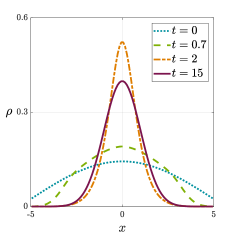
(a) Evolution of the density

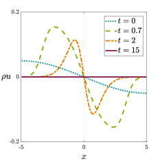
(b) Evolution of the momentum

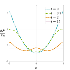
(c) Evolution of the variation of the free energy

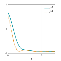
(d) Evolution of the total energy and free energy

Figure 1. Temporal evolution of Example 3.1.

Table 2. Accuracy test for Example 3.1 with the first and second-order schemes, at $t=0.3$

Number of cells	First-order		Second-order
	$L^{1}$ error	order	$L^{1}$ error	order
50	6.8797E-03	-	7.6166E-04	-
100	3.4068E-03	1.01	2.0206E-04	1.91
200	1.6826E-03	1.02	5.0308E-05	2.01
400	8.3104E-04	1.02	1.2879E-05	1.97

Example 3.2 (Ideal-gas pressure, attractive potential and Cucker-Smale damping terms).

In this example the pressure satisfies $P(\rho)=\rho$ and there is an external potential of the form $V(x)=\frac{x^{2}}{2}$. The difference with example 3.1 is that the Cucker-Smale damping terms are included, and the linear damping term $-\rho u$ excluded.

The relation holding in the steady state is expressed in (46) and the steady state satisfies (47). The initial conditions are also (48). The order of accuracy test from this example is shown in table 3, and the evolution of the density, momentum, variation of the free energy with respect to the density, total energy and free energy are depicted in figure 2. The lack of linear damping leads to higher oscillations in the momentum plots in comparison to figure 1. There is also an exchange of kinetic and free energy during the temporal evolution, which could be noticed from the oscillations of the discrete free energy in figure 2 (D).

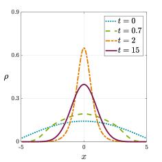
(a) Evolution of the density

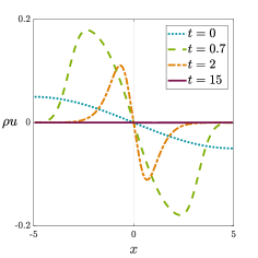
(b) Evolution of the momentum

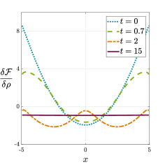
(c) Evolution of the variation of the free energy

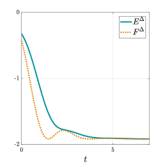
(d) Evolution of the total energy and free energy

Figure 2. Temporal evolution of Example 3.2.

Table 3. Accuracy test for Example 3.2 with the first and second-order schemes, at $t=0.3$

Number of cells	First-order		Second-order
	$L^{1}$ error	order	$L^{1}$ error	order
50	6.3195E-03	-	7.3045E-04	-
100	3.2658E-03	0.95	1.9462E-04	1.91
200	1.6373E-03	1.00	4.8629E-05	2.00
400	8.7771E-04	1.01	1.2468E-05	1.97

Example 3.3 (Ideal-gas pressure and attractive kernel).

In this case study the pressure satisfies $P(\rho)=\rho$ and there is an interaction potential with a kernel of the form $W(x)=\frac{x^{2}}{2}$. The steady state for a general total mass $M_{0}$ is again equal to the steady states from examples 3.1 and 3.2 with unit mass. The linear damping coefficient $\gamma$ has been reduced, $\gamma=0.01$, in order to compare the evolution with respect to the previous examples.

The initial conditions for the order of accuracy test are the ones from example 3.1 in (48). The order of accuracy test from this example is shown in table 4, and the evolution of the density, momentum, variation of the free energy with respect to the density, total energy and free energy are depicted in figure 3. Due to the low value of $\gamma$ in the linear damping, there is a repeated exchange of free energy and kinetic energy during the temporal evolution, which can be noticed from the oscillations of the free energy plot in figure 3 (D). In the previous examples the linear damping term dissipates the momentum in a faster timescale and these exchanges only last for a few oscillations. One can also notice that the time to reach the steady state is higher than in the previous examples.

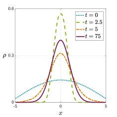
(a) Evolution of the density

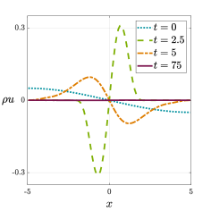
(b) Evolution of the momentum

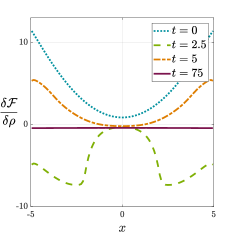
(c) Evolution of the variation of the free energy

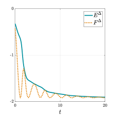
(d) Evolution of the total energy and free energy

Figure 3. Temporal evolution of Example 3.3.

Table 4. Accuracy test for Example 3.3 with the first and second-order schemes, at $t=0.3$

Number of cells	First-order		Second-order
	$L^{1}$ error	order	$L^{1}$ error	order
50	6.6938E-03	-	7.6135E-04	-
100	3.4702E-03	0.95	2.0207E-04	1.91
200	1.7410E-03	1.00	5.0306E-05	2.01
400	8.6890E-04	1.00	1.2879E-05	1.97

Example 3.4 (Pressure proportional to square of density and attractive potential).

For this example the pressure satisfies $P(\rho)=\rho^{2}$ and there is an external potential of the form $V(x)=\frac{x^{2}}{2}$. Contrary to the previous examples 3.1, 3.2 and 3.3, the choice of $P(\rho)=\rho^{2}$ implies that regions of vacuum where $\rho=0$ appear in the evolution and steady solution of the system. As explained in the introduction of this section, the numerical flux employed for this case is a kinetic solver based on [6].

The steady state for this example with an initial mass of $M_{0}$ satisfies

$$\rho_{\infty}(x)=\left\{\begin{array}[]{ll}\displaystyle-\frac{1}{4}\left(x+\sqrt[3]{3M_{0}}\right)\left(x-\sqrt[3]{3M_{0}}\right)&\textrm{for}\quad x\in\left[-\sqrt[3]{3M_{0}},\sqrt[3]{3M_{0}}\right],\\[8.53581pt] 0&\textrm{otherwise}.\end{array}\right.$$

The initial conditions taken for the order of accuracy test are

$$\rho(x,t=0)=M_{0}\frac{0.1+e^{-x^{2}}}{\int_{\mathbb{R}}\left(0.1+e^{-x^{2}}\right)dx},\quad\rho u(x,t=0)=-0.2\sin\left(\frac{\pi x}{10}\right),\quad x\in[-5,5],$$

with $M_{0}$ being the mass of the system and equal to $1$. The order of accuracy test from this example is shown in table 5, and the evolution of the density, momentum, variation of the free energy with respect to the density, total energy and free energy are depicted in figure 4. The initial kinetic energy represents a large part of the initial total energy, and there is also an exchange between the kinetic energy and the free energy resulting in the oscillations for the plot of the discrete free energy.

As a remark, in this example the order of accuracy for the schemes with order higher than one is reduced to one both in the vacuum and interface regions, as it is also pointed out in [27]. The orders showed in table 5 are computed by considering only the cells in the support of the density that are away from the interface region, and the vacuum regions are not taken into consideration.

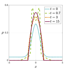
(a) Evolution of the density

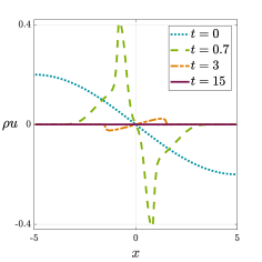
(b) Evolution of the momentum

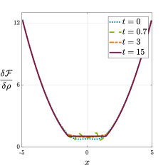
(c) Evolution of the variation of the free energy

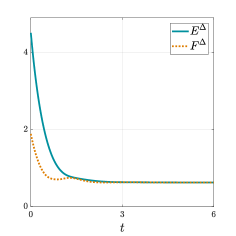
(d) Evolution of the total energy and free energy

Figure 4. Temporal evolution of Example 3.4.

Table 5. Accuracy test for Example 3.4 with the first and second-order schemes, at $t=0.3$

Number of cells	First-order		Second-order
	$L^{1}$ error	order	$L^{1}$ error	order
50	6.8826E-03	-	1.0735E-03	-
100	3.5106E-03	0.97	2.9188E-04	1.88
200	1.7596E-03	1.00	7.6113E-05	1.94
400	8.8184E-04	1.00	1.9103E-05	1.99

Example 3.5 (Moving steady state with ideal-gas pressure, attractive kernel and Cucker-Smale damping term).

The purpose of this example is to show that our scheme from section 2 preserves the order of accuracy for moving steady states of the form (12), where the velocity is not dissipated. As mentioned in the introduction, the generalization of well-balanced schemes to preserve moving steady states has proven to be quite complicated [58, 76], and it is not the aim of this work to construct such schemes.

For this example the pressure satisfies $P(\rho)=\rho$ and there is an interaction potential with a kernel of the form $W(x)=\frac{x^{2}}{2}$. The linear damping is eliminated and the Cucker-Smale damping term included. Under this configuration, there exists an explicit solution for system (5) consisting in a travelling wave of the form

(49) $$\rho(x,t)=M_{0}\frac{e^{-(x-ut)^{2}/2}}{\int_{\mathbb{R}}e^{-x^{2}/2}dx},\quad u(x,t)=0.2,$$

with $M_{0}$ equals to $1$ so that the total mass is unitary. As a result, the order of accuracy test can be accomplished by computing the error with respect to the exact reference solution, contrary to what was proposed in the previous examples. It should be remarked however that the velocity and the variation of the free energy with respect to the density profiles are not kept constant along the domain by our numerical scheme, since the well-balanced property for moving steady states is not satisfied.

The initial conditions for our simulation are (49) at $t=0$, in a numerical domain with $x\in[-8,9]$. The simulation is run until $t=3$. The table of errors for different number of cells is showed in table 6, and a depiction of the evolution of the system is illustrated in figure 5. The velocity and the variation of the free energy plots are not included since they are not maintained constant with our scheme.

Table 6. Accuracy test for Example 3.5 with the first and second-order schemes, at $t=3$

Number of cells	First-order		Second-order
	$L^{1}$ error	order	$L^{1}$ error	order
50	9.84245E-03	-	2.78988E-03	-
100	4.92029E-03	1.00	9.09342E-04	1.62
200	2.44627E-03	1.01	2.55340E-04	1.83
400	1.21228E-03	1.01	7.47905E-05	1.77

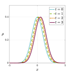
(a) Evolution of the density

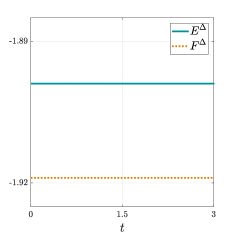
(b) Evolution of the total energy and free energy

Figure 5. Temporal evolution of Example 3.5.

3.2. Numerical experiments

This subsection applies the well-balanced scheme in section 2 to a variety of free energies from systems which have acquired an important consideration in the literature. Some of these systems have been mainly studied in their overdamped form, resulting when $\gamma\to\infty$, and as a result our well-balanced scheme can be useful in determining the role that inertia plays in those systems.

Example 3.6 (Pressure proportional to square of density and double-well potential).

In this example the pressure is taken as in example 3.4, with $P(\rho)=\rho^{2}$, thus leading to vacuum regions. The external potential are chosen to have a double-well shape of the form $V(x)=a\,x^{4}-b\,x^{2}$, with $a,\,b>0$. This system exhibits a variety of steady states depending on the symmetry of the initial condition, the initial mass and the shape of the external potential $V(x)$. The general expression for the steady states is

$$\rho_{\infty}=\left(C(x)-V(x)\right)_{+}=\left(C(x)-a\,x^{4}+b\,x^{2}\right)_{+},$$

where $C(x)$ is a piecewise constant function, zero outside the support of the density. Notice that $C(x)$ can attain a different value in each connected component of the support of the density.

Three different initial data are simulated in order to compare the resulting long time asymptotics, i.e., we show that different steady states are achieved corresponding to different initial data. The initial conditions are

$$\rho(x,t=0)=M_{0}\frac{0.1+e^{-(x-x_{0})^{2}}}{\int_{\mathbb{R}}\left(0.1+e^{-(x-x_{0})^{2}}\right)dx},\quad\rho u(x,t=0)=-0.2\sin\left(\frac{\pi x}{10}\right),\quad x\in[-10,10],$$

with $M_{0}$ equal to $1$ so that the total mass is unitary. When $x_{0}=0$, the initial density is symmetric, and when $x_{0}\neq 0$ the initial density is asymmetric.

1. First case: The external potential satisfies $V(x)=\frac{x^{4}}{4}-\frac{3x^{2}}{2}$ and the initial density is symmetric with $x_{0}=0$. For this configuration the steady solution presents two disconnected bumps of density with the same mass in each of them, as it is shown in figure 6 (A) and (B). The variation of the free energy with respect to the density presents the same constant value in the two disconnected supports of the density. The evolution is symmetric throughout.

   

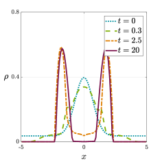
   (a) Density in first case

   

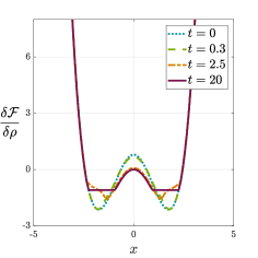
   (b) Variation of the free energy in first case

   

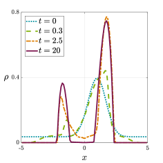
   (c) Density in second case

   

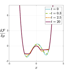
   (d) Evolution of the variation of the free energy in second case

   

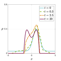
   (e) Density in third case

   

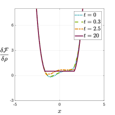
   (f) Variation of the free energy in third case

   Figure 6. Temporal evolution of the first, second and third cases from example 3.6.

2. Second case: The external potential satisfies $V(x)=\frac{x^{4}}{4}-\frac{3x^{2}}{2}$ and the initial density is asymmetric with $x_{0}=1$. The final steady density is characterised again by the two disconnected supports but for this configuration the mass in each of them varies, as shown in figure 6 (C) and (D). Similarly, the variation of the free energy with respect to the density presents different constant values in the two disconnected supports of the density.

3. Third case: for this last configuration the external potential is varied and satisfies $V(x)=\frac{x^{4}}{4}-\frac{x^{2}}{2}$, and the initial density is asymmetric with $x_{0}=1$. For this case, even though the initial density is asymmetric, the final steady density is symmetric and compactly supported due to the shape of the potential, as it is shown in figure 6 (E) and (F). The variation of the free energy with respect to the density presents constant value in all the support of the density.

This behavior shows that this problem has a complicated bifurcation diagram and corresponding stability properties depending on the parameters, for instance the coefficient on the potential well controling the depth and support of the wells used above.

Example 3.7 (Ideal pressure with noise parameter and its phase transition).

The model proposed for this example has a pressure satisfying $P(\rho)=\sigma\rho$, where $\sigma$ is a noise parameter, and external and interaction potentials chosen to be $V(x)=\frac{x^{4}}{4}-\frac{x^{2}}{2}$ and $W(x)=\frac{x^{2}}{2}$, respectively. The corresponding model in the overdamped limit has been previously studied in the context of collective behaviour [3], mean field limits [35], and systemic risk [30], see also [70] for the proof in one dimension.

We find that this hydrodynamic system exhibits a supercritical pitchfork bifurcation in the center of mass $\hat{x}$ of the steady state when varying the noise parameter $\sigma$ as its overdamped limit counterpart discussed above. For values of $\sigma$ higher than a certain threshold, all teady states are symmetric and have the center of mass $\hat{x}$ at $x=0$. However, when $\sigma$ decreases below that threshold, the pitchfork bifurcation takes place. On the one hand, if the center of mass of the initial density is at $x=0$, the final center of mass in the steady state remains at $x=0$. On the other hand, if the center of mass of the initial density is at $x\neq 0$, the center of mass of the steady state approaches asymptotically to $x=1$ or $x=-1$ as $\sigma\to 0$, depending on the sign of the initial center of mass. Finally, when $\sigma=0$, the steady state turns into a Dirac delta at $x=0$, $x=1$ or $x=-1$, depending on the initial density.

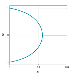
(a) Bifurcation diagram

 

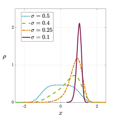
(b) Steady state profiles for different $\sigma$

Figure 7. Bifurcation diagram (A) and steady states for different values of the noise parameter $\sigma$ (B) from Example 3.7

The pitchfork bifurcation is supercritical since the branch of the bifurcation corresponding to $\hat{x}=0$ is unstable. This means that any deviation from an initial center of mass at $x=0$ leads to a steady center of mass located in one of the two branches of the parabola in the bifurcation state.

The numerical scheme outlined in section 2 captures this bifurcation diagram for the evolution of the hydrodynamic system. The results are shown in figure 7. In it, (A) depicts the bifurcation diagram of the final centre of mass when the noise parameter $\sigma$ is varied, and for an initial center of mass at $x\neq 0$. For a symmetric initial density and antisymmetric velocity, the centre of mass numerically remains at $x=0$ for an adequate stopping criterion, since property (vi) in subsection 2.2 holds. However, any slight error in the numerical computation unavoidably leads to a steady state deviating towards any of the two stable branches, due to the strong unstable nature of the branch with $x=0$. In (B) of figure 7 there is an illustration of the steady states resulting from an initial center of mass located at $x>0$, for different choices of the noise parameter $\sigma$. For $\sigma=0.001$, which is the smallest value of $\sigma$ simulated, the density profile approaches the theoretical Dirac delta expected at $x=1$ when $\sigma\to 0$. When $\sigma=0$ the hyperbolicity of the system in (5) is lost since the pressure term vanishes, and as a result the numerical approach in section 2 cannot be applied.

The numerical strategy followed to recover the bifurcation diagram is based on the so-called differential continuation. It simply means that, as $\sigma\to 0$, the subsequent simulations with new and lower values of $\sigma$ have as initial conditions the previous steady state from the last simulation. This allows to complete the bifurcation diagram, since otherwise the simulations with really small $\sigma$ take long time to converge for general initial conditions. In addition, to maintain sufficient resolution for the steady states close to the Dirac delta, the mesh is adapted for each simulation. This is accomplished by firstly interpolating the previous steady state with a piecewise cubic hermite polynomial, which preserves the shape and avoids oscillations, and secondly by creating a new and narrower mesh where the interpolating polynomial is employed to construct the new initial condition for the differential continuation.

Example 3.8 (Hydrodynamic generalization of the Keller-Segel system - Generalized Euler-Poisson systems).

The original Keller-Segel model has been widely employed in chemotaxis, which is usually defined as the directed movement of cells and organisms in response to chemical gradients [47]. These systems also find their applications in astrophysics and gravitation [67, 24]. It is a system of two coupled drift-diffusion differential equations for the density $\rho$ and the chemoattractant concentration $S$,

$$\begin{cases}{\displaystyle\partial_{t}\rho=\nabla\cdot\left(\nabla P(\rho)-\chi\rho\nabla S\right),}\\[5.69054pt] {\displaystyle\partial_{t}S=D_{s}\Delta S-\theta S+\beta\rho.}\end{cases}$$

In this system $P(\rho)$ is the pressure, and the biological/physical meaning of the constants $\chi$, $D_{s}$, $\alpha$ and $\beta$ can be reviewed in the literature [42, 4, 41]. For this example they are simplified as usual so that $\chi=D_{s}=\beta=1$ and $\theta=0$. A further assumption usually taken in the literature is that $\partial_{t}\rho$ is very big in comparison to $\partial_{t}S$ [41], leading to a simplification of the equation for the chemoattractant concentration $S$, which becomes the Poisson equation $-\Delta S=\rho$. Hydrodynamic extensions of the model, which include inertial effects, have also been proven to be essential for certain applications[19, 20, 29], leading to a hyperbolic system of equations with linear damping which in one dimension reads as

$$\begin{cases}\partial_{t}\rho+\partial_{x}\left(\rho u\right)=0,\\[5.69054pt] {\displaystyle\partial_{t}(\rho u)\!+\partial_{x}(\rho u^{2})\!=-\partial_{x}P(\rho)+\partial_{x}S-\gamma\rho u,}\\[5.69054pt] {-\partial_{xx}S=\rho.}\end{cases}$$

By using the fundamental solution of the Laplacian in one dimension, this equation becomes $2S=|x|\star\rho$. This term, after neglecting the constant, can be plugged in the momentum equation so that the last equation for $S$ can be removed. As a result, the hydrodynamic Keller-Segel model is reduced to the system of equations (1) considered in this work, with $W(x)=|x|/2$, $V(x)=0$ and $\psi\equiv 0$. As a final generalization [10], the original interaction potential $W(x)=|x|/2$ can be extended to be a homogeneous kernel $W(x)=|x|^{\alpha}/\alpha$, where $\alpha>-1$. By convention, $W(x)=\ln|x|$ for $\alpha=0$. Further generalizations are Morse-like potentials as in [17, 10] where $W(x)=1-\exp(-|x|^{\alpha}/\alpha)$ with $\alpha>0$.

The solution of this system can present a rich variety of behaviours due to the competition between the attraction from the local kernel $W(x)$ and the repulsion caused by the diffusion of the pressure $P(\rho)$, as reviewed in [7, 8]. By appropriately tuning the parameters $\alpha$ in the kernel $W(x)$ and $m$ in the pressure $P(\rho)$, one can find compactly supported steady states, self-similar behavior, or finite-time blow up. Three different regimes have been studied in the overdamped generalized Keller-Segel model [10]: diffusion dominated regime ($m>1-\alpha$), balanced regime ($m=1-\alpha$) where a critical mass separates self-similar and blow-up behaviour, and aggregation-dominated regime ($m<1-\alpha$). These three regimes have not been so far analytically studied for the hydrodynamic system except for few particular cases [12, 13], and the presence of inertia indicates that the initial momentum profile plays a role together with the mass of the system to separate diffusive from blow-up behaviour.

The well-balanced scheme provided in section 2 is a useful tool to effectively reach the varied steady states resulting from different values of $\alpha$ and $m$. The objective of this example is to provide some numerical experiments to show the richness of possible behaviors. This scheme can be eventually employed to numerically validate the theoretical studies concerning the existence of the different regimes for the hydrodynamic system for instance, or how the choice of the initial momentum or the total mass can lead to diffusive or blow-up behaviour. This will be explored further elsewhere.

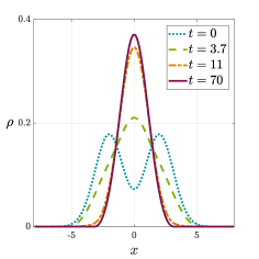
(a) Evolution of the density

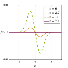
(b) Evolution of the momentum

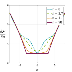
(c) Evolution of the variation of the free energy

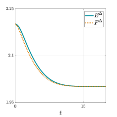
(d) Evolution of the total energy and free energy

Figure 8. Temporal evolution of Example 3.8 with compactly-supported steady state.

We have conducted two simulations with different choices of the paramenters $\alpha$ and $m$. In both $m>1$, so that a proper numerical flux able to deal with vacuum regions has to be implemented. As emphasised in the introduction of this section, the kinetic scheme developed in [63] is employed. Both of the simulations share the same initial conditions,

$$\rho(x,t=0)=M_{0}\frac{e^{-\frac{4(x+2)^{2}}{10}}+e^{-\frac{4(x-2)^{2}}{10}}}{\int_{\mathbb{R}}\left(e^{-\frac{4(x-2)^{2}}{10}}+e^{-\frac{4(x+2)^{2}}{10}}\right)dx},\quad\rho u(x,t=0)=0,\quad x\in[-8,8],$$

where the total mass $M_{0}$ of the system is $1$.

In the first simulation the choice of parameters is $\alpha=0.5$ and $m=1.5$. According to the regime classification for the overdamped system, this would correspond to the diffusion-dominated regime. In the overdamped limit, solutions exist globally in time, and the steady state is compactly supported. The results are depicted in figure 8 and adequately agree with this regime. In the steady state the variation of the free energy with respect to density has a constant value only in the support of the density, as expected. The total energy decreases in time and there is no exchange between the free energy and the kinetic energy since the free energy in figure 8 (D) does not oscillate.

 

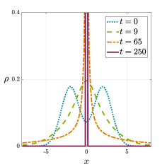
(a) Evolution of the density

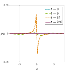
(b) Evolution of the momentum

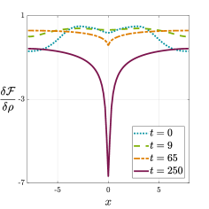
(c) Evolution of the variation of the free energy

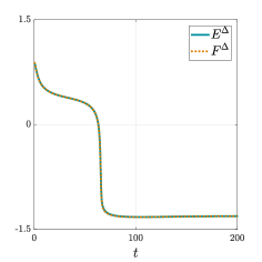
(d) Evolution of the total energy and free energy

Figure 9. Temporal evolution of Example 3.8 with finite-time blow up.

The second simulation has a choice of parameters of $\alpha=-0.5$ and $m=1.3$. In the case of the overdamped system this would correspond to the aggregation-dominated regime, where blow-up and diffusive behaviour coexist and depend on the initial density profile. The results from this simulation of the hydrodynamic system are illustrated in figure 9. For this particular initial condition there is analytically finite-time blow up. Our scheme, due to the conservation of mass of the finite volume scheme, concentrates all the mass in one single cell in finite time, that is, the scheme achieves in finite time the better approximation to a Dirac Delta at a point with the chosen mesh. Once this happens, this artificial numerical steady state depending on the mesh is kept for all times. From figure 9 (C) it is evident that the variation of the free energy with respect to density does not reach a constant value, and in figure 9 (D) the free energy presents a sharp decay when the concentration in one cell is produced (around $t\approx 65$). The value of the slope in the free energy plot theoretically tends to $-\infty$ due to the blow up, but in the simulation the decay is halted due to conservation of mass and the artificial steady state. This agrees with the fact that the expected Dirac delta profile in the density at the blow up time is obviously not reached numerically. It was also checked that this phenomena repeats for all meshes leading to more concentrated artificial steady states with more negative free energy values for more refined meshes. For other more spreaded initial conditions our scheme produces diffusive behaviour as expected from theoretical considerations.

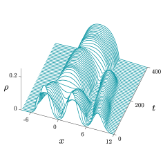
(a) Evolution of the density

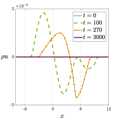
(b) Evolution of the momentum

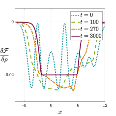
(c) Evolution of the variation of the free energy

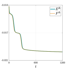
(d) Evolution of the total energy and free energy

Figure 10. Temporal evolution of Example 3.8 with Morse-type potential and three initial density bumps.

A further simulation is carried out to explore the convergence in time towards equilibration with a Morse-type potential of the form $W(x)=-e^{-|x|^{2}/2}/\sqrt{2\pi}$. With this potential the attraction between two bumps of density separated at a considerable distance is quite small. However, when enough time has passed and the bumps get closer, they merge in an exponentially fast pace due to the convexity of the Gaussian potential, and a new equilibrium is reached with just one bump. The interesting fact about this system is therefore the existence of two timescales: the time to get the bumps of density close enough, which could be arbitrarily slow, and the time to merge the bumps, which is exponentially fast in time.

We have set up a simulation whose initial state presents three bumps of density, with the initial conditions satisfying

$$\rho(x,t=0)=M_{0}\frac{e^{-\frac{(x+3)^{2}}{2}}+e^{-\frac{(x-3)^{2}}{2}}+0.55e^{-\frac{(x-8.5)^{2}}{2}}}{\int_{\mathbb{R}}\left(e^{-\frac{(x+3)^{2}}{2}}+e^{-\frac{(x-3)^{2}}{2}}+0.55e^{-\frac{(x-8.5)^{2}}{2}}\right)dx},\quad\rho u(x,t=0)=0,\quad x\in[-8,12],$$

and the total mass of the system equal to $M_{0}=1.2$. The parameter $m$ in the pressure satisfies $m=3$, and the effect of the linear damping is reduced by assigning $\gamma=0.05$.

The results are depicted in 10. In (A) one can observe how the two central bumps of density merge after some time, and how the third bump, with less mass, starts getting closer in time until it also blends. This is also reflected in the evolution of the free energy in figure 10 (D), where there are two sharp and exponential decays corresponding to the merges of the bumps.

Example 3.9 (DDFT for 1D hard rods).

Classical (D)DFT is a theoretical framework provided by nonequilibrium statistical mechanics but has increasingly become a widely-employed method for the computational scrutiny of the microscopic structure of both uniform and non-uniform fluids [25, 33, 78, 79, 54]. The DDFT equations have the same form as in (5) when the hydrodynamic interactions are neglected. The starting point in (D)DFT is a functional $\mathcal{F}[\rho]$ for the fluid’s free energy which encodes all microscopic information such as the ideal-gas part, short-range repulsive effects induced by molecular packing, attractive interactions and external fields. This functional can be exactly derived only for a limited number of applications, for instance the one-dimensional hard rod system from Percus [61]. However, in general it has to be approximated by making appropriate assumptions, as e.g. in the so-called fundamental-measure theory of Rosenfeld [65]. These assumptions are usually validated by carrying out appropriate test simulations (e.g. of the underlying stochastic dynamics) to compare e.g. the DDFT system with the approximate free-energy functional to the microscopic reference system [32].

The objective of this example is to show that the numerical scheme in section 2 can also be applied to the physical free-energy functionals employed in (D)DFT, which satisfy the more complex expression for the free energy described in (13), and with a variation satisfying (14). For this example the focus is on the hard rods system in one dimension. Its free energy has a part depending on the local density and which satisfies the classical form for an ideal gas, with $P(\rho)=\rho$. It is therefore usually denoted as the ideal part of the free energy,

$$\mathcal{F}_{id}[\rho]=\int\Pi(\rho)dx=\int\rho(x)\left(\ln\rho-1\right)dx.$$

There is also a part of general free energy in (13) which contains the non-local dependence of the density, and has different exact or approximative forms depending of the system under consideration. In (D)DFT it is denoted as the excessive free energy, and for the hard rods satisfies

$$\mathcal{F}_{ex}[\rho] =\frac{1}{2}\int K\left(W(\bm{x})\star\rho(\bm{x})\right)\rho(\bm{x})d\bm{x}$$

$$=-\frac{1}{2}\int\rho(x+\sigma/2)\ln\left(1-\eta(x)\right)dx-\frac{1}{2}\int\rho(x-\sigma/2)\ln\left(1-\eta(x)\right)dx,$$

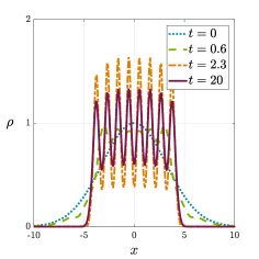
(a) Evolution of the density

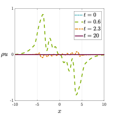
(b) Evolution of the momentum

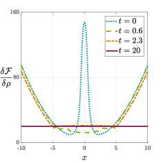
(c) Evolution of the variation of the free energy

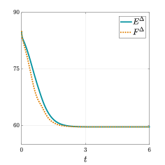
(d) Evolution of the total energy and free energy

Figure 11. Temporal evolution of Example 3.9 with $8$ hard rods and a confining potential.

where $\sigma$ is the length of a hard rod and $\eta(x)$ the local packing fraction representing the probability that a point $x$ is covered by a hard rod,

$$\eta(x)=\int_{-\frac{\sigma}{2}}^{\frac{\sigma}{2}}\rho(x+y)dy.$$

The function $K(x)$ in this case satisfies $K(x)=\ln(1-x)$ and the kernel $W(x)$ takes the form of a characteristic function which limits the interval of the packing function (3.9). To obtain the excessive free energy for the hard rods one has to also consider changes of variables in the integrals. The last part of the general free energy in (13) corresponds to the effect of the external potential $V(x)$. On the whole, the variation of the free energy in (13) with respect to the density, for the case of hard rods, satisfies

$$\frac{\delta\mathcal{F}[\rho]}{\delta\rho}= \frac{\delta\mathcal{F}_{id}[\rho]}{\delta\rho}+\frac{\delta\mathcal{F}_{ex}[\rho]}{\delta\rho}+V(x)$$

$$= \ln(\rho)-\frac{1}{2}\ln\left(1-\int_{x-\sigma}^{x}\rho(y)dy\right)-\frac{1}{2}\ln\left(1-\int_{x}^{x+\sigma}\rho(y)dy\right)$$

$$+\frac{1}{2}\int_{x-\sigma/2}^{x+\sigma/2}\left(\frac{\rho(x+\sigma/2)+\rho(x-\sigma/2)}{1-\eta(x)}\right)dx+V(x).$$

This system can be straightforwardly simulated with the well-balanced scheme from section 2 by gathering the excessive part of the free energy and the external potentials under the term $H(x,\rho)$, so that

$$H(x,\rho)=\frac{\delta\mathcal{F}_{ex}[\rho]}{\delta\rho}+V(x).$$

The first simulation seeks to capture the steady state reached by $8$ hard rods of unitary mass and length $\sigma=1$ under the presence of an external potential of the form $V(x)=x^{2}$. The initial conditions of the simulation are

$$\rho(x,t=0)=e^{-\frac{x^{2}}{20.372}},\quad\rho u(x,t=0)=0,\quad x\in[-13,13],$$

where the density is chosen so that the total mass of the system is $8$. The results are plotted in figure 11. The steady state reached for the density reveals layering due to the confining effects of the external potential and the repulsion between the hard rods. These layering effects can be amplified by increasing the coefficient in the external potential. It is also observed how each of the $8$ peaks has a unitary width. This is due to the fact that the length of the hard rods $\sigma$ was taken as $1$. The variation of the free energy with respect to the density also reaches a constant value in all the domain. For microscopic simulations of the underlying stochastic dynamics for similar examples we refer the reader to [33].

Starting from this last steady state, the second simulation performed for this example shows how the hard rods diffuse when the confining potential is removed. This simulation has as initial condition the previous steady state from figure 11 and the external potential is set to $V(x)=0$. The results are depicted in figure 12, and they share the same features of the simulations in [56]. The final steady state of the density is uniform profile resultant from the diffusion of the hard rods, and in this situation the variation of the free energy with respect to the density also reaches a constant value in the steady state, as expected.

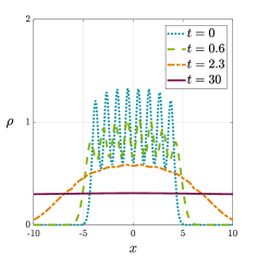
(a) Evolution of the density

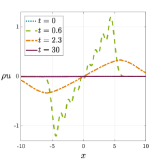
(b) Evolution of the momentum

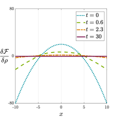
(c) Evolution of the variation of the free energy

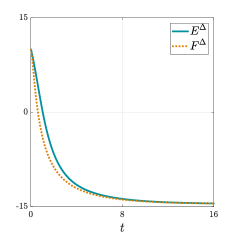
(d) Evolution of the total energy and free energy

Figure 12. Temporal evolution of Example 3.9 with $8$ hard rods and no potential.

4. Conclusions

We have introduced first- and second-order accurate finite volume schemes for a large family of hydrodynamic equations with general free energy, positivity preserving and free energy decaying properties. These hydrodynamic models with damping naturally arise in dynamic density functional theories and the accurate computation of their stable steady states is crucial to understand their phase transitions and stability properties. The models possess a common variational structure based on the physical free energy functional from statistical mechanics. The numerical schemes proposed capture very well steady states and their equilibration dynamics due to the crucial free energy decaying property resulting into well-balanced schemes. The schemes were validated in well-known test cases and the chosen numerical experiments corroborate these conclusions for intricate phase transitions and complicated free energies.

There are also several new avenues of possible future directions. Indeed, we believe the computational framework and associated methodologies presented here can be useful for the study of bifurcations and phase transitions for systems where the free energy is known from experiments only, either physical or in-silico ones, and then our framework can be adopted in a “data-driven” approach. Of particular extension would also be extension to multi-dimensional problems. Two-dimensional problems in particular would be of direct relevance to surface diffusion and therefore to technological processes in materials science and catalysis. We shall examine these and related problems in future studies.

Appendix A Numerical flux, temporal scheme, and CFL condition employed in the numerical simulations

This appendix aims to present the necessary details to compute the numerical flux, boundary conditions, the CFL condition, and the temporal discretization for the simulations in section 3.

The pressure function in the simulations has the form of $P(\rho)=\rho^{m}$, with $m\geq 1$. When $m=0$ the pressure satisfies the ideal-gas relation $P(\rho)=\rho$, and the density does not present vacuum regions during the temporal evolution. For this case the employed numerical flux is the versatile local Lax-Friedrich flux, which approximates the flux at the boundary $F_{i+\frac{1}{2}}$ in (17) as

(50) $$F_{i+\frac{1}{2}}=\mathscr{F}\left(U_{i+\frac{1}{2}}^{-},U_{i+\frac{1}{2}}^{+}\right)=\frac{1}{2}\left(F\left(U_{i+\frac{1}{2}}^{-}\right)+F\left(U_{i+\frac{1}{2}}^{+}\right)-\lambda_{i+\frac{1}{2}}\left(U_{i+\frac{1}{2}}^{+}-U_{i+\frac{1}{2}}^{-}\right)\right),$$

where $\lambda$ is taken as the maximum of the absolute value of the eigenvalues of the system,

(51) $$\lambda_{i+\frac{1}{2}}=\max_{\left(U_{i+\frac{1}{2}}^{-},U_{i+\frac{1}{2}}^{+}\right)}\left\{\left|u+\sqrt{P^{\prime}(\rho)}\right|,\left|u-\sqrt{P^{\prime}(\rho)}\right|\right\}.$$

This maximum is taken locally for every node, resulting in different values of $\lambda$ along the lines of nodes. It is also possible to take the maximum globally, leading to the classical Lax-Friedrich scheme.

For the simulations where $P(\rho)=\rho^{m}$ and $m>1$ vacuum regions with $\rho=0$ are generated. This implies that the hiperbolicity of the system (5) is lost in those regions, and the local Lax-Friedrich scheme fails. As a result, an appropiate numerical flux has to be implemented to handle the vacuum regions. In this case a kinetic solver based on [64] is employed. This solver is constructed from kinetic formalisms applied in macroscopic models, and has already been employed in previous works for shallow-water applications [2]. The flux at the boundary $F_{i+\frac{1}{2}}$ in (17) is computed from

(52) $$F_{i+\frac{1}{2}}=\mathscr{F}\left(U_{i+\frac{1}{2}}^{-},U_{i+\frac{1}{2}}^{+}\right)=A_{-}\left(U_{i+\frac{1}{2}}^{-}\right)+A_{+}\left(U_{i+\frac{1}{2}}^{+}\right),$$

where

(53) $$A_{-}\left(\rho,\rho u\right)=\int_{\xi\geq 0}\xi\begin{pmatrix}1\\ \xi\end{pmatrix}M(\rho,u-\xi)\,d\xi,\quad A_{+}\left(\rho,\rho u\right)=\int_{\xi\leq 0}\xi\begin{pmatrix}1\\ \xi\end{pmatrix}M(\rho,u-\xi)\,d\xi.$$

The function $M(\rho,\xi)$ is chosen accordingly to the kinetic representation of the macroscopic system, and for this case satisfies

(54) $$M(\rho,\xi)=\rho^{\frac{2-m}{2}}\chi\left(\frac{\xi}{\rho^{\frac{m-1}{2}}}\right).$$

The function $\chi(\omega)$ can be chosen in different ways. For this simulations we simply take it as a characteristic function,

(55) $$\chi(\omega)=\frac{1}{\sqrt{12}}\mathbbm{1}_{\left\{\left|\omega\right|\leq\sqrt{3}\right\}},$$

although [64] presents other possible choices for $\chi(\omega)$. Further valid numerical fluxes able to treat vacuum, such as the Rusanov flux or the Suliciu relaxation solver, are reviewed in [6].

The boundary conditions are taken to be no flux both for the density and the momentum equations. As a result, the evaluation of the numerical fluxes (17) at the boundaries of the domain is taken as

(56) $$F_{i-\frac{1}{2}}=0\enspace\text{if}\>i=1\quad\text{and}\quad F_{i+\frac{1}{2}}=0\enspace\text{if}\>i=n.$$

The time discretization is acomplished by means of the third order TDV Runge-Kutta method [39]. From (15) we can define $L(U)$ as $L(U)=S(x,U)-\partial_{x}F(U)$, so that $\partial_{t}U=L(U)$. Then, the third order TDV Runge-Kutta temporal scheme to advance from $U^{n}$ to $U^{n+1}$ with a time step $\Delta t$ reads

$$U^{(1)} =U^{n}+\Delta tL\left(U^{n}\right),$$

$$U^{(2)} =\frac{3}{4}U^{n}+\frac{1}{4}U^{(1)}+\frac{1}{4}\Delta tL\left(U^{(1)}\right),$$

$$U^{n+1} =\frac{1}{3}U^{n}+\frac{2}{3}U^{(2)}+\frac{2}{3}\Delta tL\left(U^{(2)}\right).$$

The time step $\Delta t$ for the case of Lax-Friedrich flux is chosen from the CFL condition,

(57) $$\Delta t=\text{CFL}\frac{\min_{i}\Delta x_{i}}{\max_{\forall\left(U_{i+\frac{1}{2}}^{-},U_{i+\frac{1}{2}}^{+}\right)}\left\{\left|u+\sqrt{P^{\prime}(\rho)}\right|,\left|u-\sqrt{P^{\prime}(\rho)}\right|\right\}},$$

and the $\Delta t$ for the kinetic flux, with a function $\chi(\omega)$ as in (55), is chosen as

(58) $$\Delta t=\text{CFL}\frac{\min_{i}\Delta x_{i}}{\max_{\forall\left(U_{i+\frac{1}{2}}^{-},U_{i+\frac{1}{2}}^{+}\right)}\left\{|u|+3^{\frac{m-1}{4}}\right\}}.$$

The CFL number is taken as $0.7$ in all the simulations.

References

- [1] E. Audusse, F. Bouchut, M.-O. Bristeau, R. Klein, and B. t. Perthame, A fast and stable well-balanced scheme with hydrostatic reconstruction for shallow water flows, SIAM J. Sci. Comput., 25 (2004), pp. 2050–2065.
- [2] E. Audusse and M.-O. Bristeau, A well-balanced positivity preserving “second-order” scheme for shallow water flows on unstructured meshes, J. Comput. Phys., 206 (2005), pp. 311–333.
- [3] A. B. T. Barbaro, J. A. Canizo, J. A. Carrillo, and P. Degond, Phase Transitions in a Kinetic Flocking Model of Cucker–Smale Type, Multiscale Model. Simul., 14 (2016), pp. 1063–1088.
- [4] N. Bellomo, A. Bellouquid, Y. Tao, and M. Winkler, Toward a mathematical theory of Keller–Segel models of pattern formation in biological tissues, Math. Model. Methods Appl. Sci., 25 (2015), pp. 1663–1763.
- [5] A. Bermudez and M. E. Vázquez, Upwind methods for hyperbolic conservation laws with source terms, Comput. Fluids, 23 (1994), pp. 1049–1071.
- [6] F. Bouchut, Nonlinear stability of finite Volume Methods for hyperbolic conservation laws: And Well-Balanced schemes for sources, Springer Science & Business Media, 2004.
- [7] V. Calvez, J. A. Carrillo, and F. Hoffmann, Equilibria of homogeneous functionals in the fair-competition regime, Nonlinear Anal., 159 (2017), pp. 85–128.
- [8] V. Calvez, J. A. Carrillo, and F. Hoffmann, The geometry of diffusing and self-attracting particles in a one-dimensional fair-competition regime, in Nonlocal Nonlinear Diffus. Interact. New Methods Dir., Springer, 2017, pp. 1–71.
- [9] A. Canestrelli, A. Siviglia, M. Dumbser, and E. F. Toro, Well-balanced high-order centred schemes for non-conservative hyperbolic systems. Applications to shallow water equations with fixed and mobile bed, Adv. Water Resour., 32 (2009), pp. 834–844.
- [10] J. A. Carrillo, A. Chertock, and Y. Huang, A finite-volume method for nonlinear nonlocal equations with a gradient flow structure, Commun. Comput. Phys., 17 (2015), pp. 233–258.
- [11] J. A. Carrillo, Y.-P. Choi, and S. P. Perez, A review on attractive–repulsive hydrodynamics for consensus in collective behavior, in Act. Part. Vol. 1, Springer, 2017, pp. 259–298.
- [12] J. A. Carrillo, Y.-P. Choi, E. Tadmor, and C. Tan, Critical thresholds in 1D Euler equations with non-local forces, Math. Model. Methods Appl. Sci., 26 (2016), pp. 185–206.
- [13] J. A. Carrillo, Y.-P. Choi, and E. Zatorska, On the pressureless damped Euler–Poisson equations with quadratic confinement: Critical thresholds and large-time behavior, Math. Model. Methods Appl. Sci., 26 (2016), pp. 2311–2340.
- [14] J. A. Carrillo, K. Craig, and F. S. Patacchini, A blob method for diffusion, arXiv Prepr. arXiv1709.09195, (2017).
- [15] J. A. Carrillo, E. Feireisl, P. Gwiazda, and A. Świerczewska-Gwiazda, Weak solutions for Euler systems with non-local interactions, J. London Math. Soc., 95 (2017), pp. 705–724.
- [16] J. A. Carrillo, S. Hittmeir, B. Volzone, and Y. Yao, Nonlinear aggregation-diffusion equations: Radial symmetry and long time asymptotics, arXiv Prepr. arXiv1603.07767, (2016).
- [17] J. A. Carrillo, Y. Huang, and S. Martin, Explicit flock solutions for quasi-morse potentials, Eur. J. Appl. Math., 25 (2014), pp. 553–578.
- [18] J. A. Carrillo, A. Wróblewska-Kamińska, and E. Zatorska, On long-time asymptotics for viscous hydrodynamic models of collective behavior with damping and nonlocal interactions, arXiv Prepr. arXiv1709.09290, (2018).
- [19] P.-H. Chavanis, Jeans type instability for a chemotactic model of cellular aggregation, Eur. Phys. J. B-Condensed Matter Complex Syst., 52 (2006), pp. 433–443.
- [20] P.-H. Chavanis and C. Sire, Kinetic and hydrodynamic models of chemotactic aggregation, Phys. A Stat. Mech. its Appl., 384 (2007), pp. 199–222.
- [21] F. Cucker and S. Smale, Emergent behavior in flocks, IEEE Trans. Automat. Contr., 52 (2007), pp. 852–862.
- [22] , On the mathematics of emergence, Japanese J. Math., 2 (2007), pp. 197–227.
- [23] B. A. De Dios, J. A. Carrillo, and C.-W. Shu, Discontinuous Galerkin methods for the multi-dimensional Vlasov–Poisson problem, Math. Model. Methods Appl. Sci., 22 (2012), p. 1250042.
- [24] Y. Deng, T.-P. Liu, T. Yang, and Z.-a. Yao, Solutions of Euler-Poisson Equations for Gaseous Stars, Arch. Ration. Mech. Anal., 164 (2002), pp. 261–285.
- [25] M. A. Durán-Olivencia, B. D. Goddard, and S. Kalliadasis, Dynamical density functional theory for orientable colloids including inertia and hydrodynamic interactions, J. Stat. Phys., 164 (2016), pp. 785–809.
- [26] F. Filbet, P. Laurençot, and B. Perthame, Derivation of hyperbolic models for chemosensitive movement, J. Math. Biol., 50 (2005), pp. 189–207.
- [27] F. Filbet and C.-W. Shu, Approximation of hyperbolic models for chemosensitive movement, SIAM J. Sci. Comput., 27 (2005), pp. 850–872.
- [28] J. M. Gallardo, C. Parés, and M. Castro, On a well-balanced high-order finite volume scheme for shallow water equations with topography and dry areas, J. Comput. Phys., 227 (2007), pp. 574–601.
- [29] A. Gamba, D. Ambrosi, A. Coniglio, A. De Candia, S. Di Talia, E. Giraudo, G. Serini, L. Preziosi, and F. Bussolino, Percolation, morphogenesis, and Burgers dynamics in blood vessels formation, Phys. Rev. Lett., 90 (2003), p. 118101.
- [30] J. Garnier, G. Papanicolaou, and T.-W. Yang, Large deviations for a mean field model of systemic risk, SIAM J. Financ. Math., 4 (2013), pp. 151–184.
- [31] J. Giesselmann, C. Lattanzio, and A. E. Tzavaras, Relative energy for the Korteweg theory and related Hamiltonian flows in gas dynamics, Arch. Ration. Mech. Anal., 223 (2017), pp. 1427–1484.
- [32] B. D. Goddard, A. Nold, N. Savva, G. A. Pavliotis, and S. Kalliadasis, General dynamical density functional theory for classical fluids, Phys. Rev. Lett., 109 (2012), p. 120603.
- [33] B. D. Goddard, A. Nold, N. Savva, P. Yatsyshin, and S. Kalliadasis, Unification of dynamic density functional theory for colloidal fluids to include inertia and hydrodynamic interactions: derivation and numerical experiments, J. Phys. Condens. Matter, 25 (2012), p. 35101.
- [34] B. D. Goddard, G. A. Pavliotis, and S. Kalliadasis, The overdamped limit of dynamic density functional theory: Rigorous results, Multiscale Model. Simul., 10 (2012), pp. 633–663.
- [35] S. N. Gomes and G. A. Pavliotis, Mean field limits for interacting diffusions in a two-scale potential, J. nonlinear Sci., 28 (2018), pp. 905–941.
- [36] L. Gosse, Asymptotic-preserving and well-balanced schemes for the 1D Cattaneo model of chemotaxis movement in both hyperbolic and diffusive regimes, J. Math. Anal. Appl., 388 (2012), pp. 964–983.
- [37] , Computing qualitatively correct approximations of balance laws, vol. 2, Springer, 2013.
- [38] L. Gosse and A.-Y. Leroux, A well-balanced scheme designed for inhomogeneous scalar conservation laws, Comptes Rendus L Acad. Des Sci. Ser. I-mathematique, 323 (1996), pp. 543–546.
- [39] S. Gottlieb and C.-W. Shu, Total variation diminishing Runge-Kutta schemes, Math. Comput. Am. Math. Soc., 67 (1998), pp. 73–85.
- [40] J. M. Greenberg and A.-Y. LeRoux, A well-balanced scheme for the numerical processing of source terms in hyperbolic equations, SIAM J. Numer. Anal., 33 (1996), pp. 1–16.
- [41] F. Hoffmann, Keller-Segel-Type Models and Kinetic Equations for Interacting Particles: Long-Time Asymptotic Analysis, PhD thesis, University of Cambridge, 2017.
- [42] D. Horstmann and Others, From 1970 until present: the Keller-Segel model in chemotaxis and its consequences, (2003).
- [43] G.-S. Jiang and C.-W. Shu, Efficient implementation of weighted ENO schemes, J. Comput. Phys., 126 (1996), pp. 202–228.
- [44] T. Katsaounis, B. Perthame, and C. Simeoni, Upwinding sources at interfaces in conservation laws, Appl. Math. Lett., 17 (2004), pp. 309–316.
- [45] T. Katsaounis and C. Simeoni, Second order approximation of the viscous saint-venant system and comparison with experiments, in Hyperbolic Problems: Theory, Numerics, Applications, Springer, 2003, pp. 633–644.
- [46] , First and second order error estimates for the upwind source at interface method, Mathematics of computation, 74 (2005), pp. 103–122.
- [47] E. F. Keller and L. A. Segel, Initiation of slime mold aggregation viewed as an instability, J. Theor. Biol., 26 (1970), pp. 399–415.
- [48] A. Kurganov, G. Petrova, and Others, A second-order well-balanced positivity preserving central-upwind scheme for the Saint-Venant system, Commun. Math. Sci., 5 (2007), pp. 133–160.
- [49] A. Lasota and M. C. Mackey, Chaos, fractals, and noise: stochastic aspects of dynamics, vol. 97, Springer Science & Business Media, 2013.
- [50] A. Y. Leroux, Riemann solvers for some hyperbolic problems with a source term, in ESAIM Proc., vol. 6, EDP Sciences, 1999, pp. 75–90.
- [51] R. J. LeVeque, Balancing source terms and flux gradients in high-resolution Godunov methods: the quasi-steady wave-propagation algorithm, J. Comput. Phys., 146 (1998), pp. 346–365.
- [52] , Finite volume methods for hyperbolic problems, vol. 31, Cambridge university press, 2002.
- [53] Q. Liang and F. Marche, Numerical resolution of well-balanced shallow water equations with complex source terms, Adv. Water Resour., 32 (2009), pp. 873–884.
- [54] J. J. F. Lutsko, Recent developments in classical density functional theory, Adv. Chem. Phys., 144 (2010), pp. 1–92.
- [55] F. Marche, P. Bonneton, P. Fabrie, and N. Seguin, Evaluation of well-balanced bore-capturing schemes for 2D wetting and drying processes, Int. J. Numer. Methods Fluids, 53 (2007), pp. 867–894.
- [56] U. M. B. Marconi and P. Tarazona, Dynamic density functional theory of fluids, J. Chem. Phys., 110 (1999), pp. 8032–8044.
- [57] S. Noelle, N. Pankratz, G. Puppo, and J. R. Natvig, Well-balanced finite volume schemes of arbitrary order of accuracy for shallow water flows, J. Comput. Phys., 213 (2006), pp. 474–499.
- [58] S. Noelle, Y. Xing, and C.-W. Shu, High-order well-balanced finite volume WENO schemes for shallow water equation with moving water, J. Comput. Phys., 226 (2007), pp. 29–58.
- [59] S. Osher, Convergence of generalized MUSCL schemes, SIAM J. Numer. Anal., 22 (1985), pp. 947–961.
- [60] L. Pareschi and M. Zanella, Structure preserving schemes for nonlinear Fokker–Planck equations and applications, J. Sci. Comput., 74 (2018), pp. 1575–1600.
- [61] J. K. Percus, Equilibrium state of a classical fluid of hard rods in an external field, J. Stat. Phys., 15 (1976), pp. 505–511.
- [62] S. P. Perez, Videos of the simulations from the work “well-balanced finite volume schemes for hydrodynamic equations with general free energy”. https://sergioperezresearch.wordpress.com/well-balanced, 2018 (accessed December 3, 2018).
- [63] B. Perthame, Kinetic formulation of conservation laws, vol. 21, Oxford University Press, 2002.
- [64] B. Perthame and C. Simeoni, A kinetic scheme for the Saint-Venant system with a source term, Calcolo, 38 (2001), pp. 201–231.
- [65] Y. Rosenfeld, Free-energy model for the inhomogeneous hard-sphere fluid mixture and density-functional theory of freezing, Phys. Rev. Lett., 63 (1989), p. 980.
- [66] C.-W. Shu, Essentially non-oscillatory and weighted essentially non-oscillatory schemes for hyperbolic conservation laws, in Adv. Numer. Approx. nonlinear hyperbolic equations, Springer, 1998, pp. 325–432.
- [67] C. Sire and P.-H. Chavanis, Thermodynamics and collapse of self-gravitating Brownian particles in D dimensions, Phys. Rev. E, 66 (2002), p. 46133.
- [68] Z. Sun, J. A. Carrillo, and C.-W. Shu, A discontinuous Galerkin method for nonlinear parabolic equations and gradient flow problems with interaction potentials, J. Comput. Phys., 352 (2018), pp. 76–104.
- [69] E. F. Toro, Riemann solvers and numerical methods for fluid dynamics: a practical introduction, Springer Science & Business Media, 2013.
- [70] J. Tugaut, Phase transitions of McKean–Vlasov processes in double-wells landscape, Stochastics An Int. J. Probab. Stoch. Process., 86 (2014), pp. 257–284.
- [71] S. Vukovic, N. Crnjaric-Zic, and L. Sopta, WENO schemes for balance laws with spatially varying flux, J. Comput. Phys., 199 (2004), pp. 87–109.
- [72] Y. Xing and C.-W. Shu, High order finite difference WENO schemes with the exact conservation property for the shallow water equations, J. Comput. Phys., 208 (2005), pp. 206–227.
- [73] , High-order well-balanced finite difference WENO schemes for a class of hyperbolic systems with source terms, J. Sci. Comput., 27 (2006), pp. 477–494.
- [74] , High order well-balanced finite volume WENO schemes and discontinuous Galerkin methods for a class of hyperbolic systems with source terms, J. Comput. Phys., 214 (2006), pp. 567–598.
- [75] , A survey of high order schemes for the shallow water equations, J. Math. Study, 47 (2014), pp. 221–249.
- [76] Y. Xing, C.-W. Shu, and S. Noelle, On the advantage of well-balanced schemes for moving-water equilibria of the shallow water equations, J. Sci. Comput., 48 (2011), pp. 339–349.
- [77] K. Xu, A well-balanced gas-kinetic scheme for the shallow-water equations with source terms, J. Comput. Phys., 178 (2002), pp. 533–562.
- [78] P. Yatsyshin, N. Savva, and S. Kalliadasis, Spectral methods for the equations of classical density-functional theory: Relaxation dynamics of microscopic films, The Journal of chemical physics, 136 (2012), p. 124113.
- [79] , Geometry-induced phase transition in fluids: Capillary prewetting, Physical Review E, 87 (2013), p. 020402.