Deep Reinforcement Learning for Intelligent Transportation Systems

Abstract

Intelligent Transportation Systems (ITSs) are envisioned to play a critical role in improving traffic flow and reducing congestion, which is a pervasive issue impacting urban areas around the globe. Rapidly advancing vehicular communication and edge cloud computation technologies provide key enablers for smart traffic management. However, operating viable real-time actuation mechanisms on a practically relevant scale involves formidable challenges, e.g., policy iteration and conventional Reinforcement Learning (RL) techniques suffer from poor scalability due to state space explosion. Motivated by these issues, we explore the potential for Deep Q-Networks (DQN) to optimize traffic light control policies. As an initial benchmark, we establish that the DQN algorithms yield the “thresholding” policy in a single-intersection. Next, we examine the scalability properties of DQN algorithms and their performance in a linear network topology with several intersections along a main artery. We demonstrate that DQN algorithms produce intelligent behavior, such as the emergence of “greenwave” patterns, reflecting their ability to learn favorable traffic light actuations.

1 Introduction

Emerging Intelligent Transportation Systems (ITSs) [21, 26, 28, 27, 3, 9, 17] are expected to play an instrumental role in improving traffic flow, thus optimizing fuel efficiency, reducing delays and enhancing the overall driving experience. Today traffic congestion is an exceedingly complex and vexing issue faced by metropolitan areas around the world. In particular, street intersections in dense urban traffic zones (e.g., Times Square in Manhattan) can act as severe bottlenecks.

Current traffic light control policies typically involve preprogrammed cycles that may be optimized based on historical data and adapted according to daily patterns. The options for adaptation to real-time conditions, e.g. through detection wires in the pavement, tend to be fairly rudimentary. Evolving vehicular communication technologies offer a crucial capability to obtain more fine-grained knowledge of the positions and speeds of vehicles. Such comprehensive real-time information can be leveraged, in conjunction with edge cloud computation, for significantly improving traffic flow through more agile traffic light control policies, or in the longer term, via direct actuation instructions for fully automated driving scenarios [14]. While the potential benefits are immense, so are the technical challenges that evidently arise in solving such real-time actuation problems on an unprecedented scale in terms of intrinsic complexity, geographic range, and number of objects involved.

Under suitable assumptions, the problem of optimal dynamic traffic light control may be formulated as a Markov decision process (MDP) [12, 13, 15]. The MDP framework provides a rigorous notion of optimality along with a basis for computational techniques such as value iteration, policy iteration [1] or linear programming. However, methods like policy iteration involve strong model assumptions, which may not always be satisfied in reality, and knowledge of relevant system parameters, which may not be readily available. Owing to these issues, the policy iteration approach tends to be vulnerable to model mis-specification and inaccurate parameter estimation. Moreover, in terms of computational aspects, the policy iteration approach suffers from the curse of dimensionality, resulting in excessively large state spaces in realistic problem instances and exceedingly slow convergence.

Reinforcement Learning (RL) techniques, such as Q-learning, overcome some of these limitations [4, 11, 18, 22] and have been previously considered in the context of optimal dynamic traffic light control [20, 19, 24, 23]. However, conventional RL techniques are still prone to prohibitively large state spaces and extremely sluggish convergence, implying poor scalability beyond a single-intersection scenario.

Motivated by the above issues, we explore in the present paper the potential for deep learning algorithms, particularly Deep Q-Networks (DQN) [10], to optimize real-time traffic light control policies in large-scale transportation systems. As an initial validation benchmark, we analyze a single-intersection scenario and corroborate that the DQN algorithms match the provably optimal performance achieved by the policy iteration approach and exhibit a similar threshold structure. Next, we consider a linear network topology with several intersections to examine the scalability properties of DQN algorithms and their performance in the presence of highly complex interactions created by the flow of vehicles along the main artery. As mentioned above, the use of the policy iteration approach or standard RL techniques involves an excessive computational burden in these scenarios; hence the optimal achievable performance cannot be easily quantified. As a relevant qualitative feature, we demonstrate that DQN algorithms produce intelligent behavior, such as the emergence of “greenwave” patterns [7, 8], even though such structural features are not explicitly prescribed in the optimization process. This emergent intelligence confirms the capability of the DQN algorithms to learn favorable structural properties solely from observations.

The remainder of the paper is organized as follows. In Section 2, we present a detailed model description and problem statement. In Section 3, we provide a specification of the DQN algorithms for a single intersection as well as a linear network with several intersections. Section 4 discusses the computational experiments conducted to evaluate the performance of the proposed DQN algorithms and illustrate the emergence of “greenwave” patterns. In Section 5, we conclude with a few brief remarks and some suggestions for further research.

2 Model Description and Problem Statement

We model the road intersections and formulate our optimization problem. For the sake of transparency, we consider an admittedly stylized model that only aims to capture the most essential features that govern the dynamics of contending traffic flows at road intersections. We throughout adopt a discrete-time formulation to simplify the description and allow direct application of MDP techniques for comparison, but the methods and results naturally extend to continuous-time operation.

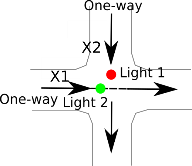
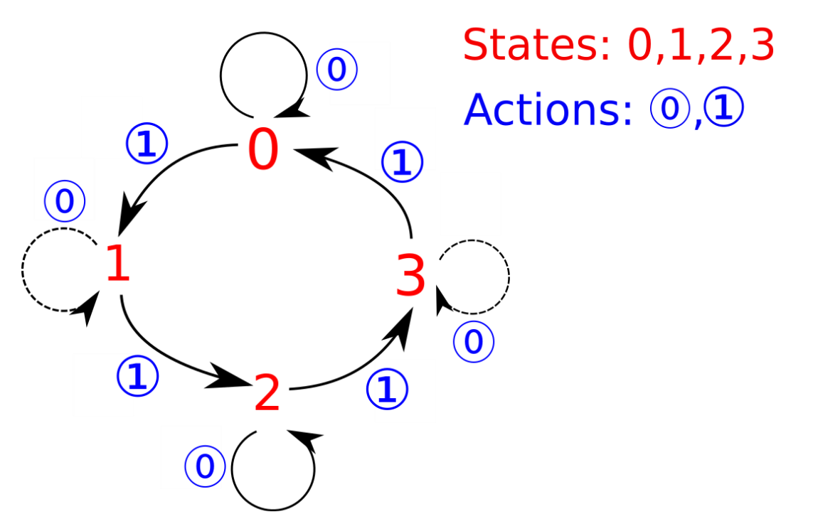
Figure 1: One intersection with two traffic flows (left) where $X_{1}$ and $X_{2}$ are the queue lengths, and the state transition diagram (right).

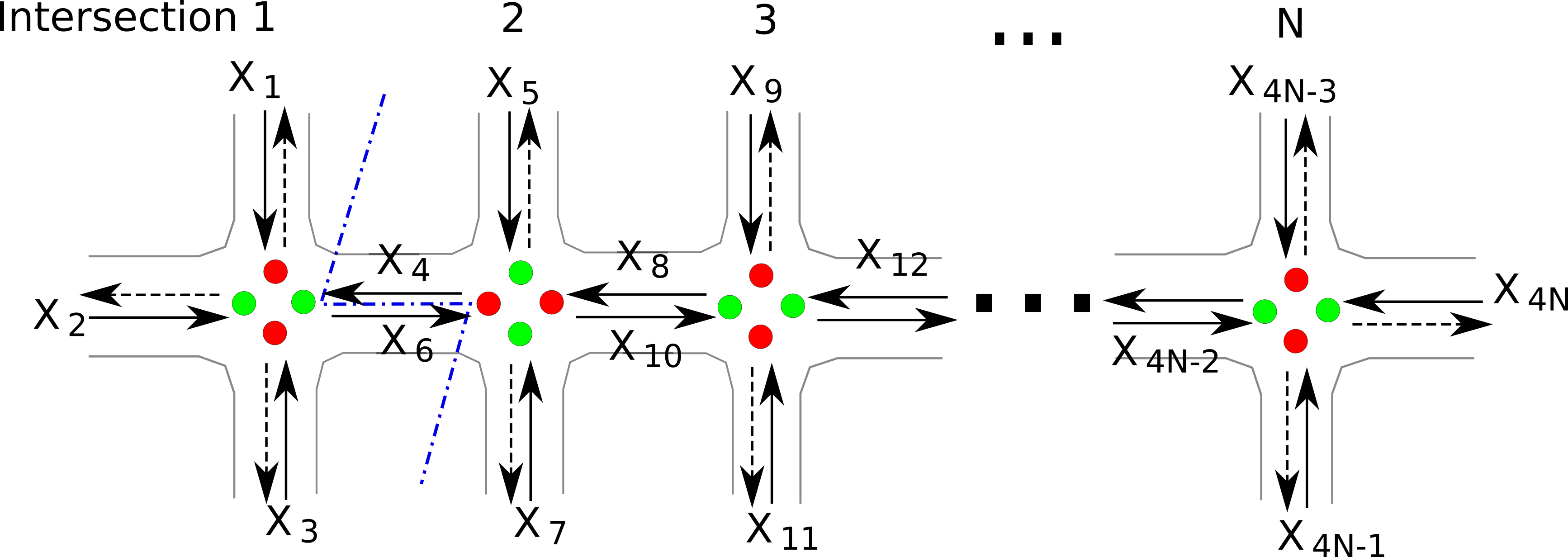
Figure 2: Linear bidirectional road network.

2.1 Single Road Intersection

As mentioned earlier, we start with a single-intersection scenario to facilitate the validation of the DQN algorithms by comparing it with the policy iteration approach. We consider the simplest meaningful setup with two intersecting unidirectional traffic flows as schematically depicted in the left side of Fig. 1. The state $S(t)$ of the system at the beginning of time slot $t$ may be described by the three-tuple $(X_{1}(t),X_{2}(t);Y(t))$, with $X_{i}(t)$ denoting the number of vehicles of traffic flow $i$ waiting to cross the intersection and $Y(t)\in\{0,1,2,3\}$ indicating the configuration of the traffic lights:

• “0”: green light for direction $1$ and hence red light for direction $2$;

• “1”: yellow light for direction $1$ and hence red light for direction $2$;

• “2”: green light for direction $2$ and hence red light for direction $1$;

• “3”: yellow light for direction $2$ and hence red light for direction $1$.

Each configuration $k$ can either simply be continued in the next time slot or must otherwise be switched to the natural subsequent configuration $(k+1)\mod 4$. This is determined by the action $A(t)$ selected at the end of time slot $t$, which is represented by a binary variable as follows: “0” for continue, and “1” for switch:

$$Y(t+1)=(Y(t)+A(t))\mod 4.$$ (1)

These rules give rise to a strictly cyclic control sequence as illustrated in the right side of Fig. 1.

The evolution of the queue state over time is governed by the recursion

$$(X_{1}(t+1),X_{2}(t+1))=(X_{1}(t)+C_{1}(t)-D_{1}(t),X_{2}(t)+C_{2}(t)-D_{2}(t)),$$ (2)

with $C_{i}(t)$ denoting the number of vehicles of traffic flow $i$ appearing at the intersection during time slot $t$ and $D_{i}(t)$ denoting the number of departing vehicles of traffic flow $i$ crossing the intersection during time slot $t$. While not essential for our analysis, we make the simplifying assumption that if one of the two traffic flows is granted the green light, then exactly one waiting vehicle of that traffic flow, if any, will cross the intersection during that time slot, i.e.,

$$D_{1}(t)=\min\{1,X_{1}(t)\}\mbox{ if }Y(t)=0;D_{2}(t)=\min\{1,X_{2}(t)\}\mbox{ if }Y(t)=2;$$ (3)

and $D_{1}(t)=0$ if $Y(t)\neq 0$ and $D_{2}(t)=0$ if $Y(t)\neq 2$.

2.2 Linear Road Topology

To examine the performance and scalability properties of the DQN algorithms in more complex large-scale scenarios, we will consider a linear road topology. Specifically, we investigate a linear network topology with $N$ intersections and bidirectional traffic flows, representing a main artery with cross streets as schematically depicted in Fig 2. We do not account for any traffic flows making left or right turns, but the analysis could easily be generalized to accommodate that. The state $S(t)$ of the system at the beginning of time slot $t$ may be described by a $(5N)$-tuple $(X_{n1}(t),X_{n2}(t),X_{n3}(t),X_{n4}(t);Y_{n}(t))_{n=1,\dots,N}$, with directions $1$ and $2$ corresponding to the east-west direction of the main artery and the north-south direction of the cross streets, and thus

$$Y_{n}(t+1)=(Y_{n}(t)+A_{n}(t))\mod 4,$$ (4)

with $A_{n}(t)$ denoting the action selected for the $n$-th intersection at the end of time slot $t$.

The evolution of the various queue states is governed by the recursion

$$X_{ni}(t+1)=X_{ni}(t)+C_{ni}(t)-D_{ni}(t),$$ (5)

with $C_{ni}(t)$ denoting the number of vehicles in direction $i$ appearing at the $n$ th intersection during time slot $t$ and $D_{ni}(t)$ denoting the number of vehicles crossing the $n$-th intersection in direction $i$ during time slot $t$, $i=1,\dots,4$, $n=1,\dots,N$. While $C_{11}(t)$, $C_{N3}(t)$, and $C_{n2}(t)$, $C_{n4}(t)$, $n=1,\dots,N$, correspond to vehicles approaching the intersection from the external environment, we have $C_{n+1,1}(t+u)=D_{n1}(t)$ and $C_{n3}(t+u)=D_{n+1,3}(t)$, $n=1,\dots,N-1$. This reflects that the vehicles crossing the $n$-th intersection in eastern direction during time slot $t$ appear at the $(n+1)$-th intersection $u$ time slots later; likewise, vehicles passing through the $(n+1)$-th intersection in western direction during time slot $t$ arrive at the $n$-th intersection $u$ time slots later. In this manner, the vehicles that travel along the main artery create highly complex interactions among the various intersections, which present additional challenges in optimizing the control policy.

Note that

$$D_{n1}(t)=\min\{1,X_{n1}(t)\},D_{n3}(t)=\min\{1,X_{n3}(t)\},\mbox{ if }Y_{n}(t)=0,$$ (6)

$D_{n1}(t),D_{n3}(t)=0$ if $Y_{n}(t)\neq 0$, and similarly for $D_{n2}(t)$ and $D_{n4}(t)$ depending on whether $Y_{n}(t)=2$ or not.

2.3 Optimization Goal

We assume that the “congestion cost” in time slot $t$ may be expressed as a function $F(X(t))$ of the queue state, with $X(t)=(X_{1}(t),X_{2}(t))$ in the single-intersection scenario and $X(t)=(X_{n1}(t),X_{n2}(t),X_{n3}(t),X_{n4}(t))_{n=1,\dots,N}$ in the linear topology with $N$ intersections. The goal is to find a dynamic control policy which selects actions over time so as to minimize the long-term expected discounted cost $\mathbb{E}\left[\sum_{t=1}^{\infty}\gamma^{t}F(X(t))\right]$, with $\gamma\in(0,1)$ representing a discount factor.

3 Algorithm Design

We provide a detailed specification of the DQN algorithms for the scenarios of a single intersection or a linear topology with several intersections as described in the previous section.

First of all, let $Q(s,a)$ be the maximum achievable expected discounted reward (or minimum negative congestion cost in our context) under the optimal policy starting from state $s=(X;Y)$ when action $a$ is taken. The $Q(s,a)$ values satisfy the equations

$$Q(s,a)=r(s,a)+\gamma\sum\limits_{s^{\prime}\in\mathcal{S}}p(s,s^{\prime};a)\underset{a^{\prime}\in\mathcal{A}}{\max}Q(s^{\prime},a^{\prime})=r(s,a)+\gamma\mathbb{E}\left[\underset{a^{\prime}\in\mathcal{A}}{\max}Q(s^{\prime},a^{\prime})\right],$$ (7)

with $r(s,a)=F(X)$ denoting the congestion cost in queue state $X$, and $p(s,s^{\prime};a)$ denoting the transition probability from state $s$ to state $s^{\prime}$ when action $a$ is taken. Observe that the values $V(s)=\underset{a^{\prime}\in\mathscr{A}}{\max}Q(s,a^{\prime})$ satisfy the Bellman optimality equations

$$V(s)=\underset{a^{\prime}\in\mathcal{A}}{\max}\{r(s,a)+\gamma\sum\limits_{s^{\prime}\in\mathcal{S}}p(s,s^{\prime};a)V(s^{\prime})\}=\underset{a^{\prime}\in\mathcal{A}}{\max}\{r(s,a)+\gamma\mathbb{E}[V(s^{\prime})]\}.$$ (8)

The system state $S$ serves as the input for both the target network and the evaluate network in the DQN algorithms, with $S=(X_{1},X_{2};Y)$ in the single-intersection scenario and $S=(X_{n1},X_{n2},X_{n3},X_{n4};Y_{n})_{n=1,\dots,N}$ in the linear topology with $N$ intersections. Equation (7) provides the basis for deriving the target Q-values at each time step, while the Q-learning update for the neural network approximator in the $i$-th iteration is calculated based on

$$\text{Loss}(\theta_{i})=\mathbb{E}_{s,a,r,s^{\prime}\sim memory}\bigg{[}\bigg{(}r+\gamma\max\big{(}q\_target(s^{\prime},a^{\prime};\theta^{\prime}_{i})\big{)}-q\_eval(s,a;\theta_{i})\bigg{)}^{2}\bigg{]},$$ (9)

where $r$ is reward (negative cost) in the current step, $s^{\prime}$ and $a^{\prime}$ are the state and action in the next step, $\theta_{i}$ are parameters of the evaluate Q-network in the $i$-th iteration and $\theta^{\prime}_{i}$ are parameters of the target Q-network with delayed update following the evaluate network.

The DQN algorithms sample from and train on data collected in memory. The online samples are stored in memory for further learning. A warm-up period of $k_{0}$ time steps is applied before the learning operations are initiated. The evaluate network is updated with the AdamOptimizer [6] gradient-descent and $\epsilon$-greedy policy, whereas the update of the target network is slightly later.

Based on the above outline, we provide the specification of the DQN algorithm for the single-intersection scenario Fig. 1 and a linear topology with $N$ intersections in Fig. 2. It is worth observing that even in the latter case we adopt a “single-agent” DQN algorithm which has access to the global state of the network, as opposed to the “multiple-agent” method with one agent for each individual intersection as considered in [16, 24]. While the single-agent approach involves a larger state space, it allows more intelligent control and coordination on a global level, which manifests itself for example in the emergence of greenwave patterns as we will demonstrate in the next section.

Algorithm 1 DQN for single intersection or linear road topology with $N$ intersections

  1: Initialize queue and control states: either $X_{1},X_{2}=0;Y=0$ [single intersection] or $X_{n1},X_{n2},X_{n3},X_{n4}=0;Y_{n}=0$ for all $n=1,\dots,N$ [linear topology];

  2: For steps $k=1,\dots,K$ do:

  3:      $s=[X_{1},X_{2};Y]$ [single intersection] or $s=[X_{11},\dots,X_{N4};Y_{1},\dots Y_{N}]$ [linear topology];

  4:     Select action $a$ with $a^{*}=\arg\underset{a\in\mathcal{A}}{\max}~{}q\_{eval}(s;a)$ and $\epsilon$-greedy policy, using eval_net to evaluate the $Q$-value for each action;

  5:     Generate random variables $C_{1}$, $C_{2}$ [single intersection] or $C_{11}$, $C_{N3}$ and $C_{n2}$, $C_{n4}$ for all $n=1,\dots,N$;

  6:      Given $a$, determine new queue and control states $X_{1}^{\prime},X_{2}^{\prime},Y^{\prime}$ according to Eq. (1)-(3) [single intersection] or $X_{11}^{\prime},\dots,X_{N4}^{\prime},Y_{1}^{\prime},\dots,Y_{N}^{\prime}$ according to Eq. (4)-(6) [linear topology];

  7:      $r=-((X_{1}^{\prime})^{2}+(X_{2}^{\prime})^{2})$ [single intersection] or $r=-\sum_{n=1}^{N}\sum_{i=1}^{4}(X_{ni}^{\prime})^{2}$ [linear topology];

  8:      $s^{\prime}=[X_{1}^{\prime},X_{2}^{\prime};Y^{\prime}]$ [single intersection] or $s^{\prime}=[X_{11}^{\prime},\dots,X_{N4}^{\prime};Y_{1}^{\prime},\dots,Y_{N}^{\prime}]$ [linear topology];

  9:     Store transition $[s,a,r,s^{\prime}]$ in memory;

  10:    Perform learning operation if $k>k_{0}$:

  11:          Sample a minibatch of samples from memory;

  12:          Update target network: $\theta^{\prime}_{i}=\theta_{i}$;

  13:          Calculate the target Q-value: $q\_target(s,a)=r+\gamma\underset{a^{\prime}\in\mathcal{A}}{\max}q\_target(s^{\prime},a^{\prime})$;

  14:          Update evaluate network with gradient descent (using AdamOptimizer): $\text{Loss}(\theta_{i})=\mathbb{E}[(q\_target-q\_eval)^{2}]$.

4 Performance Evaluation

We present simulations to evaluate the performance of the DQN algorithm in Alg. 1, and in particular illustrate the emergence of “greenwave” patterns in linear topology networks. Our codes are available at [2].

4.1 Single Road Intersection

As an initial validation benchmark, we first consider a single-intersection scenario as described in Subsection 2.1. The reason for considering this toy scenario is that the state space is sufficiently small for the optimal policy to be computed using the baseline policy iteration approach. We assume the numbers of arriving vehicles of both traffic flows in each time step as represented by the random variables $C_{1}$ and $C_{2}$ to be independent and Bernoulli distributed with parameter $p=1/4$. We use a quadratic congestion cost function $F(X_{1},X_{2})=X_{1}^{2}+X_{2}^{2}$ and a discount factor $\gamma=0.99$.

Inspection of the results in Fig. 3 shows that the DQN policy as obtained using Alg. 1 coincides with the optimal policy with the traditional policy iteration method. In particular, it matches the optimal performance and exhibits a similar threshold structure. This structural property was also reported in [5] for a strongly related two-queue dynamic optimization problem (with switch-over costs rather than switch-over times).

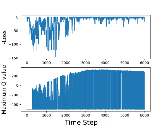
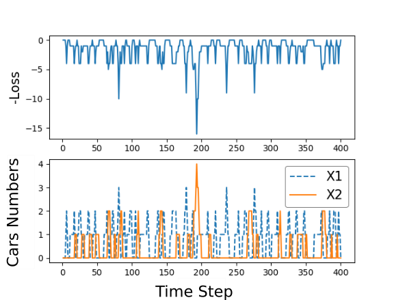
Figure 3: Learning curve for DQN policy (left) and thresholding property of DQN policy (right).

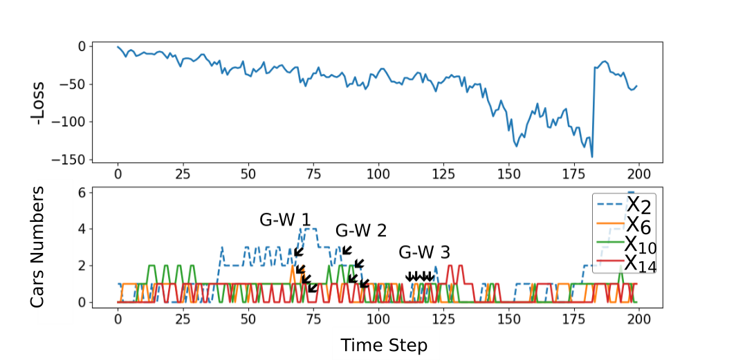
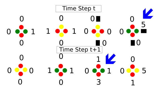
Figure 4: Testing results for the linear network of size $4\times 1$ (left) and Greenwave traffic lights (right). “Greenwave” is abbreviated to be “G-W”. In the right, numbers indicate the number of vehicles waiting on each road. Black rectangles indicate incoming vehicles from peripheral roads.

4.2 Linear Road Topology

We now turn to the scenario in Fig. 2. This is a more challenging scenario which serves to examine the scalability properties of our algorithm and its performance in the presence of highly complex interactions arising from the flow of vehicles along the main east-west arterial road.

Assume the numbers of externally arriving vehicles in eastern and western directions in each time step, represented by the random variables $C_{11}$ and $C_{N3}$, to be independent and Bernoulli distributed with parameter $p_{1}=1/4$. The numbers of arriving vehicles in southern and northern directions on each of the $N$ cross streets in each time step, represented by the random variables $C_{n2}$ and $C_{n4}$, $n=1,\dots,N$, are also independent and Bernoulli distributed with parameter $p_{2}=1/8$. We use a quadratic congestion cost function $F(X)=\sum_{n=1}^{N}\sum_{i=1}^{4}X_{ni}^{2}$ and a discount factor $\gamma=0.99$. In simulations, the evaluate and target networks used in Alg. 1 have both $4$ fully-connected layers of size $200,100,40$ and $2$, respectively. We use ReLu as activation functions and squared difference loss.

The use of a policy iteration approach is computationally infeasible in this case due to the state space explosion, and hence the degree of optimality of our algorithm cannot be assessed in a quantitative manner. Instead we have therefore examined qualitative features to validate the intelligent behavior of our algorithm and evaluate its performance merit. In particular, we observed the emergence of “greenwave” patterns as shown in Fig. 4, even though such structural features are not explicitly prescribed in the optimization process. Specifically, the “greenwave” phenomenon is reflected as consecutive reduction of car numbers in each road. This emergent intelligence confirms the capability of our algorithm to learn favorable structural properties solely from observations.

5 Conclusion

We have explored the scope for Deep Q-Networks (DQN) to optimize real-time traffic light control policies in emerging large-scale Intelligent Transportation Systems. As an initial benchmark, we established that DQN algorithms deliver the optimal performance achieved by the policy iteration approach in a single-intersection scenario. We subsequently evaluated the scalability properties of DQN algorithms in a linear topology with several intersections, and demonstrated the emergence of intelligent behavior such as “greenwave” patterns, confirming their ability to learn desirable structural features.

In future research we intend to investigate locality properties and analyze how these can be exploited in the design of distributed coordination schemes for wide-scale deployment scenarios. It would be interesting to investigate the effectiveness of other RL methods, like Deep Deterministic Policy Gradients (DDPG) used in [25], for transportation systems.

References

- [1] Markov decision processes toolbox: http://www7.inra.fr/mia/t/mdptoolbox/.
- [2] Our codes: http://www.tensorlet.com/.
- [3] Muhammad Alam, Joaquim Ferreira, and José Fonseca. Introduction to intelligent transportation systems. In Intelligent Transportation Systems, pages 1–17. Springer, 2016.
- [4] Andrew Gehret Barto, Steven J Bradtke, and Satinder P Singh. Real-time learning and control using asynchronous dynamic programming. University of Massachusetts at Amherst, Department of Computer and Information Science, 1991.
- [5] Micha Hofri and Keith W Ross. On the optimal control of two queues with server setup times and its analysis. SIAM Journal on Computing, 16(2):399–420, 1987.
- [6] Diederik P Kingma and Jimmy Ba. Adam: A method for stochastic optimization. arXiv preprint arXiv:1412.6980, 2014.
- [7] Stefan Lämmer and Dirk Helbing. Self-control of traffic lights and vehicle flows in urban road networks. Journal of Statistical Mechanics: Theory and Experiment, 4:04019, 2008.
- [8] Stefan Lämmer and Dirk Helbing. Self-stabilizing decentralized signal control of realistic, saturated network traffic. Santa Fe Institute, 2010.
- [9] Yisheng Lv, Yanjie Duan, Wenwen Kang, Zhengxi Li, Fei-Yue Wang, et al. Traffic flow prediction with big data: A deep learning approach. IEEE Trans. Intelligent Transportation Systems, 16(2):865–873, 2015.
- [10] Volodymyr Mnih, Koray Kavukcuoglu, David Silver, Andrei A Rusu, Joel Veness, Marc G Bellemare, Alex Graves, Martin Riedmiller, Andreas K Fidjeland, Georg Ostrovski, et al. Human-level control through deep reinforcement learning. Nature, 518(7540):529, 2015.
- [11] Andrew W Moore and Christopher G Atkeson. Prioritized sweeping: Reinforcement learning with less data and less time. Machine Learning, 13(1):103–130, 1993.
- [12] Simona Onori, Lorenzo Serrao, and Giorgio Rizzoni. Dynamic programming. In Hybrid Electric Vehicles, pages 41–49. Springer, 2016.
- [13] Martin L Puterman. Markov decision processes: discrete stochastic dynamic programming. John Wiley & Sons, 2014.
- [14] Liang Qi, MengChu Zhou, and WenJing Luan. A two-level traffic light control strategy for preventing incident-based urban traffic congestion. IEEE Transactions on Intelligent Transportation Systems, 19(1):13–24, 2018.
- [15] Sheldon M Ross. Introduction to stochastic dynamic programming. Academic Press, 2014.
- [16] Sergey Satunin and Eduard Babkin. A multi-agent approach to intelligent transportation systems modeling with combinatorial auctions. Expert Systems with Applications, 41(15):6622–6633, 2014.
- [17] Rajeshwari Sundar, Santhoshs Hebbar, and Varaprasad Golla. Implementing intelligent traffic control system for congestion control, ambulance clearance, and stolen vehicle detection. IEEE Sensors Journal, 15(2):1109–1113, 2015.
- [18] Richard S Sutton. Learning to predict by the methods of temporal differences. Machine Learning, 3(1):9–44, 1988.
- [19] Elise Van der Pol and Frans A Oliehoek. Coordinated deep reinforcement learners for traffic light control. Proceedings of Learning, Inference and Control of Multi-Agent Systems (at NIPS 2016), 2016.
- [20] Elise van der Pol, Frans A Oliehoek, T Bosse, and B Bredeweg. Video demo: Deep reinforcement learning for coordination in traffic light control. AmsterdamVrije Universiteit, Department of Computer Sciences, 2016.
- [21] MM Vazifeh, P Santi, G Resta, SH Strogatz, and C Ratti. Addressing the minimum fleet problem in on-demand urban mobility. Nature, 557(7706):534, 2018.
- [22] Christopher JCH Watkins and Peter Dayan. Q-learning. Machine Learning, 8(3-4):279–292, 1992.
- [23] Hua Wei, Guanjie Zheng, Huaxiu Yao, and Zhenhui Li. Intellilight: A reinforcement learning approach for intelligent traffic light control. In Proceedings of the 24th ACM SIGKDD International Conference on Knowledge Discovery & Data Mining, pages 2496–2505. ACM, 2018.
- [24] MA Wiering. Multi-agent reinforcement learning for traffic light control. In Proceedings of the Seventeenth International Conference Machine Learning (ICML), pages 1151–1158, 2000.
- [25] Zhuoran Xiong, Xiao-Yang Liu, Shan Zhong, Hongyang Yang, and Anwar Walid. Practical deep reinforcement learning approach for stock trading. NeurIPS Workshop on Challenges and Opportunities for AI in Financial Services: the Impact of Fairness, Explainability, Accuracy, and Privacy, 2018.
- [26] Ming Zhu, Xiao-Yang Liu, Feilong Tang, Meikang Qiu, Ruimin Shen, Wei Wennie Shu, and Min-You Wu. Public vehicles for future urban transportation. IEEE Trans. Intelligent Transportation Systems, 17(12):3344–3353, 2016.
- [27] Ming Zhu, Xiao-Yang Liu, and Xiaodong Wang. Joint transportation and charging scheduling in public vehicle systems—a game theoretic approach. IEEE Transactions on Intelligent Transportation Systems, 19(8):2407–2419, 2018.
- [28] Ming Zhu, Xiao-Yang Liu, and Xiaodong Wang. An online ride-sharing path-planning strategy for public vehicle systems. IEEE Transactions on Intelligent Transportation Systems, 2018.