Entanglement entropy of non-local theories in AdS

Abstract

We investigate the effect of non-locality on entanglement entropy in anti-de Sitter space-time. We compute entanglement entropy of a nonlocal field theory in anti-de Sitter space-time and find several interesting features. We find that area law is followed, but sub-leading terms are affected by non-locality. We also find that the UV finite term is universal. For the massless theory in 3 dimensional AdS we compute it exactly and find the novel feature that it shows oscillatory behavior.

I Introduction

Entanglement entropy is a very useful tool that helps us quantize the correlation between different localized subsystems of a quantum system. For local UV-finite theories entanglement entropy is known to follow an area law Bombelli:1986rw ; Srednicki:1993im . Explicit calculation in $d>2$ can be done for free field theories Casini:2009sr . For field theories with holographic duals, entanglement entropy of a region $A$ can be computed holographically using the quantum corrected Ryu-Takayanagi formula Ryu:2006ef ; Faulkner:2013ana .

$$S_{bdry}(A)=\frac{\text{Area}_{min}}{4G_{N}}+S_{bulk}+\cdots\,.$$ (1)

where Area_min denotes the minimal area surface in the bulk which ends in the boundaries of $A$. The ellipsis refer to higher order corrections in $1/G_{N}$. The last term in the formula is the entanglement entropy in AdS. The entanglement entropy of fields in AdS is therefore an important component of the quantum corrected Ryu-Takayanagi formula and deserves further exploration. So far it has only been calculated for local free fields in AdS Sugishita:2016iel .

Nonlocal field theories present an interesting situation in this context. One would expect that the presence of nonlocal correlations in the theory to manifest itself in entanglement entropy. Indeed it is found that explicit non-locality can have drastic effects on entanglement entropy including modification of area law in some cases Shiba:2013jja ; Karczmarek:2013xxa ; Fischler:2013gsa ; Pang:2014tpa , but not always Nesterov:2010yi ; Nesterov:2010jh ; Solodukhin:2011gn . It is therefore interesting to explore the behaviour of entanglement entropy in field theories which have non-localities.

Nonlocal theories are quite interesting in their own and have been explored in a variety of contexts such as Modesto:2011kw ; Modesto:2017sdr ; Maggiore:2016gpx ; Narain:2017twx ; Narain:2018hxw . Non-local theories have also been explored in the context of black-hole information loss paradox Kajuri:2017jmy ; Kajuri:2018myh .

In this paper we compute entanglement entropy for a particular free non-local field theory. Our action is given by

$$S_{NL}=\int{\rm d}x\sqrt{-g}\biggl{[}\frac{1}{2}(\partial\phi)^{2}+\frac{m^{2}}{2}\phi^{2}-\frac{\lambda^{2}}{2}\phi\frac{1}{-\Box}\phi\biggr{]}\,,$$ (2)

where we refer to $\lambda$ as the non locality scale. It has mass dimensions $[mass]^{2}$. In flat spacetime where it is possible to do a momentum decomposition of fields, it should be noticed that such non-local terms will become important at small energy.

Apart from the general motivations given for computing entanglement entropy in non local field theories, there is a further motivation for this theory. We have shown in a companion paper that these theories admit CFT duals Kajuri:2018wow . This calls for further investigation of these theories in a holographic context. Computation of entanglement entropy of this theory in AdS background would be a step towards a full understanding of the quantum corrected Ryu Takayanagi formula (1) for these theories.

In this paper we consider odd dimensional anti-de Sitter spaces. The entanglement entropy for the theory (2) for generic odd dimensional AdS is computed using the replica trick and the heat kernel method. There are several interesting features. We find that the area law is followed but the sub-leading terms depend on the non-locality scale. We find that there is a UV-finite universal term in entanglement entropy. For massless theories in AdS₃ we explicitly compute it and show that it exhibits oscillatory behaviour. This is a novel feature of nonlocal theories.

The paper is organised as follows. In the section II we study the nonlocal theory (2) in more detail. We calculate the Green function for this theory in flat and AdS space-time in section II.1 and II.2. In the section III we present our computation of entanglement entropy. We summarise our results in the conclusion section IV.

II Non-local scalar field

In this section we consider a local scalar field theory consisting of two coupled fields. This leads to a non-local action once one of the field gets decoupled from the system. Consider the following action for local field theory

$$S=\int{\rm d}x\sqrt{-g}\biggl{[}\frac{1}{2}(\partial\phi)^{2}+\frac{1}{2}(\partial\chi)^{2}+\frac{m^{2}}{2}\phi^{2}-\lambda\phi\chi\biggr{]}\,,$$ (3)

where $\phi$ and $\chi$ are two scalar fields on curved non-dynamical background, $\lambda$ is their coupling strength while $m$ is mass of scalar $\phi$. The equation of motion of two fields give $(-\Box+m^{2})\phi-\lambda\chi=0$ and $-\Box\chi-\lambda\phi=0$. Integrating out $\chi$ from the second equation of motion yields $\chi=\lambda(-\Box)^{-1}\phi$. This when plugged back into the action (3) yields a massive non-local theory for scalar $\phi$ whose action is given by eq. (2). This non-local action has issues of tachyon. In simple case of flat space-time it is noticed that the non-local piece in action reduces to $\phi(-p)(-\lambda^{2}/p^{2})\phi(p)$ (where $\phi(p)$ is the Fourier transform of field $\phi(x)$). This piece correspond to something like tachyonic mass thereby resulting in issues of unitarity and instability of vacuum. Also, in massless case if we write $\phi_{1}=(\phi+\chi)/\sqrt{2}$ and $\phi_{1}=(\phi-\chi)/\sqrt{2}$, then the local action in eq. (3) can be reduced to action of two decoupled free scalar scalar fields $\phi_{1}$ and $\phi_{2}$ of mass $\lambda$ and $-\lambda$ respectively. Immediately we notice the presence of tachyon field $\phi_{2}$. In the massive case things are just more involved, but tachyonic issue remains. In what follows we will therefore consider $\lambda^{2}\to-\lambda^{2}$. This overcomes the issue of tachyons in the non-local theory. Also, it should be mentioned that the resulting non-local theory with $-\lambda^{2}$ can also arise as a low-energy limit of some ultraviolet complete theory in which sense it is an effective theory.

In this section we will study this simple free non-local theory on flat and AdS space-time. In generic space-time the green’s function equation is given by,

$$\biggl{(}-\Box+m^{2}+\frac{\lambda^{2}}{-\Box}\biggr{)}G(x,x^{\prime})=-\frac{i\delta(x-x^{\prime})}{\sqrt{-g}}\,.$$ (4)

II.1 Flat space-time

In this section we study this theory on flat space-time. Understanding the behaviour of theories in flat space-time is important as in curved space-time at ultra-local distances the theory behaves as in flat. This is also required for implementing suitable boundary conditions for the computation of the green’s function.

In flat space-time one can use the momentum space representation to write the propagator. Writing $G(x,x^{\prime})=\int{\rm d}p/(2\pi)\tilde{G}(p)\exp\{ip(x-x^{\prime})\}$, it is seen that

$$G^{\rm NL}_{f}(x,x^{\prime})=-i\int\frac{{\rm d}^{d}p}{(2\pi)^{d}}\biggl{(}p^{2}+m^{2}+\frac{\lambda^{2}}{p^{2}}\biggr{)}^{-1}e^{ip(x-x^{\prime})}$$ (5)

where the subscript in $G_{f}$ implies flat space-time. The integrand can be integrated easily by making use of partial fraction and decomposing it. It can be written in an alternative manner as:

$$\frac{1}{p^{2}+m^{2}+\lambda^{2}/p^{2}}=\frac{p^{2}}{p^{4}+m^{2}p^{2}+\lambda^{2}}=\frac{A}{p^{2}+r_{-}^{2}}+\frac{B}{p^{2}+r_{+}^{2}}\,,$$ (6)

where

$$r_{-}^{2}=\frac{m^{2}-\sqrt{m^{4}-4\lambda^{2}}}{2}\,\hskip 14.22636ptr_{+}^{2}=\frac{m^{2}+\sqrt{m^{4}-4\lambda^{2}}}{2}\,,$$ (7)

while $A=-r_{-}^{2}/(r_{+}^{2}-r_{-}^{2})$ and $B=r_{+}^{2}/(r_{+}^{2}-r_{-}^{2})$. For massless fields ($m^{2}\to 0$) $r_{\pm}^{2}=\pm i\lambda$, $A=1/2$ and $B=1/2$. After the partial fraction each of the piece can be further expressed by using inverse Laplace transform. This allows us to write $\bigl{(}p^{2}+m^{2}+\lambda^{2}/p^{2}\bigr{)}^{-1}$ in inverse Laplace form. Then one can express the flat space-time green’s function in eq. (5) as follows

$$G^{\rm NL}_{f}(x,x^{\prime})=-i\int\frac{{\rm d}^{d}p}{(2\pi)^{d}}\int_{0}^{\infty}{\rm d}s\bigl{[}\cosh(s\beta)-\frac{\alpha}{\beta}\sinh(s\beta)\bigr{]}e^{-s(p^{2}+\alpha)+ip(x-x^{\prime})}\,,$$ (8)

where $\alpha=m^{2}/2$ and $\beta=\sqrt{m^{4}-4\lambda^{2}}/2$. In the integrand one can smoothly take massless limit to obtain green’s function for non-local massless scalar-field. In this massless limit $\alpha\to 0$ while $\beta\to i\lambda$, then the term in square bracket in the integrand still remains real as $\cosh(s\beta)\to\cos(s\lambda)$ and $\sinh(s\beta)\to i\sin(s\lambda)$.

In Eq. (8) one can first evaluate the $p$-integration which is done by completing the square leading to a gaussian type integral. In the process of completing square for $p$, one encounters division by $s$. This implies that the lower limit of $s$-integration should be regularised by imposing a cutoff. One can then perform integration over $p$ easily leading to,

$$G^{\rm NL}_{f}(x,x^{\prime})=\int_{\delta^{2}}^{\infty}{\rm d}s(4\pi s)^{-d/2}e^{-\mu^{2}/4s}\left(Ae^{-sr_{-}^{2}}+Be^{-sr_{+}^{2}}\right)\,,$$ (9)

where $\mu(x,x^{\prime})=\sqrt{(x-x^{\prime})^{2}}$. This is a very subtle definite integral due to the lower limit of integration. This integral can be seen as a sum of two integrals of local theories with masses $r_{-}$ and $r_{+}$ respectively. It is important to understand the singularity structure of this integral carefully as it will be seen to a play an important role later on. As a result we first consider the local field theory which can be obtained from above by taking $\lambda\to 0$ limit. The above integral becomes following

$$G^{\rm L}_{f}(x,x^{\prime})=\int_{\delta^{2}}^{\infty}{\rm d}s(4\pi s)^{-d/2}e^{-\mu^{2}/4s}e^{-sm^{2}}\,.$$ (10)

When $x\neq x^{\prime}$ ($\mu\neq 0$), the integral can be performed exactly in closed form for $\delta=0$. Even otherwise, it is seen that $G^{\rm L}_{f}$ has a taylor series expansion around $\delta=0$. The leading term of which has a singularity which goes as $\sim\mu^{2-d}$. On the other hand it is seen that performing first the small distance expansion and then doing the $s$-integration leads to no short distance singularity in $G_{f}$. This indicates the subtlety associated with the point $(\delta,\mu)=(0,0)$. The standard rule we will follow is to first perform the $s$-integration and then extract the short-distance singularity.

Keeping this in mind eq. (8) is evaluated by first performing the integration over $p$ then integration over $s$. For $m=0$ case the $s$-integral can be performed exactly in closed form in arbitrary dimensions. In four dimensions it acquires a simplified form and is given by,

$$G_{f}(x,x^{\prime})=\frac{\sqrt{i\lambda}K_{1}\left(\sqrt{i\lambda}\mu\right)+\sqrt{-i\lambda}K_{1}\left(\sqrt{-i\lambda}\mu\right)}{8\pi^{2}\mu}\,.$$ (11)

In the case when $m\neq 0$ things are complicated. Here two possibilities arises $m^{4}>4\lambda^{2}$ and $4\lambda^{2}>m^{4}$, where both $m$ and $\lambda$ are positive. In the former case one can take limit $\lambda\to 0$ (locality limit), while in later case one can take the limit $m\to 0$ (massless limit). In the locality limit, $r_{-}^{2}=0$ and $r_{+}^{2}=m^{2}$. In this case $A=0$ while $B=1$ ($\alpha=\beta=m^{2}/2$). In this case one gets the propagator for local massive scalar field which is

$$\left.G^{\rm NL}_{f}(\mu)\right|_{\lambda=0}=(2\pi)^{-d/2}\left(\frac{m}{\mu}\right)^{(d-2)/2}K_{\frac{d}{2}-1}(m\mu)=G_{f}^{L}(\mu)\,,$$ (12)

where $G_{f}^{L}(\mu)$ is the local green’s function of free massive scalar field. For $m\neq 0$ one can still perform integral in closed form. For the massive non-local scalar field in arbitrary space-time dimension this green’s function $G_{f}$ is given by

$$G^{\rm NL}_{f}(\mu)=\frac{(2\pi)^{-d/2}\mu^{1-d/2}}{(r_{+}^{2}-r_{-}^{2})}\times\biggl{[}r_{+}^{d/2+1}K_{\frac{d}{2}-1}\left(r_{+}\mu\right)-r_{-}^{d/2+1}K_{\frac{d}{2}-1}\left(r_{-}\mu\right)\biggr{]}\,,$$ (13)

where $r_{+}$ and $r_{-}$ are stated before. In fact one can express this green’s function as a sum of green’s function for two local massive scalar fields with mass $r_{+}^{2}$ and $r_{-}^{2}$ and, coefficient $A$ and $B$ respectively. This is expected and is clear from eq. (9). As a result one can also write $G_{f}^{\rm NL}$ as

$$G^{\rm NL}_{f}(\mu)=\left.AG_{f}^{L}(\mu)\right|_{r_{-}}+\left.BG_{f}^{L}(\mu)\right|_{r_{+}}\,.$$ (14)

This will also be useful in fixing the appropriate boundary conditions for the green’s function on AdS. One can do a short distance expansion of the flat space-time green’s function to isolate the singular behaviour of the propagator. In four dimensions the two singular contributions are:

$$G_{f}^{\rm sing}=\frac{1}{4\pi^{2}\mu^{2}}+\frac{m^{2}}{8\pi^{2}}\log(\mu)+\cdots\,,$$ (15)

where $\mu=\mu(x,x^{\prime})$. These are singular behaviour in four dimension at short distances. This will be true in other even dimensions where the leading singularity will be $\sim\mu^{2-d}$. In even and odd dimensions we have the short distance singularity structure as

$$\left.G_{f}^{\rm sing}\right|_{\rm d=even}=a_{0}\mu^{2-d}+a_{1}\mu^{4-d}+\cdots a_{L}\log\mu\,,$$

$$\left.G_{f}^{\rm sing}\right|_{\rm d=odd}=a_{0}\mu^{2-d}+a_{1}\mu^{4-d}+\cdots+\frac{a_{L}}{\mu}\,.$$ (16)

The $\log\mu$ contribution in even dimensions is also singular though in infrared limit ($\mu\to\infty$) it has a well-defined behaviour. In massive theories one also has an inbuilt infrared cutoff $\Lambda_{\rm IR}\sim 1/m$, which truncates the IR modes of the theory. Then it is noticed that the $\log\mu$ approaches $\log\Lambda_{\rm IR}=-\log m$ in IR. This implies that the $\log$ contribution in $G_{f}\sim-m^{2}\log m$ which has a smooth massless limit.

II.2 Anti-DeSitter (AdS)

In this section we will investigate the theory eq. (2) in Euclidean AdS (EAdS) background. The $n$-dimensional EAdS space-time $\mathbb{H}^{n}$ can be identified with the real upper-sheeted hyperboloid in $(d+1)$ Minkowski space-time $M_{d+1}$: $X_{d}=\{x\in\mathbb{R}^{d+1},x_{1}^{2}+\cdots+x_{d}^{2}-x_{d+1}^{2}=-H^{-2}\}$, where $H$ is related to EAdS length. If the two points are denoted by $x$ and $x^{\prime}$, the length of geodesic connecting them is $\mu(x,x^{\prime})$. It is useful to introduce a quantity $z(x,x^{\prime})=\cosh^{2}(H\mu/2)$. For time-like distances $\mu^{2}<0$ which corresponds to $0\leq z<1$, while space-like separation $0<\mu^{2}<\infty$ corresponds to $1<z<\infty$. $z=1$ is the light-like separation. On AdS background the Green’s function will be entirely a function of $\mu$ (or $z(x,x^{\prime})$). This allows one to compute green’s function exactly by solving linear differential equations.

In the case of non-local theory, the green’s function equation is given in eq. (4). Before we solve for $G(x,x^{\prime})$ on AdS, we first note the following important identities on curved space-time.

$$-[\Box^{2}-m^{2}\Box+\lambda^{2}]^{-1}\Box=A(-\Box+r_{-}^{2})^{-1}+B(-\Box+r_{+}^{2})^{-1}\,,$$ (17)

where $A$, $B$, $r_{-}^{2}$ and $r_{+}^{2}$ have the same values as in flat space-time. If we multiply both sides by operator

$$[\Box^{2}-m^{2}\Box+\lambda^{2}]=(-\Box+r_{-}^{2})(-\Box+r_{+}^{2})\,,$$ (18)

then we clearly note that it is identically satisfied. It is this identify which allows us to compute the green’s function of the non-local theory in anti-deSitter space-time. This means that the full green’s function for non-local theory $G_{\rm NL}(x,x^{\prime})$ is a sum of two green’s function

$$G_{\rm NL}(x,x^{\prime})=AG_{-}(x,x^{\prime})+BG_{+}(x,x^{\prime})\,,$$ (19)

where

$$(-\Box+r_{-}^{2})G_{-}(x,x^{\prime})=0\,,\hskip 14.22636pt(-\Box+r_{+}^{2})G_{+}(x,x^{\prime})=0\,$$ (20)

are the two green’s function on AdS which are determined by requiring that the short distance singularity of AdS propagator to match with the singular behaviour of the flat space-time propagator. This is just gives the usual AdS propagator of the free local massive scalar field which is well known in literature Avis:1977yn ; Allen:1985wd ; Burgess:1984ti ; Caldarelli:1998wk . For example, for local massive scalar field on AdS we have $(-\Box+m^{2})G(x,x^{\prime})=0$ as Green’s function equation. Then $G(x,x^{\prime})$ follows

$$z(1-z)G^{\prime\prime}+\left[c-(a+b+1)z\right]G^{\prime}-abG=0\,,$$ (21)

where $a=\bigl{[}d-1+\bigl{(}(d-1)^{2}+4m^{2}/H^{2}\bigr{)}^{1/2}\bigr{]}/2$, $b=\bigl{[}d-1-\bigl{(}(d-1)^{2}+4m^{2}/H^{2}\bigr{)}^{1/2}\bigr{]}/2$ and $c=d/2$. This Hyper-geometric differential equation has two linearly independent solution: $z^{-a}{}_{2}F_{1}(a,a-c+1,a-b+1;z^{-1})$ and $z^{-b}{}_{2}F_{1}(b,b-c+1,b-a+1;z^{-1})$ Avis:1977yn ; Allen:1985wd ; Burgess:1984ti ; Caldarelli:1998wk ; Gubser:2002zh . As $a>0$ and $b<0$, therefore the former solution fall off at boundary of AdS while the later doesn’t. This allow one to pick the former. By requiring the short distance singularity of AdS propagator to match with the singular behaviour of the flat space-time propagator one concludes that $G(z)=q\times z^{-a}{}_{2}F_{1}(a,a-c+1,a-b+1;z^{-1})$. The coefficient $q$ is fixed by requiring that the strength of singularity of AdS propagator matches with the strength of singularity in flat space-time. This gives,

$$q=\frac{(4\pi)^{(1-d)/2}2^{-(a-b+1)}H^{d-2}\Gamma(a)}{\Gamma(a-c+3/2)}\,.$$ (22)

Using this one can write the Green’s function $G_{NL}$ for non-local scalar on AdS to be

$$G_{\rm NL}(z)=Aq_{-}\,z^{-a_{-}}{}_{2}F_{1}(a_{-},a_{-}-c_{-}+1,a_{-}-b_{-}+1;z^{-1})$$

$$+Bq_{+}\,z^{-a_{+}}{}_{2}F_{1}(a_{+},a_{+}-c_{+}+1,a_{+}-b_{+}+1;z^{-1})\,,$$ (23)

where the coefficients $q_{-}$ and $q_{+}$ are determined from eq. (22) with mass replaced by $r_{-}$ and $r_{+}$ respectively, while $A$ and $B$ are same as previous mentioned. The parameters of the hyper-geometric functions are given by

$$a_{-}=\frac{1}{2}\left(d-1+\sqrt{(d-1)^{2}+\frac{4r_{-}^{2}}{H^{2}}}\right)\,,\hskip 5.69054ptb_{-}=\frac{1}{2}\left(d-1-\sqrt{(d-1)^{2}+\frac{4r_{-}^{2}}{H^{2}}}\right)\,,$$ (24)

$$a_{+}=\frac{1}{2}\left(d-1+\sqrt{(d-1)^{2}+\frac{4r_{+}^{2}}{H^{2}}}\right)\,,\hskip 5.69054ptb_{+}=\frac{1}{2}\left(d-1-\sqrt{(d-1)^{2}+\frac{4r_{+}^{2}}{H^{2}}}\right)\,,$$

and $c_{-}=c_{+}=d/2$. The parameters $q_{-}$ and $q_{+}$ are given by,

$$q_{-}=\frac{2^{-(a_{-}-b_{-}+1)}H^{d-2}\Gamma(a_{-})}{(4\pi)^{(d-1)/2}\Gamma(a_{-}-c_{-}+3/2)}\,,\hskip 8.53581ptq_{+}=\frac{2^{-(a_{+}-b_{+}+1)}H^{d-2}\Gamma(a_{+})}{(4\pi)^{(d-1)/2}\Gamma(a_{+}-c_{+}+3/2)}\,.$$ (25)

The green’s function is analytic in $\lambda$. By taking $\lambda\to i\lambda$ one obtains green’s function for theory with tachyons. The green’s function remains well-defined even when this transformation is done. The massless limit can be smoothly taken on AdS irrespective of non-locality. In the massless limit $r_{+}^{2}\to i\lambda$ while $r_{-}^{2}\to-i\lambda$, while $A\to 1/2$ and $B\to 1/2$. Correspondingly the parameters of hyper-geometric functions can be obtained (see Narain:2018rif for non-local green’s function in deSitter).

In Figure 1 we plot this green’s function for various values of $\lambda_{s}$ for massless theory. It is seen that non-locality starts to have effect on the propagator at short distances.

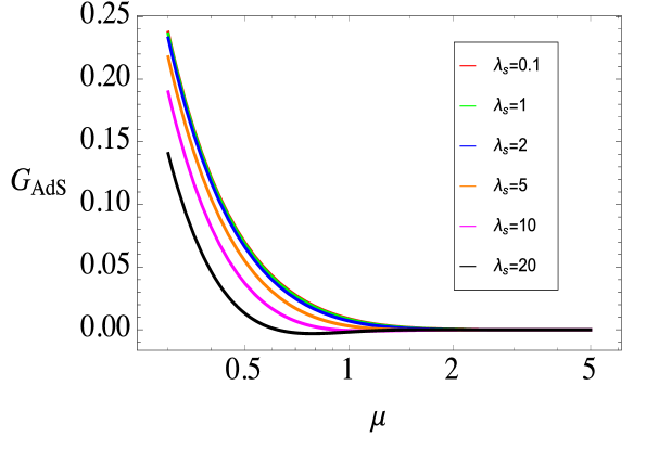
Figure 1: The Green’s function of massless non-local scalar field in four space-time dimensions. The propagator is plotted for various strength of non-locality $\lambda$ against the for space-like separation $\mu(x,x^{\prime})$.

For the case of non-zero mass, the propagator has one more parameter, however structure remains same. Here we have three cases (as in flat space-time): $m^{2}<2\lambda$, $m^{2}=2\lambda$ and $m^{2}>2\lambda$. In each case the propagator is real for space-like separation. It is worthwhile to plot the propagator for fixed value of $\lambda_{s}$ and for decreasing mass. It is seen that as $m\to 0$, the massive propagator smoothly approaches the massless non-local propagator. In figure 2 we plot this scenario.

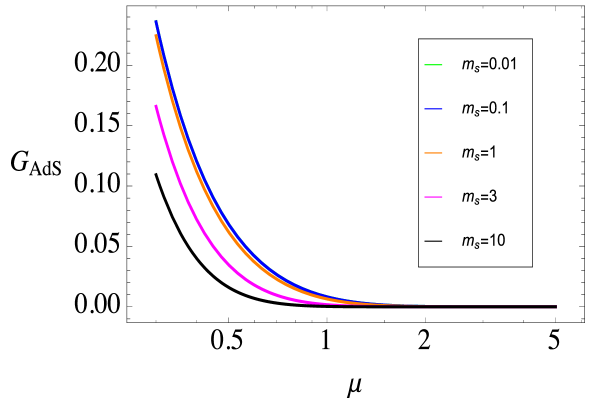
Figure 2: The Green’s function of massive non-local scalar field in four space-time dimensions. The propagator is plotted for various mass $m_{s}$ and for fixed $\lambda_{s}=1$, against the for space-like separation $\mu(x,x^{\prime})$.

The case of equality is interesting as then the propagator depends only on one parameter. Physically it implies that the two length scales are comparable. In this case the non-locality scale is coupled with the mass, so $m\to 0$ implies $\lambda\to 0$ simultaneously. The infrared limit of mass going to zero is well-defined and smooth. In this limit the non-local green’s function is independent of any parameters in the theory (depending only on $H$). It is given by,

$$\left.G_{\rm NL}\right|_{m^{2}=2\lambda}=\frac{H^{2}\left[2z+2(z-1)z\log\left(\frac{z-1}{z}\right)-1\right]}{16\pi^{2}(z-1)z}\,.$$ (26)

On doing the short distance expansion $\mu\to 0$ it is noticed that the leading singular behaviour of $G_{\rm AdS}(\mu)$ is exactly the same as in flat space-time, which is expected due to boundary conditions. Beside this there is next-to-leading singular piece in four space-time dimensions. This term is $\log$-divergent and is given by $((2H^{2}+m^{2})/8\pi^{2})\log\mu$. Compared to flat space-time, here there is extra contribution from $H$. Again, this term doesn’t depend on the non-locality strength $\lambda$. This again is not problematic in IR as argued in flat space-time. Beside this there will also be terms like $\mu\log\mu$ which will appear in higher-order expansion of the green’s function. Terms like these are not UV-singular in the short distance limit. It is noted that in short-distance expansion one can arrange the various terms as the following series

$$G_{\rm NL}=-\frac{\pi^{1-d/2}2^{-d}\csc(d\pi/2)}{H^{d-2}\Gamma(2-d/2)}\frac{1}{(z-1)^{d/2-1}}+\frac{E_{2}}{(z-1)^{d/2-2}}+\cdots+E_{0}\,,$$ (27)

where $E_{0}$ is a constant piece in $z$ depending on mass $m$, non-locality strength $\lambda$, $H$ and dimension $d$. This is a kind of universal piece as it is present in the expression of $G_{\rm NL}$ for all $z$. This term is given by,

$$E_{0}=\frac{H^{d-2}\pi^{1-d/2}\csc(d\pi/2)}{2^{d}\Gamma(d/2)(r_{+}^{2}-r_{-}^{2})}\left[\frac{r_{+}^{2}\Gamma(a_{+})}{\Gamma(1-b_{+})}-\frac{r_{-}^{2}\Gamma(a_{-})}{\Gamma(1-b_{-})}\right]\,.$$ (28)

III Entanglement entropy

In this section we compute the entanglement entropy (EE) in the AdS background using the replica trick Callan:1994py ; Holzhey:1994we ; Calabrese:2004eu ; Calabrese:2009qy . Replica trick is covariant formulation of the computation of either EE or Renyi entropy via usage of effective action of the theory which is computed on a background with conical defect.

The actual starting point is density matrix $\rho$. Any space can be divided by a surface $\Sigma$ in to two parts: $A$ and $\bar{A}$. The field modes resides on both the sides of the boundary surface $\Sigma$ (the projection of this on boundary is $B$). This has been depicted in the figure 3.

Figure 3: Minimal surface corresponding to region $B$ in the boundary. The $z$-direction denotes the bulk while the $x$ represent the spatial co-ordinate on boundary. The region surrounded by $B$ is $\Sigma$ and is denoted by $A$.

This leads to a Hilbert space factorisation: $H=H_{A}\otimes H_{\bar{A}}$. Then tracing out degree of freedom on $\bar{A}$ result in reduced density matrix: $\rho_{A}={\rm Tr}[\ket{\psi}\bra{\psi}]$, where $\bar{\psi}$ is a ground state. The entanglement entropy $S_{A}$ will be defined as: $S_{A}=-{\rm Tr}(\rho_{A}\log\rho_{A})$. In order to compute EE for field theoretic systems one has to make use of replica trick, which make use of path-integral formalism. In this one start by expressing the density matrix in the path-integral form. Following Ryu:2006ef we first define a vacuum state of QFT by path-integral over half of total Euclidean space $\tau\leq 0$, in such a manner that the quantum field takes a fixed boundary condition $\psi(\tau=0,x)=\psi_{0}(x)$. Then we have

$$\Psi[\psi_{0}(x)]=\int_{\psi(\tau=0,x)=\psi_{0}(x)}{\cal D}\psi\exp(-I)\,,$$ (29)

where $I$ is the euclidean action of the field $\psi$ and $\Psi$ is a functional of boundary $\psi_{0}$. The direction of $x$ is orthogonal to boundary $\Sigma$. The surface defined by $x=0$ , $\tau=0$ naturally divides the surface $\Sigma$ in two parts: $x>0$ and $x<0$. Correspondingly the boundary data gets separated as $\psi_{\pm}(x)=\psi_{0}(x)$ for $x>0$ and $x<0$ respectively. Tracing out over $\psi_{-}$ results in a reduced density matrix

$$\rho(\psi_{+}^{1},\psi_{+}^{2})=\int{\cal D}\psi_{-}\Psi(\psi_{+}^{1},\psi_{-})\Psi(\psi_{+}^{2},\psi_{-})\,,$$ (30)

where the path-integral goes over whole euclidean space-time except the cut at $\tau=0$, $x>0$, while the field $\psi(A)$ takes the value $\psi^{2}_{+}$ above the cut and $\psi^{1}_{+}$ below the cut. The quantity ${\rm Tr}\rho^{n}$ is then defined over $n$-sheeted copy of the cut space-time, where appropriate analytic gluing is done when passing from one sheet to another. This quantity is given by,

$${\rm Tr}\rho^{n}=\frac{Z_{n}}{Z_{1}^{n}}\,,$$ (31)

where $Z_{n}$ is the path-integral over the $n$-sheeted covering space ${\cal M}^{n}$ which is obtained by analytically sewing $n$-copies of the original euclidean manifold ${\cal M}$ along the cut. The EE and Renyi entropy are correspondingly given by

$$S_{EE}=\lim_{n\to 1}(n\partial_{n}-1)W_{n}\,,\hskip 14.22636ptS_{n}=\lim_{n\to 1}\frac{W_{n}-nW_{1}}{n-1}\,,$$ (32)

where $W_{n}=-\log Z_{n}$ is the effective action on ${\cal M}^{n}$ while $W_{1}=\log Z_{1}$ is the usual effective action on ${\cal M}$.

The effective action $W_{1}$ (where $1$ indicates the EA has been computed on the single-copy of manifold ${\cal M}$) for field theory can be computed using the standard field theory methods in flat space-time. On curved space there are limitations as the usual Feynman perturbation theory cannot be directly extended. However, one can still perform some computations on maximally symmetric background or one-loop approximation. In the later case, the effective action $W_{1}$ to one-loop can be expressed using the heat-kernel of the Hessian of the theory on the curved background.

$$W=-\frac{1}{2}\int_{0}^{\infty}\frac{{\rm d}s}{s}{\rm Tr}K(x,x;s)=-\lim_{x\to x^{\prime}}\frac{1}{2}\int_{0}^{\infty}\frac{{\rm d}s}{s}{\rm Tr}\bra{x}\exp(-s\triangle)\ket{x^{\prime}}\,,$$ (33)

where $K(x,x^{\prime};s)$ is the heat-kernel of the operator $\triangle$, while $x$ and $x^{\prime}$ are two space-time points and ${\rm Tr}$ is over all Lorentz and space-time index. The lower limit of the $s$-integral is not well-defined and leads to UV divergences which also arise due to co-incident limit. In fact the integrand is singular at $s=0$. One has to impose a cutoff which correspond to imposing an ultraviolet cutoff in theory. This singles out precisely the divergent part of the above integral leaving behind a UV-finite piece.

In the replica-method, the entropy is computed by first obtaining the effective action on the background of $n$-manifold (${\cal M}^{n}$). This can be computed by exploiting the known results of heat-kernel of operator on background of cone Dowker:1977zj ; Dowker:1987mn ; Solodukhin:2011gn ; Fursaev:1994in and making use of Sommerfeld formula Sommerfeld:1897 which expresses heat-kernel modification on the such a manifold with conical singularity as

$$K_{n}(\phi,\phi^{\prime};s)=K_{1}(\phi,\phi^{\prime};s)+\frac{i}{4\pi n}\int_{\Gamma}{\rm d}\omega\cot\left(\frac{\omega}{2n}\right)K_{1}(\phi-\phi^{\prime}+\omega;s)\,,$$ (34)

where $\phi$ is the angle and other co-ordinates have been skipped, the contour $\Gamma$ consists of two lines: one goes from $(-\pi+i\infty)$ to $(-\pi-i\infty)$ intersecting the real axis between the poles $-2\pi n$ and 0 of $\cot(\omega/2n)$, and another goes from $(\pi-i\infty)$ to $(\pi+i\infty)$ intersecting the real axis between the poles 0 and $2\pi n$. For $n=1$ the integrand is $2\pi$-periodic and the contribution from the two vertical lines cancel each other.

This modification of heat-kernel on ${\cal M}^{n}$ gets reflected on the computation of one-loop effective action and the green’s function on ${\cal M}^{n}$, and allows to do the computation of the entropy via replica trick. In the case of AdS one then has to go to co-ordinate system where it is possible to successfully implement the procedure of having $n$-copies of manifold where gluing is done analytically to have construct ${\cal M}^{n}$. The maximally symmetric EAdS can be represented as an embedding of surface

$$x_{1}^{2}+\cdots+x_{d}^{2}-x_{d+1}^{2}=-H^{-2}$$ (35)

in $\mathbb{R}^{1,d}$ with metric

$${\rm d}s^{2}={\rm d}x_{1}^{2}+\cdots+{\rm d}x_{d}^{2}-{\rm d}x_{d+1}^{2}\,.$$ (36)

Under the transformation $x_{d+1}+x_{d}=z^{-1}H^{-2}$, $x_{a}=(Hz)^{-1}y_{a}$, the induced metric on the above hyperboloid then becomes a standard $AdS_{d}$ metric:

$${\rm d}s^{2}=(Hz)^{-2}({\rm d}z^{2}+\eta_{ab}{\rm d}y^{a}{\rm d}y^{b})\,.$$ (37)

If one polar transforms $z$ and $y$, implying $z=r\sin\theta$ and $y=r\cos\theta$, then the entangling surface $\Sigma$ is given by $r=r_{0}$ and $t_{E}=0$. $EAdS_{d}$ has another useful foliation given by:

$$x_{d+1}=\sqrt{\rho^{2}+L^{2}}\cosh u\,,\hskip 5.69054ptx_{1}=\rho\sin(\tau/L),\hskip 5.69054ptx_{d}=\rho\cosh(\tau/L)\,,$$

$$x_{2}=\sqrt{\rho^{2}+L^{2}}\sinh(u)\cos(\phi_{1})\,,\hskip 5.69054ptx_{3}=\sqrt{\rho^{2}+L^{2}}\sinh(u)\sin(\phi_{1})\cos(\phi_{2})\,,\hskip 5.69054pt\cdots,$$

$$x_{d-2}=\sqrt{\rho^{2}+L^{2}}\sinh(u)\sin(\phi_{1})\sin(\phi_{2})\cdots\sin(\phi_{d-2})\,,$$ (38)

where $L=H^{-1}$ Casini:2011kv ; Hung:2014npa . This transformation expresses the EAdS space-time as a Euclidean topological black-hole whose horizon is hyperbolic space $H^{d-2}$. This metric is given by,

$${\rm d}s^{2}=\frac{{\rm d}\rho^{2}}{1+H^{2}\rho^{2}}+H^{2}\rho^{2}{\rm d}\tau_{E}^{2}+(H^{-2}+\rho^{2})({\rm d}v^{2}+\sinh^{2}v\,{\rm d}\Omega_{d-3}^{2})\,.$$ (39)

where the horizon occurs at $\rho=0$ having a uniform negative curvature. This topological black hole has a horizon temperature $T=H/(2\pi)$. The entangling surface $\Sigma$ correspond to this horizon at $\tau_{E}=0$. We represent the area of this entangling surface by ${\cal A}(\Sigma)$ which has been computed in Casini:2011kv ; Sugishita:2016iel . For the $n$-copies of this manifold, the covering space ${\cal M}^{n}$ has the period $\tau_{E}\sim\tau_{E}+2n\pi/H$. The partition function $Z_{n}$ acquires a thermal nature with temperature $H/(2n\pi)$.

On the AdS geometry, which is maximally symmetric, one can compute the heat-kernel $K_{1}(x,x^{\prime};s)$ exactly Camporesi:1990wm , using which one can compute the effective action by making use of the relation eq. (33). This can then be used to compute the entropy. The effective action involves trace of the heat-kernel. Using the above co-ordinate system eq. (39) the trace of the heat-kernel is given by,

$${\rm Tr}K_{n}(s)=H^{3-d}\int_{0}^{2\pi n/H}{\rm d}\tau_{E}\int_{H^{d-2}}{\rm d}V_{d-2}\int_{0}^{\infty}{\rm d}\rho\,\rho(1+H^{2}\rho^{2})^{\frac{d-3}{2}}K_{n}(x,x;s)$$

$$=n{\rm Tr}K_{1}(s)+\frac{i}{2}\frac{{\cal A}(\Sigma)}{H^{d-2}}\int_{0}^{\infty}{\rm d}\rho\rho(1+H^{2}\rho^{2})^{\frac{d-3}{2}}\int_{\Gamma}{\rm d}\omega\cot\left(\frac{\omega}{2n}\right)K_{1}(\mu;s)\,,$$ (40)

where

$$z(x,x^{\prime})=\cosh^{2}\left(\frac{H\mu}{2}\right)=1+(H\rho)^{2}\sin^{2}(H(\tau_{E}-\tau_{E}^{\prime}))=1+(H\rho)^{2}\sin^{2}(\omega/2)$$ (41)

is the EAdS invariant quantity for the points two $x$ and $x^{\prime}$ which differ only in $\tau_{E}$-direction for the EAdS metric stated in eq. (39), while $\mu(x,x^{\prime})$ is the geodesic distance between $x$ and $x^{\prime}$. The expression for the trace of heat-kernel immediately give us the expression for the effective action on ${\cal M}^{n}$ using eq. (33) which can be used to compute entropy. The expression of the effective action is given by,

$$W_{n}=nW_{1}-\frac{i}{2}\frac{{\cal A}(\Sigma)}{H^{d-2}}\int_{\delta^{2}}^{\infty}\frac{{\rm d}s}{s}\int_{0}^{\infty}{\rm d}\rho\rho(1+H^{2}\rho^{2})^{\frac{d-3}{2}}\int_{\Gamma}{\rm d}\omega\cot\left(\frac{\omega}{2n}\right)K_{1}(\mu;s)\,.$$ (42)

The EE (or Renyi) can be computed following eq. (32) which is then given by,

$$S_{\rm EE}=\lim_{n\to 1}-\frac{-i{\cal A}(\Sigma)}{2H^{d-2}}(n\partial_{n}-1)F(n)\,,$$ (43)

$$S_{\rm Renyi}=\lim_{n\to 1}-\frac{i}{2(n-1)}\frac{{\cal A}(\Sigma)}{H^{d-2}}F(n)\,,$$ (44)

where

$$F(n)=\int_{\delta^{2}}^{\infty}\frac{{\rm d}s}{s}\int_{0}^{\infty}{\rm d}\rho\rho(1+H^{2}\rho^{2})^{\frac{d-3}{2}}\int_{\Gamma}{\rm d}\omega\cot\left(\frac{\omega}{2n}\right)K_{1}(\mu;s)\,,$$ (45)

$\cosh^{2}\left(\frac{H\mu}{2}\right)=1+(H\rho)^{2}\sin^{2}(\omega/2)$ and $K_{1}(\mu;s)$ is the EAdS heat-kernel on manifold ${\cal M}$ Camporesi:1990wm . This is the exact expression for the EE and Renyi entropy, and it goes as the area of the surface $\Sigma$ which is denoted above by ${\cal A}(\Sigma)$.

The integral stated in eq. (45) however is not easy to compute. It consists of three integrals: one over $\rho$ which can be traded to integral over $\mu$ using the relation $\cosh^{2}\left(\frac{H\mu}{2}\right)=1+(H\rho)^{2}\sin^{2}(\omega/2)$, the second is a contour integral over $\omega$ for contour $\Gamma$ while the last integral is over $s$. In the former one can do transformation of variables from $\rho$ to $\mu$. This leads to following expression for $F(n)$.

$$F(n)=\frac{1}{4H}\int_{\delta^{2}}^{\infty}\frac{{\rm d}s}{s}\int_{\Gamma}{\rm d}\omega\frac{\cot\left(\omega/2n\right)}{\sin^{2}(\omega/2)}\int_{0}^{\infty}{\rm d}\mu\sinh(H\mu)\left[1+\frac{\sinh^{2}\left(H\mu/2\right)}{\sin^{2}\left(\omega/2\right)}\right]^{(d-3)/2}K_{1}^{d}(\mu;s)\,,$$ (46)

where $K_{1}^{d}(\mu;s)$ is the heat-kernel on the AdS metric which is well known from the literature Camporesi:1990wm . This integral is not easy to perform in arbitrary dimensions, however in odd dimensions the expression in square brackets becomes a polynomial in $\sinh^{2}(H\mu/2)$ when expanded. This offers some simplicity in obtaining expression for entropy in odd dimensions.

III.1 Non-local heat-kernel and effective action

The quantity that enters the computation of the entropy is the effective action. In this sun-section we will compute the effective action of the theory considered here by making use of the heat-kernel on the AdS. For the free non-local theory considered in eq. (2) (with the negative $-\lambda^{2}$) the effective action is given by,

$$W =-\log Z=\frac{1}{2}\log\det\left(-\Box+m^{2}+\frac{\lambda^{2}}{-\Box}\right)=\frac{1}{2}\log\det\left[(-\Box)^{-1}\left(\Box^{2}-m^{2}\Box+\lambda^{2}\right)\right]\,,$$

$$=-\frac{1}{2}\log\det(-\Box)+\frac{1}{2}\log\det(-\Box+r_{-}^{2})+\frac{1}{2}\log\det(-\Box+r_{+}^{2})\,,$$ (47)

where in obtaining last line we have used eq. (18) and, $r_{-}^{2}$ and $r_{+}^{2}$ are given in eq. (7) respectively. Each of the piece in the last line of eq. (III.1) can be expressed in terms of heat-kernel of $\Box$-operator on AdS which gives the following expression for the effective action of our theory

$$W_{1}=\lim_{x\to x^{\prime}}\frac{1}{2}\int_{\delta^{2}}^{\infty}\left(-\frac{{\rm d}s}{s}\right)\left(e^{-sr_{+}^{2}}+e^{-sr_{-}^{2}}-1\right){\rm Tr}K_{0}(x,x^{\prime};s)\,,$$ (48)

where $K_{0}(x,x^{\prime};s)=\bra{x}e^{-s(-\Box)}\ket{x^{\prime}}$ is the heat-kernel of the $\Box$. The eq. (48) tell us that $K_{1}$ appearing in eq. (46) is given by

$$K_{1}(x,x^{\prime};s)=\left(e^{-sr_{+}^{2}}+e^{-sr_{-}^{2}}-1\right)K_{0}(x,x^{\prime};s)\,.$$ (49)

In the case when non-locality strength goes to zero ($\lambda\to 0$) one recovers the heat-kernel of the local massive scalar field operator as $r_{-}^{2}\to 0$. The heat-kernel $K_{0}$ on AdS background is known in closed form exactly Camporesi:1990wm and is different in odd and even dimensions. For the AdS geometry it is given by,

$$K_{0}^{\rm odd} =\left(\frac{-1}{2\pi}\right)^{\frac{d-1}{2}}(4\pi s)^{-1/2}\left[\frac{H}{\sinh(H\mu)}\frac{\partial}{\partial\mu}\right]^{\frac{d-1}{2}}\exp\left[-\frac{\mu^{2}}{4s}-\frac{(d-1)^{2}H^{2}s}{4}\right]\,,$$ (50)

$$K_{0}^{\rm even} =\left(\frac{-1}{2\pi}\right)^{\frac{d-2}{2}}\frac{\sqrt{2}e^{-(d-1)^{2}H^{2}s/4}}{(4\pi s)^{3/2}}\left[\frac{H}{\sinh(H\mu)}\frac{\partial}{\partial\mu}\right]^{\frac{d-2}{2}}\int_{H\mu}^{\infty}{\rm d}\mu^{\prime}\frac{H^{2}\mu^{\prime}e^{-\mu^{\prime 2}/4s}}{\sqrt{\cosh(H\mu^{\prime})-\cosh(H\mu)}}\,.$$ (51)

These can then be plugged in eq. (49) to obtain the expression for $K_{1}$.

III.2 $AdS_{3}$

We first consider the case of three dimensional AdS space. By making use of the heat-kernel for $K_{0}$ given in eq. (50) and using the expression for $K_{1}$ from eq. (49) one can obtain $K_{1}$ for three-dimensional AdS to be,

$$K_{1}^{3}(\mu;s)=\frac{H\mu\left[2e^{-m^{2}s/2}\cosh(s\sqrt{m^{4}-4\lambda^{2}}/2)-1\right]\exp\left(-H^{2}s-\mu^{2}/4s\right)}{(4\pi s)^{3/2}\sinh(H\mu)}\,.$$ (52)

This is the kernel for the non-local theory considered here. The kernel for the local massive theory can be obtained by taking the limit $\lambda\to 0$ which matches with the expression in Camporesi:1990wm ; Giombi:2008vd ; David:2009xg . Using the Sommerfeld formula stated in eq. (34) one can compute the kernel on ${\cal M}^{n}$. In the computation of entropy we are however interested in quantity $F(n)$ which is mentioned in eq. (46) and uses the heat-kernel. In $3d$ both the entanglement and Renyi (in the limit $n\to 1$) entropy are same. It is given by,

$$S_{\rm EE}=S_{\rm Renyi}=\frac{2{\cal A}^{1}(\Sigma)}{3\sqrt{\pi}}\left[\frac{1}{\delta}+\sqrt{\pi}\left(H-\sqrt{H^{2}+r_{-}^{2}}-\sqrt{H^{2}+r_{+}^{2}}\right)+\cdots\right]\,,$$ (53)

where ${\cal A}^{1}(\Sigma)$ is the area of the surface in three-dimensions. The leading term is the UV divergent piece which diverges in the limit $\delta\to 0$ while the second term is the finite term. Terms of order ${\cal O}(\delta)$ have been ignored as they don’t survive in the UV limit. The leading divergent piece is independent of the mass or non-locality present in the theory, however the finite piece contains information about both mass and non-locality. This finite piece is analytic in $m$ and $\lambda$, and is always real. In particular one can write the finite piece in $3D$ as follows,

$$S_{EE}^{\rm finite} =\frac{2{\cal A}^{1}(\Sigma)}{3}\left(H-\sqrt{H^{2}+r_{-}^{2}}-\sqrt{H^{2}+r_{+}^{2}}\right)$$

$$=\frac{2{\cal A}^{1}(\Sigma)}{3}\left(H-\sqrt{u}e^{-v/2}-\sqrt{u}e^{v/2}\right)=\frac{2{\cal A}^{1}(\Sigma)}{3}\left(H-2\sqrt{u}\cosh(v/2)\right)\,,$$ (54)

where $u=\sqrt{H^{4}+m^{2}H^{2}+\lambda^{2}}$ and $\tanh v=\sqrt{m^{4}-4\lambda^{2}}/(2H^{2}+m^{2})$. If $v$ changes sign or becomes imaginary, still the entropy will remain real except in later case $\cosh(v/2)\to\cos(v/2)$. The entropy then has a oscillating part. In the locality limit ($\lambda\to 0$): $r_{-}^{2}\to 0$, $r_{+}^{2}\to m^{2}$ one obtains the case of massive local scalar field theory. The other interesting limit is the massless limit $m\to 0$: $r_{-}^{2}\to-i\lambda$, $r_{+}^{2}\to i\lambda$, $v$ becomes imaginary and $u\to\sqrt{H^{4}+\lambda^{2}}$. In the massless limit the entropy acquires a oscillating part. This oscillation is entirety due to the presence of non-locality. Also, as the end result is analytic in $m$ and $\lambda$ therefore the change of parameter $\lambda\to i\lambda$ remains well-defined.

III.3 Generic Odd dimension

In generic odd dimensions one can compute entanglement and Renyi entropy using the heat-kernel given in eq. (50). This can then be plugged in eq. (49) to obtain the heat-kernel for the non-local theory considered here and consequently the effective action of the non-local theory following eq. (48). These are then utilised in eq. (46) which immediately gives the entropy. The whole complications resides in computation of $F(n)$ in generic odd dimensions.

On applying a derivative with respect to $\mu$ on $K_{0}$ it is seen that it follows a recursive relation, which is true for any dimensions. This recursion in $K_{0}$ also implies a recursion in $K_{1}$ given in eq. (49).

$$K_{1}^{d+2}(\mu,s)=-\frac{e^{-dH^{2}s}H}{2\pi\sinh(H\mu)}\frac{\partial}{\partial\mu}K_{1}^{d}(\mu,s)\,.$$ (55)

This recursive relation is useful in obtaining some the terms of the entropy in generic dimensions. In general dimensions we can define the following quantity

$$I(d,s)=\int_{0}^{\infty}{\rm d}\mu\sinh(H\mu)\left[1+\frac{\sinh^{2}\left(H\mu/2\right)}{\sin^{2}\left(\omega/2\right)}\right]^{(d-3)/2}K_{1}^{d}(\mu;s)\,.$$ (56)

Using the recursive property of $K_{1}^{d}(\mu,s)$ stated in eq. (55), it is noticed that $I(d,s)$ satisfies a corresponding recursive relation which is given by,

$$I(d,s)=\frac{H}{2\pi}e^{-(d-2)H^{2}s}\left[K_{1}^{d-2}(0;s)+\frac{(d-3)H}{4\sin^{2}(\omega/2)}I(d-2,s)\right]\,.$$ (57)

By making use of such relations it is possible to compute $I(d,s)$ recursively. In particular in space-time with odd $d$ it contains only a finite number of terms in $I(d,s)$. Such recursive relation offers an efficient algorithm in computing $I(d,s)$. In appendix A we write $I(d,s)$ for some of the odd dimensions.

Once we have computed $I(d,s)$ then the next integration is performed over $\omega$ which is a contour integral. This involves computing residues. In the appendix A we write the expression for result of the contour integration for some of the first few dimensions. Finally one needs to perform the integration over $s$ whose limit ranges from $\delta^{2}$ and $\infty$. This integration reveals a Laurent series structure for $F(n)$ as the $s$-integration will have UV-divergences.

$$F(n)=\sum_{k=-(d-2)}^{\infty}F_{k}(n)\delta^{k}\,,$$ (58)

where $F_{k}(n)$ depend of the various parameters of the theory. The coefficient of negative powers of $\delta$ are the UV divergent pieces. The leading divergence comes entirely from the local physics and doesn’t depend either on mass or non-locality strength $\lambda$. Sub-leading divergences however depend on mass and non-locality. In the appendix A we have written $F_{k}(n)$ corresponding to UV divergence for some odd dimensions. In general their expression can be computed iteratively. The coefficient $F_{0}(n)$ is universal and UV finite. This contributes a universal piece to the entropy. For some of the odd dimensions it is given by,

$$F^{3}_{0}(n) =-\frac{iH\left(n^{2}-1\right)\sqrt{2}}{3n}\biggl{[}\sqrt{2H^{2}-\sqrt{m^{4}-4\lambda^{2}}+m^{2}}$$

$$+\sqrt{2H^{2}+\sqrt{m^{4}-4\lambda^{2}}+m^{2}}-\sqrt{2}H\biggr{]}\,,$$ (59)

$$F^{5}_{0}(n) =-\frac{iH\left(n^{2}-1\right)}{180\pi n^{3}}\biggl{[}(116H^{3}n^{2}-4H^{3}+\sqrt{2}H^{2}\sqrt{8H^{2}-\sqrt{m^{4}-4\lambda^{2}}+m^{2}}$$

$$+\sqrt{2}H^{2}\sqrt{8H^{2}+\sqrt{m^{4}-4\lambda^{2}}+m^{2}}-29\sqrt{2}H^{2}n^{2}\sqrt{8H^{2}-\sqrt{m^{4}-4\lambda^{2}}+m^{2}}$$

$$-29\sqrt{2}H^{2}n^{2}\sqrt{8H^{2}+\sqrt{m^{4}-4\lambda^{2}}+m^{2}}-5\sqrt{2}m^{2}n^{2}\sqrt{8H^{2}-\sqrt{m^{4}-4\lambda^{2}}+m^{2}}$$

$$+5\sqrt{2}n^{2}\sqrt{m^{4}-4\lambda^{2}}\sqrt{8H^{2}-\sqrt{m^{4}-4\lambda^{2}}+m^{2}}-5\sqrt{2}m^{2}n^{2}\sqrt{8H^{2}+\sqrt{m^{4}-4\lambda^{2}}+m^{2}}$$

$$-5\sqrt{2}n^{2}\sqrt{m^{4}-4\lambda^{2}}\sqrt{8H^{2}+\sqrt{m^{4}-4\lambda^{2}}+m^{2}}\biggr{]}\,.$$ (60)

The interesting observation that should be made is that if we make a series of transformations:

$$m\to\gamma m_{*}\ ,\hskip 8.53581ptH\to\gamma H_{*}\,,\hskip 8.53581pt\lambda\to\gamma^{2}\lambda_{*}\,.$$ (61)

(where $m_{*}$, $H_{*}$ and $\lambda_{*}$ are dimensionless parameters) then in odd dimensions the divergent contributions to the entropy is always odd in $\gamma$ while the universal finite term is always even in $\gamma$. This simple observation is very powerful in isolating the universal part of the entropy. In odd dimensional $d$ the universal finite piece is always coefficient of $\gamma^{d-1}$. In the following we will be interested in determining this universal piece. We will obtain this universal piece using green’s function.

III.4 Universal finite piece from green’s function

In this subsection we will derive an expression for the universal piece of the entropy by making use of green’s function. It should be observed that in odd dimensions the universal piece is the UV finite part which arises for $\delta=0$. Also, after scaling (61) in odd dimensions the divergent part is odd while the universal part even. As a result the quantity $(S_{\gamma}+S_{-\gamma})/2$ being even in $\gamma$ will directly give the universal piece due to the cancellation of the all the UV divergent terms. In the following we will be interested in computing this quantity. This quantity can actually be written as,

$$\frac{1}{2}\int_{0}^{\gamma}{\rm d}\gamma^{\prime}\frac{\partial S}{\partial\gamma^{\prime}}-\frac{1}{2}\int_{-\gamma}^{0}{\rm d}\gamma^{\prime}\frac{\partial S}{\partial\gamma^{\prime}}=\frac{S(\gamma)+S(-\gamma)}{2}-S(0)\,.$$ (62)

The quantity $S(0)$ is the entropy computed for $\gamma=0$, which results in $S(0)=0$. This immediately brings the focus on the computation of $\partial S/\partial\gamma$, which can be obtained from green’s function of the theory. The effective action of the theory in terms of heat-kernel is written in eq. (48). In this if we do the scaling of parameters as indicated in eq. (61) then the effective action is given by,

$$W_{1}=\lim_{x\to x^{\prime}}\int{\rm d}x\sqrt{g}\int_{0}^{\infty}\left(-\frac{{\rm d}s}{s}\right)\left(e^{-s\gamma^{2}r_{-}^{*2}}+e^{-s\gamma^{2}r_{+}^{*2}}-1\right){\rm Tr}K_{0}(x,x^{\prime};s)\,,$$ (63)

where $K_{0}(x,x^{\prime};s)$ is the heat-kernel for the $\Box$ operator as before. On taking derivative with respect to $\gamma$ we get,

$$\frac{\partial W_{1}}{\partial\gamma}=2\gamma\lim_{x\to x^{\prime}}\int{\rm d}x\sqrt{g}\int_{0}^{\infty}{\rm d}s\left(e^{-s\gamma^{2}r_{-}^{*2}}+e^{-s\gamma^{2}r_{+}^{*2}}\right){\rm Tr}K_{0}(x,x^{\prime};s)\,.$$ (64)

From this one can quickly recognise the form of the green’s function appearing in terms of heat-kernel, which is the standard definition of green’s function in terms of heat-kernel DeWitt:1965jb .

$$G_{+}(x,x^{\prime})=\int_{0}^{\infty}{\rm d}se^{-sr_{+}^{2}}K_{0}(x,x^{\prime};s)\,,\hskip 14.22636ptG_{-}(x,x^{\prime})=\int_{0}^{\infty}{\rm d}se^{-sr_{-}^{2}}K_{0}(x,x^{\prime};s)\,.$$ (65)

The green’s function $G_{-}$ and $G_{+}$ have also been previously obtained by solving hyper-geometric differential equation. They satisfy the equations eq. (20) and have solution given in eq. (II.2) with $q_{-}$ and $q_{+}$ given in eq. (25). These are known exactly in AdS background as has been shown in section II.2 in closed form and is also well known from literature Allen:1985wd ; Burgess:1984ti ; Caldarelli:1998wk ; Gubser:2002zh . In the following we will be using these to compute the expression for $\partial S/\partial\gamma$.

The green’s function $G_{-}$ and $G_{+}$ can be suitably generalised to obtain on the $n$-copies of AdS following Sommerfeld formula which leads to following expression for the green’s function on the $n$-manifold ${\cal M}^{n}$.

$$(G^{\pm}_{n}-G^{\pm}_{1})(\phi,\phi^{\prime})=\frac{i}{4\pi n}\int_{\Gamma}{\rm d}\omega\cot\left(\frac{\omega}{2n}\right)G^{\pm}_{1}(\phi-\phi^{\prime}+\omega)$$ (66)

This will give corresponding effective action on ${\cal M}^{n}$ following eq. (64).

$$\frac{\partial W_{n}}{\partial\gamma}=2\gamma{\rm Tr}\,\left[G^{+}_{n}(x,x;m^{2})+G^{-}_{n}(x,x;m^{2})\right]=2\gamma H^{3-d}\int_{0}^{2\pi n/H}{\rm d}\tau_{E}$$ (67)

$$\times\int_{H^{d-2}}{\rm d}V_{d-2}\int_{0}^{\infty}{\rm d}\rho\,\rho(1+H^{2}\rho^{2})^{\frac{d-3}{2}}\,\left[G^{+}_{n}(x,x;m^{2})+G^{-}_{n}(x,x;m^{2})\right]\,.$$

where $G^{\pm}_{n}(x,x^{\prime})$ is obtained in section II.2. This allows us to translate the heat-kernel and the green’s function of scalar in EAdS in to heat-kernel and green’s function on metric eq. (39) respectively. These will be used in the computation of entanglement entropy (and Renyi entropy). In this case we have

$$\frac{\partial S_{\rm EE}}{\partial\gamma}=\lim_{n\to 1}-\frac{i}{2}\frac{{\cal A}(\Sigma)}{H^{d-2}}(n\partial_{n}-1)F^{G}(n)\,,$$ (68)

$$\frac{\partial S_{\rm Renyi}}{\partial\gamma}=\lim_{n\to 1}-\frac{i}{2(n-1)}\frac{{\cal A}(\Sigma)}{H^{d-2}}F^{G}(n)\,,$$ (69)

where

$$F^{G}(n)=2\gamma\int_{0}^{\infty}{\rm d}\rho\rho(1+H^{2}\rho^{2})^{\frac{d-3}{2}}\int_{\Gamma}{\rm d}\omega\cot\left(\frac{\omega}{2n}\right)\left[G^{+}_{1}(\mu)+G^{-}_{1}(\mu)\right]\,,$$ (70)

$\cosh^{2}\left(\frac{H\mu}{2}\right)=z=1+(H\rho)^{2}\sin^{2}(\omega/2)$ (as before) and $G^{\pm}_{1}(\mu)$ is the EAdS green’s function computed previously using differential equation. A change of variable which leads ${\rm d}z=2H^{2}\rho\sin^{2}(\omega/2){\rm d}\rho$ with the parameter $z$ range $1\leq z\leq\infty$. Then we choose to first perform the integration over $\omega$ and then over $z$. This interchange of order of integration leads to,

$$F^{G}(n)=\frac{\gamma}{H^{2}}\int_{1}^{\infty}{\rm d}z\left[G^{+}_{1}(z)+G^{-}_{1}(z)\right]\int_{\Gamma}{\rm d}\omega\frac{\cot\left(\omega/2n\right)}{\sin^{2}\left(\omega/2\right)}\left[1+\frac{z-1}{\sin^{2}\left(\omega/2\right)}\right]^{(d-3)/2}\,.$$ (71)

In generic odd dimensions $d=2j+1$ (where $j\in\mathbb{I}$) one has the following polynomial expansion with finite number of terms in expansion.

$$\left[1+\frac{z-1}{\sin^{2}\left(\omega/2\right)}\right]^{j-1}=\sum_{k=0}^{j-1}\frac{(j-1)!}{k!(j-k-1)!}\left(\frac{z-1}{\sin^{2}\left(\omega/2\right)}\right)^{k}\,.$$ (72)

In even dimensions this binomial expansion has infinite number of terms in series. In odd dimensional AdS, using this expansion one can perform the $\omega$-integration, which leads to following expression for $F^{G}(n)=(\gamma/H^{2})\sum_{k}F^{G}_{k}$ with $F^{G}_{k}$’s being function of $n$ given by

$$F^{G}_{k}=\frac{\Gamma(d-2)C_{k}(n)}{\Gamma(k)\Gamma(d-2+k)}\int_{1}^{\infty}{\rm d}z(z-1)^{k}\left[G^{+}_{1}(z)+G^{-}_{1}(z)\right]\,,$$ (73)

where the functions $C_{k}(n)$ are obtained during the process of computing contour integration.

$$C_{k}(n)=\int_{\Gamma}{\rm d}\omega\cot\left(\frac{\omega}{2n}\right)\left(\sin\left(\frac{\omega}{2}\right)\right)^{-(2k+2)}\,.$$ (74)

The functions $C_{k}(n)$ are coefficients containing information of the background involving conical singularity Dowker:1987mn ; Fursaev:1994in and are rational functions in $n$. In the appendix B we write some of the first few $C_{k}$’s. The integration over $z$ as given in eq. (73) can be performed on Mathematica giving a closed form expression in terms of hyper-geometric functions. This is given by

$$\int_{1}^{\infty}(z-1)^{k}\left[G^{+}_{1}(z)+G^{-}_{1}(z)\right]=\Gamma(k+1)\biggl{[}\frac{q_{-}\Gamma(a_{-}-k-1)}{\Gamma(a_{-})}$$

$$\times{}_{2}F_{1}(a_{-}-k-1,a_{-}-c_{-}+1,a_{-}-b_{-}+1,1)+\frac{q_{+}\Gamma(a_{+}-k-1)}{\Gamma(a_{+})}$$

$$\times{}_{2}F_{1}(a_{+}-k-1,a_{+}-c_{+}+1,a_{+}-b_{+}+1,1)\biggr{]}\,,$$ (75)

where we have used the structure of the green’s function $G_{-}$ and $G_{+}$ on EAdS obtained previously, with $q_{-}$ and $q_{+}$ given in eq. (25) respectively. The hyper-geometric function has a singularity at argument $z=1$, but for now we don’t worry about it. At this point one can combine eq. (73), (74) and (III.4) to obtain an expression for $F^{G}(n)$ given in eq. (71). This is the main ingredient that is required for the computation of the entanglement or Renyi entropy. The function $F^{G}(n)$ is given by,

$$F^{G}(n)=\frac{\gamma}{H^{2}}\sum_{k=0}^{j-1}\frac{\Gamma(d-2)C_{k}(n)}{\Gamma(k)\Gamma(d-2+k)}\Gamma(k+1)\times$$

$$\biggl{[}\frac{q_{-}\Gamma(a_{-}-k-1)}{\Gamma(a_{-})}{}_{2}F_{1}(a_{-}-k-1,a_{-}-c_{-}+1,a_{-}-b_{-}+1,1)$$

$$+\frac{q_{+}\Gamma(a_{+}-k-1)}{\Gamma(a_{+})}{}_{2}F_{1}(a_{+}-k-1,a_{+}-c_{+}+1,a_{+}-b_{+}+1,1)\biggr{]}\,.$$ (76)

At this point one can do the scaling of parameters using eq. (61). From the resulting expression we compute the universal finite part of entropy following eq. (68) and (69) by integrating with respect to $\gamma$ and using eq. (62). At this point we notice that the $n$-derivate and the $n$-limit acts directly on the functions $C_{k}(n)$. This series has a finite number of terms and offers a closed form expression. In the computation of entropy this is the universal piece.

IV Conclusions

In this paper we have considered a non-local scalar field theory and investigated entanglement entropy in this theory in odd AdS spacetime.

First, the Green function of the theory in flat and AdS space-time was computed and analyzed. Using the trick of partial decomposition we wrote the propagator of non-local theory as a linear sum propagator of two local theories. The Green function so computed is well-behaved in ultraviolet (short-distances) and infrared (long-distances). The massless limit of the non-local propagator in AdS is well-defined.

We then calculated the entanglement entropy in this theory with the purpose to investigate whether non-locality can play a significant role in affecting long-distance entanglement. We used replica trick. For this we first computed the expression for the effective action of the non-local theory. This was then written in the language of heat-kernel on the AdS. Using Sommerfeld formula we then computed the heat-kernel and subsequently the effective action on the $n$-copies of the manifold ${\cal M}^{n}$. This allowed us to compute the entanglement and Renyi entropy via replica trick. We computed the entropy in odd space-time dimensions. We found that the area-law is followed even for non-local theory. The leading term of the entropy is independent of any of the parameters of the theory. The sub-leading terms depends on mass an non-locality strength. This is expected in the sense that the leading term arises because of the ultralocal physics and hence doesn’t contain any dependence on mass or non-locality.

In odd-dimensions the entropy is seen to have a universal part which is UV finite. We computed the form of this universal part of the entropy in all odd dimensions using Green functions, which offer a quick and elegant way to compute universal contributions to entropy. This UV finite piece unlike the leading term has more structure and incorporate the effect from non-locality. In $AdS_{3}$, this universal part is seen to be oscillating in massless theories. This oscillation is entirely due to the presence of non-locality in the theory, which doesn’t happen in case of local theories Sugishita:2016iel , and can be seen as a novelty due to the presence of non-locality. The oscillation can be understood physically by expressing the non-local theory as a local one, where one can notice the presence of a tachyon or a complex-pole. This is only indicating that the non-local theory is an effective one in infrared regimes and cannot become a fundamental local theory.

Acknowledgements

NK is supported by the SERB National Postdoctoral Fellowship. GN is supported by “Zhuoyue” Fellowship (ZYBH2018-03).

Appendix A $I(d,s)$ in odd $d$

Here we write the expression for $I(d,s)$ for some of the odd dimensions. $I(d,s)$ is given in eq. (56) and follows a recursive relation mentioned in eq. (57).

$$I(3,s) =\frac{He^{-H^{2}s}\left[2e^{-sm^{2}/2}\cosh\left(\frac{1}{2}s\sqrt{m^{4}-4\lambda^{2}}\right)-1\right]}{4\pi^{3/2}\sqrt{s}}\,,$$ (77)

$$I(5,s) =-\frac{He^{-4H^{2}s}\left(H^{2}s\csc^{2}\left(\frac{\omega}{2}\right)+1\right)\left[1-2e^{-m^{2}s/2}\cosh\left(\frac{1}{2}s\sqrt{m^{4}-4\lambda^{2}}\right)\right]}{16\pi^{5/2}s^{3/2}}\,,$$ (78)

$$I(7,s) =-\frac{He^{-9H^{2}s}}{192\pi^{7/2}s^{5/2}}\left[1-2e^{-m^{2}s/2}\cosh\left(\frac{1}{2}s\sqrt{m^{4}-4\lambda^{2}}\right)\right]$$

$$\times\left[\frac{6H^{4}s^{2}}{\sin^{4}(\omega/2)}+\frac{6H^{2}s}{\sin^{2}(\omega/2)}+2H^{2}s+3\right]\,.$$ (79)

Once the $I(d,s)$ are known one can compute the contour integration over $\omega$. The integral that we are interested in performing is

$$J(d,n,s)=\frac{in}{(n^{2}-1)H}\int_{\Gamma}{\rm d}\omega\frac{\cot\left(\omega/2n\right)}{\sin^{2}(\omega/2)}I(d,s)\,.$$ (80)

For some of the first few odd dimensions they are given by,

$$J(3,n,s) =\frac{e^{-H^{2}s}\left[1-2e^{-m^{2}s/2}\cosh\left(\frac{1}{2}s\sqrt{m^{4}-4\lambda^{2}}\right)\right]}{3\sqrt{s\pi}}\,,$$ (81)

$$J(5,n,s) =\frac{e^{-4H^{2}s}\left[1-2e^{-m^{2}s/2}\cosh\left(\frac{1}{2}s\sqrt{m^{4}-4\lambda^{2}}\right)\right]\left[n^{2}\left(11H^{2}s+15\right)+H^{2}s\right]}{180n^{2}(s\pi)^{3/2}}\,,$$ (82)

$$J(7,n,s) =\frac{e^{-9H^{2}s}\left[1-2e^{-m^{2}s/2}\cosh\left(\frac{1}{2}s\sqrt{m^{4}-4\lambda^{2}}\right)\right]}{15120n^{4}(s\pi)^{5/2}}$$

$$\times\left[2H^{4}\left(191n^{4}+23n^{2}+2\right)s^{2}+42H^{2}n^{2}\left(16n^{2}+1\right)s+315n^{4}\right]$$ (83)

From this one can compute $F(n)$ following eq. (46) and the various divergent pieces of $F(n)$. Below we will mention divergent pieces of $F(n)$ for some odd dimensions.

$$F^{3}_{-1}=\frac{2iH\left(n^{2}-1\right)}{3\sqrt{\pi}n}\,,$$ (84)

$$F^{5}_{-3}=\frac{iH\left(n^{2}-1\right)}{18\pi^{3/2}n}\,,\hskip 14.22636ptF^{5}_{-1}=-\frac{iH\left(n^{2}-1\right)\left(49H^{2}n^{2}-H^{2}+15m^{2}n^{2}\right)}{90\pi^{3/2}n^{3}}\,,$$ (85)

$$F^{7}_{-5}=\frac{iH\left(n^{2}-1\right)}{120\pi^{5/2}n}\,,\hskip 14.22636ptF^{7}_{-3}=-\frac{iH\left(n^{2}-1\right)\left(103H^{2}n^{2}-2H^{2}+15m^{2}n^{2}\right)}{1080\pi^{5/2}n^{3}}\,,$$

$$F^{7}_{-1}=\frac{iH\left(n^{2}-1\right)}{15120\pi^{5/2}n^{5}}\bigl{(}14183H^{4}n^{4}-664H^{4}n^{2}+8H^{4}+4326H^{2}m^{2}n^{4}-84H^{2}m^{2}n^{2}$$

$$+315m^{4}n^{4}-630\lambda^{2}n^{4}\bigr{)}$$ (86)

If we do scaling $m\to\gamma m_{*}$, $H\to\gamma H_{*}$ and $\lambda\to\gamma^{2}\lambda_{*}$ (where $m_{*}$, $H_{*}$ and $\lambda_{*}$ are dimensionless parameters) then it will be seen that all these are odd in $\gamma$.

Appendix B $C_{k}(n)$

Here we just mention some of the first few $C_{k}(n)$ following the residue theorem for the evaluation of contour integral.

$$C_{0}(n)=\frac{4i\pi\left(n^{2}-1\right)}{3n}\,,$$ (87)

$$C_{1}(n)=\frac{4i\pi(n^{2}-1)\left(11n^{2}+1\right)}{45n^{3}}\,,$$ (88)

$$C_{2}(n)=\frac{4i\pi(n^{2}-1)\left(191n^{4}+23n^{2}+2\right)}{945n^{5}}\,,$$ (89)

$$C_{3}(n)=\frac{4i\pi(n^{2}-1)(11n^{2}+1)(227n^{4}+10n^{2}+3)}{14175n^{7}}\,,$$ (90)

$$C_{4}(n)=\frac{4i\pi(n^{2}-1)\left(14797n^{8}+2125n^{6}+321n^{4}+35n^{2}+2\right)}{93555n^{9}}$$ (91)

$$C_{5}(n)=\frac{4i\pi(n^{2}-1)}{638512875n^{11}}\bigl{(}92427157n^{10}+13803157n^{8}+2295661n^{6}$$

$$+307961n^{4}+28682n^{2}+1382\bigr{)}\,.$$ (92)

References

- (1) L. Bombelli, R. K. Koul, J. Lee and R. D. Sorkin, Phys. Rev. D 34, 373 (1986). doi:10.1103/PhysRevD.34.373
- (2) M. Srednicki, Phys. Rev. Lett. 71, 666 (1993) doi:10.1103/PhysRevLett.71.666 [hep-th/9303048].
- (3) H. Casini and M. Huerta, J. Phys. A 42, 504007 (2009) doi:10.1088/1751-8113/42/50/504007 [arXiv:0905.2562 [hep-th]].
- (4) S. Ryu and T. Takayanagi, JHEP 0608, 045 (2006) doi:10.1088/1126-6708/2006/08/045 [hep-th/0605073].
- (5) T. Faulkner, A. Lewkowycz and J. Maldacena, JHEP 1311, 074 (2013) doi:10.1007/JHEP11(2013)074 [arXiv:1307.2892 [hep-th]].
- (6) S. Sugishita, JHEP 1609, 128 (2016) doi:10.1007/JHEP09(2016)128 [arXiv:1608.00305 [hep-th]].
- (7) N. Shiba and T. Takayanagi, JHEP 1402, 033 (2014) doi:10.1007/JHEP02(2014)033 [arXiv:1311.1643 [hep-th]].
- (8) J. L. Karczmarek and C. Rabideau, JHEP 1310, 078 (2013) doi:10.1007/JHEP10(2013)078 [arXiv:1307.3517 [hep-th]].
- (9) W. Fischler, A. Kundu and S. Kundu, JHEP 1401, 137 (2014) doi:10.1007/JHEP01(2014)137 [arXiv:1307.2932 [hep-th]].
- (10) D. W. Pang, Phys. Rev. D 89, no. 12, 126005 (2014) doi:10.1103/PhysRevD.89.126005 [arXiv:1404.5419 [hep-th]].
- (11) D. Nesterov and S. N. Solodukhin, Nucl. Phys. B 842, 141 (2011) doi:10.1016/j.nuclphysb.2010.08.006 [arXiv:1007.1246 [hep-th]].
- (12) D. Nesterov and S. N. Solodukhin, JHEP 1009, 041 (2010) doi:10.1007/JHEP09(2010)041 [arXiv:1008.0777 [hep-th]].
- (13) S. N. Solodukhin, Living Rev. Rel. 14, 8 (2011) doi:10.12942/lrr-2011-8 [arXiv:1104.3712 [hep-th]].
- (14) L. Modesto, Phys. Rev. D 86, 044005 (2012) doi:10.1103/PhysRevD.86.044005 [arXiv:1107.2403 [hep-th]].
- (15) L. Modesto and L. Rachwa?, Int. J. Mod. Phys. D 26, no. 11, 1730020 (2017). doi:10.1142/S0218271817300208
- (16) M. Maggiore, Fundam. Theor. Phys. 187, 221 (2017) doi:10.1007/978-3-319-51700-116 [arXiv:1606.08784 [hep-th]].
- (17) G. Narain and T. Li, Phys. Rev. D 97, no. 8, 083523 (2018) doi:10.1103/PhysRevD.97.083523 [arXiv:1712.09054 [hep-th]].
- (18) G. Narain and T. Li, Universe 4, no. 8, 82 (2018) doi:10.3390/universe4080082 [arXiv:1807.10028 [hep-th]].
- (19) N. Kajuri, Phys. Rev. D 95, no. 10, 101701 (2017) doi:10.1103/PhysRevD.95.101701 [arXiv:1704.03793 [gr-qc]].
- (20) N. Kajuri and D. Kothawala, arXiv:1806.10345 [gr-qc].
- (21) N. Kajuri and G. Narain, arXiv:1812.00946 [hep-th].
- (22) S. J. Avis, C. J. Isham and D. Storey, Phys. Rev. D 18, 3565 (1978). doi:10.1103/PhysRevD.18.3565
- (23) B. Allen and T. Jacobson, Commun. Math. Phys. 103, 669 (1986). doi:10.1007/BF01211169
- (24) C. P. Burgess and C. A. Lutken, Phys. Lett. 153B, 137 (1985). doi:10.1016/0370-2693(85)91415-7
- (25) M. M. Caldarelli, Nucl. Phys. B 549, 499 (1999) doi:10.1016/S0550-3213(99)00137-6 [hep-th/9809144].
- (26) S. S. Gubser and I. Mitra, Phys. Rev. D 67, 064018 (2003) doi:10.1103/PhysRevD.67.064018 [hep-th/0210093].
- (27) G. Narain and N. Kajuri, arXiv:1812.00947 [hep-th].
- (28) C. G. Callan, Jr. and F. Wilczek, Phys. Lett. B 333, 55 (1994) doi:10.1016/0370-2693(94)91007-3 [hep-th/9401072].
- (29) C. Holzhey, F. Larsen and F. Wilczek, Nucl. Phys. B 424, 443 (1994) doi:10.1016/0550-3213(94)90402-2 [hep-th/9403108].
- (30) P. Calabrese and J. L. Cardy, J. Stat. Mech. 0406, P06002 (2004) doi:10.1088/1742-5468/2004/06/P06002 [hep-th/0405152].
- (31) P. Calabrese and J. Cardy, J. Phys. A 42, 504005 (2009) doi:10.1088/1751-8113/42/50/504005 [arXiv:0905.4013 [cond-mat.stat-mech]].
- (32) J. S. Dowker, J. Phys. A 10, 115 (1977). doi:10.1088/0305-4470/10/1/023
- (33) J. S. Dowker, Phys. Rev. D 36, 3095 (1987). doi:10.1103/PhysRevD.36.3095
- (34) D. V. Fursaev, Phys. Lett. B 334, 53 (1994) doi:10.1016/0370-2693(94)90590-8 [hep-th/9405143].
- (35) A. Sommerfeld, “Über verzweigte Potentiale im Raum,” Proc. London Math. Soc. (1896) s1-28 (1): 395-429. doi: 10.1112/plms/s1-28.1.395
- (36) H. Casini, M. Huerta and R. C. Myers, JHEP 1105, 036 (2011) doi:10.1007/JHEP05(2011)036 [arXiv:1102.0440 [hep-th]].
- (37) L. Y. Hung, R. C. Myers and M. Smolkin, JHEP 1410, 178 (2014) doi:10.1007/JHEP10(2014)178 [arXiv:1407.6429 [hep-th]].
- (38) R. Camporesi, Phys. Rept. 196, 1 (1990). doi:10.1016/0370-1573(90)90120-Q
- (39) S. Giombi, A. Maloney and X. Yin, JHEP 0808, 007 (2008) doi:10.1088/1126-6708/2008/08/007 [arXiv:0804.1773 [hep-th]].
- (40) J. R. David, M. R. Gaberdiel and R. Gopakumar, JHEP 1004, 125 (2010) doi:10.1007/JHEP04(2010)125 [arXiv:0911.5085 [hep-th]].
- (41) B. S. DeWitt, Conf. Proc. C 630701, 585 (1964) [Les Houches Lect. Notes 13, 585 (1964)].
- (42) B. Allen, Phys. Rev. D 32, 3136 (1985). doi:10.1103/PhysRevD.32.3136
- (43) B. Allen and A. Folacci, Phys. Rev. D 35, 3771 (1987). doi:10.1103/PhysRevD.35.3771