Non-local scalar field on deSitter and its infrared behaviour

Abstract

We investigate free non-local massless and massive scalar field on deSitter (dS) space-time. We compute the propagator for the non-local scalar field for the corresponding theories on flat and deSitter space-times. It is seen that for the non-local theory, the massless limit of massive propagator is smooth for both flat and deSitter. Moreover, this limit matches exactly with the massless propagator of the non-local scalar field for both flat and deSitter space-time. The propagator is seen to respect dS invariance. Furthermore, investigations of the non-local Green’s function on deSitter for large time-like separation shows that the propagator has no infrared divergences. The dangerous infrared $\log$-divergent contributions which arise is local massless theories are absent in the corresponding non-local version. Lack of infrared divergences in the propagator hints at the strong role non-localities may play in the dS infrared physics. This study suggest that non-locality can cure IR issues in deSitter.

I Introduction

The framework of local quantum field theory (QFT) developed in last century has been extremely successful in describing particle physics on flat backgrounds. However, problems arise in non-flat backgrounds.

A particularly interesting case is QFT in de Sitter (dS) space-time. This subject is not merely academic - it is strongly believed that the early universe went through a phase where it resembled a dS space-time, a phase which is commonly known as inflation Guth:1980zm ; Linde:1981mu ; Starobinsky:1982ee . Moreover, the experimental data of large-scale structures, supernova Riess:1998cb ; Perlmutter:1998np , CMB Akrami:2018vks ; Aghanim:2018eyx and baryon acoustic oscillations (BAO) reveal that currently our Universe is again undergoing a phase of accelerated expansion. It is termed as the dark-energy dominated epoch. It is therefore extremely important to study the behaviour of matter fields on dS space-time.

Quantum matter fields on dS has been a subject of investigation in the last four decades Chernikov:1968zm ; Bunch:1978yq ; Allen:1985ux ; Bros:1994dn and has seen much interest recently Serreau:2011fu ; Bros:2010wa ; Marolf:2010zp ; Akhmedov:2013vka due to outcome of various experiments strongly showing that we are in a dS phase. As a results several researchers have tried to construct QFT of matter fields on dS. However, there is a problem. In the case of free scalar fields it is noticed that the massless limit for the free massive propagator is not well defined Allen:1985wd ; Allen:1987tz , in the sense that the massive propagator gets divergent contribution in the massless limit, signalling either that the vacuum doesn’t respect dS symmetry Antoniadis:1985pj or one has to ‘regularise’ this divergent piece to get a dS invariant propagator Folacci:1992xc ; Kirsten:1993ug . This divergent piece arises due to zero mode contribution Einhorn:2016fmb in the massless case which renders the limit ill-defined. Gauge-fixing this zero-mode contribution leads to an infrared finite Green’s function which can be used as an ingredient in the construction of QFT. In interacting theories Einhorn:2002nu ; Rajaraman:2010zx ; Hollands:2011we it has been noticed that non-perturbative quantum corrections generates a small dynamical mass Gautier:2013aoa ; Youssef:2013by which cures the IR behaviour of the effective propagator Serreau:2011fu . In this paper we take first steps toward investigating whether presence of non locality can resolve this IR problem.

There are several motivations for studying non-local field theories in de Sitter background. It is known that quantum corrections leading to renormalisation group running of couplings with respect to energy can be understood as a generation of non-locality due to quantum effects: for example if a coupling has running $g(E)$ then it can be thought of as $g(-\Box)$. In a sense local theories under quantum corrections lead to non-local theories at low energies. Therefore, it makes sense to study the IR behaviour of these theories. Recently, nonlocal theories have been studied extensively in the context of ultraviolet modification of theories, where such non-local modifications may render theory UV finite or super-renormalizable Modesto:2011kw ; Modesto:2017sdr . Infrared non-locality is mostly studied in the context of cosmology to give an alternative explanation to the accelerated expansion of cosmological space-time Deser:2007jk ; Capozziello:2008gu ; Deser:2013uya ; Woodard:2014iga ; Elizalde:2011su ; Maggiore:2016gpx ; Narain:2017twx ; Narain:2018hxw . Non-local theories have also been explored in the context of black-hole information loss paradox Kajuri:2017jmy ; Kajuri:2018myh . Although non-local infrared modification of QFTs has not been explored much, but it is strongly expected that such modifications may occur at large distances on dS based on the strong entanglement between modes which lie in causally disconnected regions Maldacena:2012xp ; Matsumura:2017swh . It is therefore worth asking whether such non-local modification can lead to a well behaved infrared propagator?

In this paper we consider a particular non-local scalar field theory. We obtain the Green’s function for this theory and show that non-locality indeed leads to well behaved IR propagator. This is our main result.

In the next section we introduce the non-local field theory we will study. This consist of two parts: flat space-time and deSitter. In the former we obtain the Green’s function for non-local scalar theory on flat space-time (as a trial run), while in later Green’s function for non-local scalar field is computed on a deSitter background. We present our conclusions in the final section.

II Non-local scalar field

In this section we consider a scalar field theory which leads to non-local action when one of the scalar gets decoupled from system. Consider the following action,

$$S=\int{\rm d}x\sqrt{-g}\biggl{[}\frac{1}{2}(\partial\phi)^{2}+\frac{1}{2}(\partial\chi)^{2}+\frac{m^{2}}{2}\phi^{2}-\lambda\phi\chi\biggr{]}\,,$$ (1)

where $\phi$ and $\chi$ are two scalar fields on curved non-dynamical background, $\lambda$ is interaction strength and $m$ is mass of scalar $\phi$. The equation of motion of two fields give $(-\Box+m^{2})\phi-\lambda\chi=0$ and $-\Box\chi-\lambda\phi=0$. Integrating out $\chi$ from the second equation of motion yields $\chi=\lambda(-\Box)^{-1}\phi$. This when plugged back into the action (1) yields a massive non-local theory for scalar $\phi$. This non-local action is given by,

$$S_{NL}=\int{\rm d}x\sqrt{-g}\biggl{[}\frac{1}{2}(\partial\phi)^{2}+\frac{m^{2}}{2}\phi^{2}-\frac{\lambda^{2}}{2}\phi\frac{1}{-\Box}\phi\biggr{]}\,.$$ (2)

This non-local action has issues of tachyon. In simple case of flat space-time it is noticed that the non-local piece in action reduces to $\phi(-p)(-\lambda^{2}/p^{2})\phi(p)$ (where $\phi(p)$ is the fourier transform of field $\phi(x)$). This piece correspond to something like tachyonic mass thereby resulting in issues of unitarity and instability of vacuum. However if $\lambda^{2}\to-\lambda^{2}$ then this tachyonic problem gets resolved, although the simple local action giving rise to this non-local action will have imaginary coupling. In the following we will directly start with the non-local action stated in eq. (2) with $\lambda^{2}\to-\lambda^{2}$. This non-local action has no problem of tachyons. We will study this simple free non-local theory on flat and dS space-time. In generic space-time the Green’s function equation is given by,

$$\biggl{(}-\Box+m^{2}+\frac{\lambda^{2}}{-\Box}\biggr{)}G(x,x^{\prime})=-\frac{i\delta(x-x^{\prime})}{\sqrt{-g}}\,.$$ (3)

It should be emphasised that the action for the scalar field $\phi$ given in eq. (2) doesn’t involve dynamical gravity in the sense that gravity is an external field, and the scalar field is living on the fixed background space-time. It shouldn’t be confused with the scalar fields used to describe the accelerated expansion of Universe.

II.1 Flat space-time

In this section we study this theory on flat space-time. Although our main interest is in solving the theory on dS background, it is helpful to first solve it on flat background to understand its qualitative features and compare with the dS results.

In flat space-time one can use the momentum space representation to write the propagator. Writing $G_{f}(x,x^{\prime})=\int{\rm d}p/(2\pi)\tilde{G}(p)\exp\{ip(x-x^{\prime})\}$, it is seen that

$$G_{f}(x,x^{\prime})=-i\int\frac{{\rm d}^{d}p}{(2\pi)^{d}}\biggl{(}p^{2}+m^{2}+\frac{\lambda^{2}}{p^{2}}\biggr{)}^{-1}e^{ip(x-x^{\prime})}$$ (4)

where the subscript in $G_{f}$ implies flat space-time. The integrand can be written in an alternative manner as following by doing partial fraction decomposition. It is given by,

$$\bigl{(}p^{2}+m^{2}+\lambda^{2}/p^{2}\bigr{)}^{-1}=p^{2}(p^{4}+m^{2}p^{2}+\lambda^{2})^{-1}=A(p^{2}+r_{-}^{2})^{-1}+B(p^{2}+r_{+}^{2})^{-1}\,,$$ (5)

where the masses $r_{\pm}^{2}$ are given by

$$r_{-}^{2}=(m^{2}-\sqrt{m^{4}-4\lambda^{2}})/2,\hskip 14.22636ptr_{+}^{2}=(m^{2}+\sqrt{m^{4}-4\lambda^{2}})/2$$ (6)

while the coefficients $A$ and $B$ are

$$A=-r_{-}^{2}/(r_{+}^{2}-r_{-}^{2})\,,\hskip 14.22636ptB=r_{+}^{2}/(r_{+}^{2}-r_{-}^{2})\,$$ (7)

respectively. In the case of massless theory ($m^{2}\to 0$) $r_{\pm}^{2}=\pm i\lambda$, $A=-1/2$ and $B=1/2$. This partial fraction decompositions is possible if the polynomial $(p^{4}+m^{2}p^{2}+\lambda^{2})$ is not a perfect square, which is true as long as $m^{2}\neq 2\lambda$. In the situation when $m^{2}=2\lambda$ the coefficients $A$ and $B$ diverge as the both $r_{-}^{2}=r_{+}^{2}=\lambda$. In this case we have

$$\frac{p^{2}}{(p^{2}+\lambda)^{2}}=\frac{1}{p^{2}+\lambda}-\frac{\lambda}{(p^{2}+\lambda)^{2}}\,.$$ (8)

It should be noticed that this partial fraction decomposition for the case $m^{2}=2\lambda$ can also be obtained from eq. (5) by writing $m^{2}=2\lambda+\rho$ and doing a small $\rho$ expansion. This series expansion gives,

$$A=-\frac{1}{2\sqrt{\lambda\rho}}\left(\lambda-\sqrt{\lambda\rho}+\frac{3\rho}{8}+\cdots\right)\,,$$

$$B=\frac{1}{2\sqrt{\lambda\rho}}\left(\lambda+\sqrt{\lambda\rho}+\frac{3\rho}{8}+\cdots\right)\,,$$

$$(p^{2}+r_{\pm}^{2})^{-1}=(p^{2}+\lambda)^{-1}\mp\sqrt{\lambda\rho}(p^{2}+\lambda)^{-2}+\cdots\,.$$ (9)

It should be noticed that the leading term of $A$ and $B$ is divergent as $\rho\to 0$. However, when these expansions are plugged back in eq. (5) it is seen that the divergent term cancels leaving behind a finite $\rho\to 0$ limit which matches with the RHS in eq. (8). This observation can be utilised in obtaining the Green’s function for the case of $m^{2}=2\lambda$ from the Green’s function for case $m^{2}\neq 2\lambda$ by taking a limit.

Using inverse Laplace transform one can then rewrite the partial fraction form of $\bigl{(}p^{2}+m^{2}+\lambda^{2}/p^{2}\bigr{)}^{-1}$. Then one can express the flat space-time Green’s function in eq. (4) as follows

$$G_{f}(x,x^{\prime})=-i\int\frac{{\rm d}^{d}p}{(2\pi)^{d}}\int_{0}^{\infty}{\rm d}s\bigl{[}\cosh(s\beta)-\frac{\alpha}{\beta}\sinh(s\beta)\bigr{]}e^{-s(p^{2}+\alpha)+ip(x-x^{\prime})}$$ (10)

where $\alpha=m^{2}/2$ and $\beta=\sqrt{m^{4}-4\lambda^{2}}/2$. There are two cases: $m^{2}>2\lambda$ and $m^{2}<2\lambda$. In the later case $(4\lambda^{2}-m^{4}=\sigma^{2}>0$ implies $r_{-}^{2}=(m^{2}-i\sigma)/2$ and $m_{+}^{2}=(m^{2}+i\sigma)/2$. In this case $\beta=i\sigma/2$. This means the expression in the square bracket in the integrand of eq. (10) becomes $\cos(s\sigma)-\alpha/\sigma\sin(s\sigma)$. In the integrand one can smoothly take massless limit to obtain Green’s function for non-local massless scalar-field. In this massless limit $\alpha\to 0$.

To evaluate eq. (10) one first perform the integration over $p$, then integration over $s$. For $m=0$ case the $s$-integral can be performed exactly in closed form in arbitrary dimensions. In four dimensions it acquires a simplified form and is given by,

$$G_{f}(x,x^{\prime})=\frac{\sqrt{i\lambda}K_{1}\left(\sqrt{i\lambda}\mu\right)+\sqrt{-i\lambda}K_{1}\left(\sqrt{-i\lambda}\mu\right)}{8\pi^{2}\mu}\,,$$ (11)

where $\mu=\sqrt{(x-x^{\prime})^{2}}$ is the geodesic distance and $K_{1}$ is the modified Bessel function of the second kind. In Fig. 1 we plot this massless non-local propagator in flat four space-time dimensions for various $\lambda$. In the limit $\lambda\to 0$ (when the non-locality is turned off), the propagator approaches the flat space-time massless propagator of local scalar field.

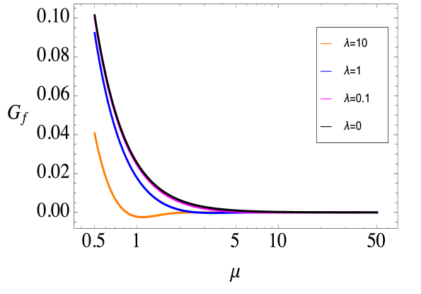
Figure 1: The Green’s function of massless non-local scalar field in flat four space-time dimensions. The propagator is plotted for various strength of non-locality $\lambda$ against the geodesic length $\mu(x,x^{\prime})$.

In the case when $m\neq 0$ things are complicated. Here two possibilities arises $m^{4}>4\lambda^{2}$ and $4\lambda^{2}>m^{4}$, where both $m$ and $\lambda$ are positive. In the former case one can take limit $\lambda\to 0$ (locality limit), while in later case one can take the limit $m\to 0$ (massless limit). In the locality limit, $r_{-}^{2}=0$ and $r_{+}^{2}=m^{2}$. In this case $A=0$ while $B=1$ ($\alpha=\beta=m^{2}/2$). In this case one gets the propagator for local massive scalar field which is

$$G_{f}^{\lambda=0}=(2\pi)^{-d/2}\left(\frac{m}{\mu}\right)^{(d-2)/2}K_{\frac{d}{2}-1}(m\mu)\,,$$ (12)

where $K_{d/2-1}$ is the modified Bessel function of the second kind. It is still possible to perform the above integration for $m\neq 0$ in closed form. For the massive non-local scalar field in arbitrary space-time dimension this Green’s function $G_{f}$ is given by,

$$G_{f}^{m}(x,x^{\prime})=\frac{(2\pi)^{-d/2}\mu^{1-d/2}}{(r_{+}^{2}-r_{-}^{2})}\biggl{[}r_{+}^{d/2+1}K_{\frac{d}{2}-1}\left(r_{+}\mu\right)-r_{-}^{d/2+1}K_{\frac{d}{2}-1}\left(r_{-}\mu\right)\biggr{]}\,,$$ (13)

where $r_{+}$ and $r_{-}$ are stated before and $K_{d/2-1}$ is the modified Bessel function of the second kind. In the limit $\lambda\to 0$ this gives smoothly the result stated in eq. (12). The $m\to 0$ limit of this is smooth and obtains the massless non-local propagator for the scalar theory in arbitrary dimension which agrees with the expression mentioned in eq. (11). The expression in arbitrary dimensions is given by,

$$G_{f}(x,x^{\prime})=\frac{i\left[-\left(i\lambda\right)^{\frac{d+2}{4}}K_{1-\frac{d}{2}}\left(\sqrt{i\lambda}\mu\right)+(-i\lambda)^{\frac{d+2}{4}}K_{\frac{d}{2}-1}\left(\sqrt{-i\lambda}\mu\right)\right]}{2(2\pi)^{d/2}\lambda\mu^{d/2-1}}\,.$$ (14)

In Fig. 2 we plot the massive Green’s function for cases: $m^{2}>2\lambda$, $m^{2}=2\lambda$, $m^{2}<2\lambda$ and $\lambda=0$ (local). The equality case $m^{2}=2\lambda$ is obtained as a limit as has been explained before.

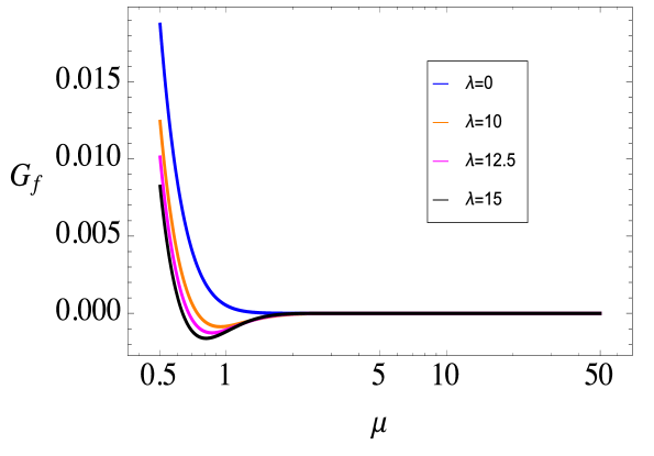
Figure 2: The Green’s function of massive scalar field for non-local theory in flat space-time. The propagator is plotted for various strength of non-locality $\lambda$ against the geodesic length $\mu(x,x^{\prime})$. The four cases plotted are: $m^{2}>2\lambda$, $m^{2}=2\lambda$, $m^{2}<2\lambda$ and $\lambda=0$ (local).

II.2 DeSitter

In this section we will investigate the theory eq. (2 on dS background. The $d$-dimensional deSitter space-time can be identified with the real one-sheeted hyperboloid in $(d+1)$ Minkowski space-time $M_{d+1}$: $X_{d}=\{x\in\mathbb{R}^{d+1},x^{2}=-H^{2}\}$, where $H$ is the Hubble constant. If the two points are denoted by $x$ and $x^{\prime}$, the length of geodesic connecting them is $\mu(x,x^{\prime})$. It is useful to introduce a quantity $z(x,x^{\prime})=\cos^{2}(H\mu/2)$. For space-like distances $\mu^{2}>0$ results in $0<z<1$, while for time-like separation $\mu^{2}<0$ correspond to $1<z<\infty$. Also by making use of the co-ordinates of the embedding space it is noted that the

$$\cos(H\mu)=Z(x,x^{\prime})\,,\hskip 14.22636ptZ(x,x^{\prime})=\eta_{AB}X^{A}(x)X^{B}(x^{\prime})\,$$ (15)

is the embedding distance, i.e. length of chord between the point $x$ and $x^{\prime}$ in the embedding space $\mathbb{R}^{d+1}$. The parameter $z(x,x^{\prime})=(1+Z)/2$. The nice property of maximally symmetric spaces is that Green’s function on such space-time become entirely a function of $\mu$ (or $z(x,x^{\prime})$) instead of being a function of both $x$ and $x^{\prime}$. This allows one to compute Green’s function exactly by solving linear differential equations.

In the case of non-local theory, the Green’s function equation is given in eq. (3). But before we solve for $G(x,x^{\prime})$ on dS, we first note the following important identities on curved space-time.

$$-[\Box^{2}-m^{2}\Box+\lambda^{2}]^{-1}\Box=A(-\Box+r_{-}^{2})^{-1}+B(-\Box+r_{+}^{2})^{-1}\,,$$ (16)

where $A$, $B$, $r_{-}^{2}$ and $r_{+}^{2}$ have the same values as in flat space-time. This is easy to prove by noticing that $-\Box$ can be written in following way

$$-\Box=A(-\Box+r_{+}^{2})+B(-\Box+r_{-}^{2})\,.$$ (17)

This follows from the values of $A$ and $B$ stated in eq. (7) which gives $Ar_{+}^{2}+Br_{-}^{2}=0$ and $A+B=1$. Using $[\Box^{2}-m^{2}\Box+\lambda^{2}]=(-\Box+r_{-}^{2})(-\Box+r_{+}^{2})$ one then immediately obtains the identity stated in eq. (16). This proof is valid as long as $m^{2}\neq 2\lambda$, in the case of equality $m^{2}=2\lambda$ one has follow similar steps described previously for flat space-time. In the case of equality $m^{2}=2\lambda$, the LHS of eq. (16) can be expressed as,

$$-(\Box-\lambda)^{-2}\Box=-(\Box-\lambda)^{-2}(\Box-\lambda+\lambda)=-(\Box-\lambda)^{-1}-\lambda(\Box-\lambda)^{-2}\,.$$ (18)

The RHS of eq. (18) can also be obtained from RHS of eq. (16) by writing $m^{2}=2\lambda+\rho$ and doing a small $\rho$ expansion. Then again the expansion of $A$ and $B$ will be given by eq. (II.1) while we have

$$(-\Box+r_{\pm}^{2})^{-1}=(-\Box+\lambda)^{-1}\mp\sqrt{\lambda\rho}(-\Box+\lambda)^{-2}+\cdots\,.$$ (19)

On plugging these expansions back in eq. (16) it is noticed that divergent piece cancels (as in flat space-time) leaving behind a finite $\rho\to 0$ limit, which matches the RHS of eq. (18). This observation will be useful later in computing the Green’s function on the dS for the case of $m^{2}=2\lambda$.

The identity in eq. (16) is valid for $\lambda\neq 0$. In the case when $\lambda=0$ the operator on LHS reduces to just $\Box+m^{2}$ which is the operator for the local massive scalar field. It is the identify in eq. (16) which allows us to compute the Green’s function of the non-local theory in deSitter space-time. This means that the full Green’s function for non-local theory $G_{NL}(x,x^{\prime})$ is a sum of two Green’s function

$$G_{NL}(x,x^{\prime})=AG_{1}(x,x^{\prime})+BG_{2}(x,x^{\prime})\,,$$ (20)

where

$$(-\Box+r_{-}^{2})G_{1}(x,x^{\prime})=0\,,\hskip 14.22636pt(-\Box+r_{+}^{2})G_{2}(x,x^{\prime})=0\,.$$ (21)

These two Green’s function can be easily computed using the standard methods of computing Green’s function for massive scalar field on deSitter space-time. For example, in the case of local massive scalar field we have $(-\Box+m^{2})G(x,x^{\prime})=0$ as Green’s function equation. In this case by exploiting the knowledge that $G(x,x^{\prime})=G(z(x,x^{\prime}))$, the operator when acting on $G$ acquires the following hyper-geometric form

$$z(1-z)G^{\prime\prime}+\left[c-(a+b+1)z\right]G^{\prime}-abG=0\,,$$ (22)

where $G^{\prime}={\rm d}G(z)/{\rm d}z$, $a=\bigl{[}d-1+\bigl{(}(d-1)^{2}-4m^{2}/H^{2}\bigr{)}^{1/2}\bigr{]}/2$, $b=\bigl{[}d-1-\bigl{(}(d-1)^{2}-4m^{2}/H^{2}\bigr{)}^{1/2}\bigr{]}/2$ and $c=d/2$. This is a Hyper-geometric differential equation of second order and has two linearly independent solution: ${}_{2}F_{1}(a,b,c;z)$ and ${}_{2}F_{1}(a,b,c;1-z)$ Allen:1985ux ; Allen:1985wd ; Allen:1987tz . The former has a singularity at $z=1$ (which corresponds to short distance $\mu=0$) while the later is singular at $z=0$ (corresponding to antipodal separation). By requiring the short distance singularity of dS propagator to match with the singular behaviour of the flat space-time propagator, and being regular at $z=0$, one concludes that $G(z)=q\times{}_{2}F_{1}(a,b,c;z)$ (where $q$ is to be fixed by requiring that the strength of singularity of dS propagator to match with the strength of singularity in flat space-time). The coefficient $q$ is given by,

$$q=\frac{H^{d-2}\Gamma(a)\Gamma(b)}{(4\pi)^{d/2}\Gamma(c)}\,.$$ (23)

Using this one can write the Green’s function $G_{NL}$ for non-local scalar on dS to be

$$G_{NL}(z)=Aq\,{}_{2}F_{1}(a_{1},b_{1},c_{1};z)+B\bar{q}\,{}_{2}F_{1}(a_{2},b_{2},c_{2};z)\,,$$ (24)

where the coefficients $q$ and $\bar{q}$ are obtained from eq. (23) by making transformation $m^{2}\to r_{-}^{2}$ and $m^{2}\to r_{+}^{2}$ respectively, while

$$a_{1}=\frac{1}{2}\bigl{[}d-1+\sqrt{(d-1)^{2}-\frac{4r_{-}^{2}}{H^{2}}}\bigr{]}\,, b_{1}=\frac{1}{2}\bigl{[}d-1-\sqrt{(d-1)^{2}-\frac{4r_{-}^{2}}{H^{2}}}\bigr{]}\,, c_{1}=d/2\,,$$

$$a_{2}=\frac{1}{2}\bigl{[}d-1+\sqrt{(d-1)^{2}-\frac{4r_{+}^{2}}{H^{2}}}\bigr{]}\,, b_{2}=\frac{1}{2}\bigl{[}d-1-\sqrt{(d-1)^{2}-\frac{4r_{+}^{2}}{H^{2}}}\bigr{]}\,, c_{2}=d/2\,.$$ (25)

The values of $q$ and $\bar{q}$ so obtained can be plugged back in eq. (24) to obtain the full non-local Green’s function on dS for space-like separation ($0<z<1$). This is the propagator for arbitrary mass $m$, $\lambda$ and $d$.

The beautiful thing about the presence of non-locality (however small) is that it allows us to take a smooth massless limit on deSitter, which is not possible in case of local scalar field theory on deSitter. This is the main and most important result of this paper. Moreover, the Green’s function for non-local massless scalar field computed directly (by starting from a non-local massless theory directly), agrees exactly with the case of massive non-local Green’s function in limit $m\to 0$. This beautiful smooth limit is due to the lack of zero modes in the case of non-local scalar field theory, which is not so in local case. This massless limit is given by,

$$\left.G_{NL}\right|_{m\to 0}=\frac{H^{d-2}}{2(4\pi)^{d/2}}\left[\Gamma(a_{1})\Gamma(b_{1}){}_{2}\tilde{F}_{1}(a_{1},b_{1},c_{1};z)+\Gamma(a_{2})\Gamma(b_{2}){}_{2}\tilde{F}_{1}(a_{2},b_{2},c_{2};z)\right]\,,$$ (26)

where the parameters $a_{1}$, $b_{1}$, $c_{1}$, $a_{2}$, $b_{2}$ and $c_{2}$ here are determined from eq. (II.2) in the limit $m\to 0$. In Figure 3 we plot this Green’s function for various values of $\lambda_{s}$.

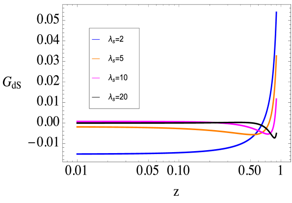
Figure 3: The Green’s function of massless scalar field for non-local theory in deSitter space-time. The propagator is plotted for various strength of non-locality $\lambda_{s}=\lambda/H^{2}$ against $z(x,x^{\prime})$.

For the case of non-zero mass, the propagator has one more parameter, however structure remains same. Here we have three cases (as in flat space-time): $m^{2}<2\lambda$, $m^{2}=2\lambda$ and $m^{2}>2\lambda$. In each case the propagator is real for space-like separation. It is worthwhile to plot the propagator for fixed value of $\lambda_{s}$ and for decreasing mass. It is seen that as $m\to 0$, the massive propagator smoothly approaches the massless non-local propagator. In figure. 4 we plot this scenario.

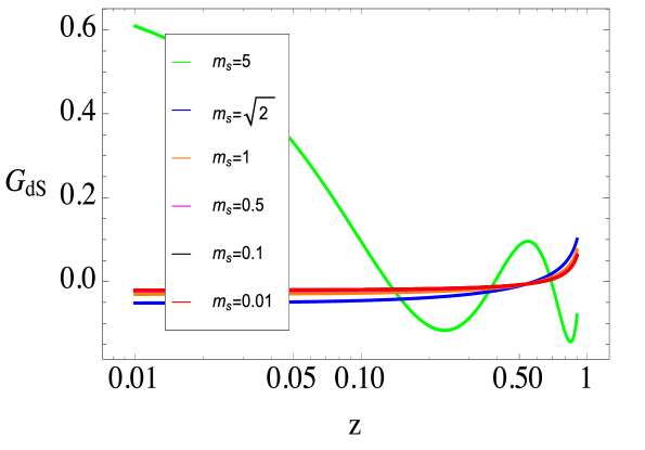
Figure 4: The Green’s function of non-local scalar field theory in deSitter space-time. Here we slowly take the $m\to 0$ limit. We plot the three cases: $m^{2}>2\lambda$, $m^{2}=2\lambda$ and $m^{2}<2\lambda$. In the last case we plot the propagator for decreasing values of $m$ to indicate the smooth massless limit. The propagator is plotted for fixed $\lambda$ and various values of decreasing $m$.

The case of equality is interesting as then the propagator depends only on one parameter. Physically it implies that the two length scales are comparable. In this case the non-locality scale is coupled with the mass, so $m\to 0$ implies $\lambda\to 0$ simultaneously. In this equality case, as has been discussed before, we have $r_{-}^{2}=r_{+}^{2}=m^{2}/2$. This implies that $a_{1}=a_{2}$, $b_{1}=b_{2}$, while $A$ and $B$ diverges. This divergence in $A$ and $B$ has been discussed before, and it is not a problematic thing as it cancels off. As before we can define $m^{2}=2\lambda+\rho$ and compute the propagator. Expanding the propagator in powers of $\rho$ clearly shows the absence of any divergence which is expected as shown previously, the way eq. (16) reduces to eq. (18) in the limit $\rho\to 0$. The Green’s function can then be obtained by taking the limit $\rho\to 0$. The Green’s function obtained in this limit is well-defined and analytic. In figure 4 the case of $m_{s}=m/H=\sqrt{2}$ refers to this scenario.

To obtain the propagator for time-like separation (or Feynman propagator) we consider two cases: $G_{NL}(z+i\epsilon)$ and $G_{NL}(z-i\epsilon)$ (as for $z>1$ the hypergeometric function has branch-cut on the real axis) Allen:1985ux ; Allen:1985wd ; Allen:1987tz . The Feynman propagator $G_{NL}^{F}(z)=\lim_{\epsilon\to 0}G_{NL}(z+i\epsilon)$, while the symmetric propagator is $G_{NL}^{S}(z)=\lim_{\epsilon\to 0}\{G_{NL}(z+i\epsilon)+G_{NL}(z-i\epsilon)\}$.

II.3 Large time behaviour

It is important to check how the propagator in non-local theory behaves at large time. To investigate this one has to write the propagator in Lorentzian signature. For this one can first write the dS metric in either flat or static co-ordinates system. We consider static co-ordinate system:

$${\rm d}s^{2}=-(1-H^{2}r^{2}){\rm d}t^{2}+\frac{{\rm d}r^{2}}{(1-H^{2}r^{2})}+r^{2}{\rm d}\Omega^{2}\,.$$ (27)

The embedding map between the 5D bulk space $X^{\alpha}$ ($\alpha=0,\cdots,4$) and the static patch $x^{\mu}=(t,r,\theta,\phi)$ is:

$$X^{0}=\sqrt{1-H^{2}r^{2}}\sinh(Ht)\,, X^{1}=r\sin\theta\cos\phi\,, X^{2}=r\sin\theta\sin\phi\,,$$

$$X^{3}=r\cos\theta\,, X^{4}=\sqrt{1-H^{2}r^{2}}\cosh(Ht)\,,$$ (28)

where $1\leq Hr\leq 1$, $0\leq\theta\leq\pi$ and $0\leq\phi\leq 2\pi$. These transformation then imply that the parameter $z(x,x^{\prime})$ can be computed using eq. (15) which is given by

$$2z-1=\sqrt{(1-H^{2}r^{2})(1-H^{2}r^{\prime 2})}\cosh(H(t-t^{\prime}))+H^{2}rr^{\prime}\cos\Omega\,,$$ (29)

where

$$\cos\Omega\equiv\cos\theta\cos\theta^{\prime}+\sin\theta\sin\theta^{\prime}\cos(\phi-\phi^{\prime})\,.$$ (30)

Then to study the large time behaviour of the Green’s function $G(x,x^{\prime})$ we just fix one co-ordinate and take the other to large distance. To achieve this we choose the following configuration

$$x:\{t=T,r=r,\theta=0,\phi=0\}\,,\hskip 14.22636ptx^{\prime}:\{t^{\prime}=0,r^{\prime}=r,\theta^{\prime}=0,\phi^{\prime}=0\}\,.$$ (31)

This gives for time-like separation (where one has to take in to account the proper $i\epsilon$-prescription)

$$z(x,x^{\prime})=\frac{1+Z}{2}=\cosh^{2}\left(\frac{HT}{2}\right)-H^{2}r^{2}\sinh^{2}\left(\frac{HT}{2}\right)+i\epsilon\approx\frac{e^{HT}}{4}(1-H^{2}r^{2})+i\epsilon\,.$$ (32)

Using this one can now study the large $T$ behaviour of the Green’s function by plugging $z(x,x^{\prime})$ in to the expression for Green’s function $G_{NL}(z)$. Furthermore, if $r=0$ then $z$ only gets contribution from $T$. In this sense for time-like separation, the large $T$ corresponds to large $z(x,x^{\prime})$. Our Green’s function is a linear combination of two hyper-geometric functions as indicated in eq. (24) where $q$ and $\bar{q}$ are constants depending on parameters of the theory. The large-$z$ expansion of hypergeometric functions are well known in literature. For example for ${}_{2}F_{1}(a,b,c;z)$ in $z\to\infty$ gives

$${}_{2}F_{1}(a,b,c;z)= \frac{\Gamma(c)\Gamma(b-a)}{\Gamma(b)\Gamma(c-a)}(-z)^{-a}{}_{2}F_{1}(a,a-c+1,a-b+1;z^{-1})$$

$$+\frac{\Gamma(c)\Gamma(a-b)}{\Gamma(a)\Gamma(c-b)}(-z)^{-b}{}_{2}F_{1}(b,b-c+1,b-a+1;z^{-1})\,,$$ (33)

where $\lvert\arg(1-z)\rvert<\pi$. This is true when $(a-b)$ is not an integer. For massless local scalar theory this condition is not satisfied as $(a-b)$ is an integer in any space-time dimensions. Then the asymptotic expansion of hyper-geometric functions gets an additional factor of $\log z$. This $\log z$ factor is the source of IR divergence when $z\to\infty$. In case when non-locality is present $(a-b)$ is never integer for any space-time dimensions. As a result $\log z$ factor doesn’t arise in asymptotic expansion of hyper-geometric functions thereby implying absence of dangerous IR $\log$-divergence.

This identity can be utilised to express the large-$T$ behaviour of the non-local Green’s function. This will imply that for $z\to\infty$

$$G_{NL}(z)= \frac{q\Gamma(c_{1})\Gamma(b_{1}-a_{1})}{\Gamma(b_{1})\Gamma(c_{1}-a_{1})}(-z)^{-a_{1}}{}_{2}F_{1}(a_{1},a_{1}-c_{1}+1,a_{1}-b_{1}+1;z^{-1})$$

$$+\frac{q\Gamma(c_{1})\Gamma(a_{1}-b_{1})}{\Gamma(a_{1})\Gamma(c_{1}-b_{1})}(-z)^{-b_{1}}{}_{2}F_{1}(b_{1},b_{1}-c_{1}+1,b_{1}-a_{1}+1;z^{-1})$$

$$+\frac{\bar{q}\Gamma(c_{2})\Gamma(b_{2}-a_{2})}{\Gamma(b_{2})\Gamma(c_{2}-a_{2})}(-z)^{-a_{2}}{}_{2}F_{1}(a_{2},a_{2}-c_{2}+1,a_{2}-b_{2}+1;z^{-1})$$

$$+\frac{\bar{q}\Gamma(c_{2})\Gamma(a_{2}-b_{2})}{\Gamma(a_{2})\Gamma(c_{2}-b_{2})}(-z)^{-b_{2}}{}_{2}F_{1}(b_{2},b_{2}-c_{2}+1,b_{2}-a_{2}+1;z^{-1})\,.$$ (34)

Plugging eq. (32) in eq. (II.3) we get the behaviour of the non-local Green’s function at large time-like separations. This is given by,

$$G_{NL}\rvert_{z\to\infty}=\frac{q\Gamma(c_{1})\Gamma(b_{1}-a_{1})(-\gamma)^{-a_{1}}}{\Gamma(b_{1})\Gamma(c_{1}-a_{1})}e^{-a_{1}HT}+\frac{q\Gamma(c_{1})\Gamma(a_{1}-b_{1})(-\gamma)^{-b_{1}}}{\Gamma(a_{1})\Gamma(c_{1}-b_{1})}e^{-b_{1}HT}$$

$$+\frac{\bar{q}\Gamma(c_{2})\Gamma(b_{2}-a_{2})(-\gamma)^{-a_{2}}}{\Gamma(b_{2})\Gamma(c_{2}-a_{2})}e^{-a_{2}HT}+\frac{\bar{q}\Gamma(c_{2})\Gamma(a_{2}-b_{2})(-\gamma)^{-b_{2}}}{\Gamma(a_{2})\Gamma(c_{2}-b_{2})}e^{-b_{2}HT}\,,$$ (35)

where $\gamma=(1-H^{2}r^{2})/4$. As $T\to\infty$ each of these terms get exponentially suppressed resulting in IR well-behaved Green’s function even for massless theory. This is possible due to the presence of non-locality. This implies that the Green’s function on dS in the presence of non-locality respect cluster-decomposition theorem as correlation exponentially decays at large time-like separations.

III Conclusions

In this letter we considered non-local scalar field theory on flat and de Sitter space-time. We computed the propagator of scalar field in either case, for both massless and massive theories. It is seen that the limit $m\to 0$ is smooth in presence of non-locality on dS. Moreover, the $m\to 0$ limit of propagator of massive non-local scalar field matches exactly with the massless non-local propagator for both flat and dS space-time. This offers an interesting solution to the long-standing problem of infrared divergence for scalar field theories on dS. It is seen that no divergence arises in the limit $m\to 0$ in the presence of non-locality however small. Furthermore, it is seen that the correlation of two fields decays exponentially at large time-like separations, and the presence of non-locality doesn’t give rise to dangerous $\log z$ divergent in massless theories which is the case in local theories. In this way the presence of non-locality leads to infrared divergence free Green’s function. It shows that the Green’s function of the non-local theory obeys cluster decomposition theorem. These are the two most important results of the paper. It shows that non-locality may hold the key to cure the IR issues of field theory in dS space-time.

This opens up several future directions. There has been no systematic study of low energy non-local modifications of field theories in de Sitter space-time. Our result suggests that this subject merits further investigation. It is interesting to ask whether this result holds for a larger class of non-local field theories. Furthermore, it will be worth investigating interacting theories in the presence of non-locality and study low energy effective action of such theories which is expected to get modified due to IR non-locality at large distances.

Acknowledgements

GN will like to thank Alok Laddha for useful discussions. NK is supported by the SERB National Postdoctoral Fellowship. GN is supported by “Zhuoyue” (Distinguished) Fellowship (ZYBH2018-03).

References

- (1) A. H. Guth, Phys. Rev. D 23, 347 (1981) [Adv. Ser. Astrophys. Cosmol. 3, 139 (1987)]. doi:10.1103/PhysRevD.23.347
- (2) A. D. Linde, Phys. Lett. 108B, 389 (1982) [Adv. Ser. Astrophys. Cosmol. 3, 149 (1987)]. doi:10.1016/0370-2693(82)91219-9
- (3) A. A. Starobinsky, Phys. Lett. 117B, 175 (1982). doi:10.1016/0370-2693(82)90541-X
- (4) A. G. Riess et al. [Supernova Search Team], Astron. J. 116, 1009 (1998) doi:10.1086/300499 [astro-ph/9805201].
- (5) S. Perlmutter et al. [Supernova Cosmology Project Collaboration], Astrophys. J. 517, 565 (1999) doi:10.1086/307221 [astro-ph/9812133].
- (6) Y. Akrami et al. [Planck Collaboration], arXiv:1807.06205 [astro-ph.CO].
- (7) N. Aghanim et al. [Planck Collaboration], arXiv:1807.06209 [astro-ph.CO].
- (8) N. A. Chernikov and E. A. Tagirov, Ann. Inst. H. Poincare Phys. Theor. A 9, 109 (1968).
- (9) T. S. Bunch and P. C. W. Davies, Proc. Roy. Soc. Lond. A 360, 117 (1978). doi:10.1098/rspa.1978.0060
- (10) B. Allen, Phys. Rev. D 32, 3136 (1985). doi:10.1103/PhysRevD.32.3136
- (11) J. Bros, U. Moschella and J. P. Gazeau, Phys. Rev. Lett. 73, 1746 (1994). doi:10.1103/PhysRevLett.73.1746
- (12) J. Serreau, Phys. Rev. Lett. 107, 191103 (2011) doi:10.1103/PhysRevLett.107.191103 [arXiv:1105.4539 [hep-th]].
- (13) J. Bros, H. Epstein and U. Moschella, Lett. Math. Phys. 93, 203 (2010) doi:10.1007/s11005-010-0406-4 [arXiv:1003.1396 [hep-th]].
- (14) D. Marolf and I. A. Morrison, Phys. Rev. D 82, 105032 (2010) doi:10.1103/PhysRevD.82.105032 [arXiv:1006.0035 [gr-qc]].
- (15) E. T. Akhmedov, Int. J. Mod. Phys. D 23, 1430001 (2014) doi:10.1142/S0218271814300018 [arXiv:1309.2557 [hep-th]].
- (16) B. Allen and T. Jacobson, Commun. Math. Phys. 103, 669 (1986). doi:10.1007/BF01211169
- (17) B. Allen and A. Folacci, Phys. Rev. D 35, 3771 (1987). doi:10.1103/PhysRevD.35.3771
- (18) I. Antoniadis, J. Iliopoulos and T. N. Tomaras, Phys. Rev. Lett. 56, 1319 (1986). doi:10.1103/PhysRevLett.56.1319
- (19) A. Folacci, Phys. Rev. D 46, 2553 (1992) doi:10.1103/PhysRevD.46.2553 [arXiv:0911.2064 [gr-qc]].
- (20) K. Kirsten and J. Garriga, Phys. Rev. D 48, 567 (1993) doi:10.1103/PhysRevD.48.567 [gr-qc/9305013].
- (21) M. B. Einhorn and D. R. T. Jones, JHEP 1703, 144 (2017) doi:10.1007/JHEP03(2017)144 [arXiv:1606.02268 [hep-th]].
- (22) M. B. Einhorn and F. Larsen, Phys. Rev. D 67, 024001 (2003) doi:10.1103/PhysRevD.67.024001 [hep-th/0209159].
- (23) A. Rajaraman, J. Kumar and L. Leblond, Phys. Rev. D 82, 023525 (2010) doi:10.1103/PhysRevD.82.023525 [arXiv:1002.4214 [hep-th]].
- (24) S. Hollands, Annales Henri Poincare 13, 1039 (2012) doi:10.1007/s00023-011-0140-1 [arXiv:1105.1996 [gr-qc]].
- (25) F. Gautier and J. Serreau, Phys. Lett. B 727, 541 (2013) doi:10.1016/j.physletb.2013.10.072 [arXiv:1305.5705 [hep-th]].
- (26) A. Youssef and D. Kreimer, Phys. Rev. D 89, 124021 (2014) doi:10.1103/PhysRevD.89.124021 [arXiv:1301.3205 [gr-qc]].
- (27) L. Modesto, Phys. Rev. D 86, 044005 (2012) doi:10.1103/PhysRevD.86.044005 [arXiv:1107.2403 [hep-th]].
- (28) L. Modesto and L. Rachwa?, Int. J. Mod. Phys. D 26, no. 11, 1730020 (2017). doi:10.1142/S0218271817300208
- (29) S. Deser and R. P. Woodard, Phys. Rev. Lett. 99, 111301 (2007) doi:10.1103/PhysRevLett.99.111301 [arXiv:0706.2151 [astro-ph]].
- (30) S. Capozziello, E. Elizalde, S. Nojiri and S. D. Odintsov, Phys. Lett. B 671, 193 (2009) doi:10.1016/j.physletb.2008.11.060 [arXiv:0809.1535 [hep-th]].
- (31) S. Deser and R. P. Woodard, JCAP 1311, 036 (2013) doi:10.1088/1475-7516/2013/11/036 [arXiv:1307.6639 [astro-ph.CO]].
- (32) R. P. Woodard, Found. Phys. 44, 213 (2014) doi:10.1007/s10701-014-9780-6 [arXiv:1401.0254 [astro-ph.CO]].
- (33) E. Elizalde, E. O. Pozdeeva and S. Y. Vernov, Phys. Rev. D 85, 044002 (2012) doi:10.1103/PhysRevD.85.044002 [arXiv:1110.5806 [astro-ph.CO]].
- (34) M. Maggiore, Fundam. Theor. Phys. 187, 221 (2017) doi:10.1007/978-3-319-51700-116 [arXiv:1606.08784 [hep-th]].
- (35) G. Narain and T. Li, Phys. Rev. D 97, no. 8, 083523 (2018) doi:10.1103/PhysRevD.97.083523 [arXiv:1712.09054 [hep-th]].
- (36) G. Narain and T. Li, Universe 4, no. 8, 82 (2018) doi:10.3390/universe4080082 [arXiv:1807.10028 [hep-th]].
- (37) N. Kajuri, Phys. Rev. D 95, no. 10, 101701 (2017) doi:10.1103/PhysRevD.95.101701 [arXiv:1704.03793 [gr-qc]].
- (38) N. Kajuri and D. Kothawala, arXiv:1806.10345 [gr-qc].
- (39) J. Maldacena and G. L. Pimentel, JHEP 1302, 038 (2013) doi:10.1007/JHEP02(2013)038 [arXiv:1210.7244 [hep-th]].
- (40) A. Matsumura and Y. Nambu, Phys. Rev. D 98, no. 2, 025004 (2018) doi:10.1103/PhysRevD.98.025004 [arXiv:1707.08414 [gr-qc]].