Rescuing Quartic and Natural Inflation
in the Palatini Formalism

Abstract

When considered in the Palatini formalism, the Starobinsky model does not provide us with a mechanism for inflation due to the absence of a propagating scalar degree of freedom. By (non)–minimally coupling scalar fields to the Starobinsky model in the Palatini formalism we can in principle describe the inflationary epoch. In this article, we focus on the minimally coupled quartic and natural inflation models. Both theories are excluded in their simplest realization since they predict values for the inflationary observables that are outside the limits set by the Planck data. However, with the addition of the $R^{2}$ term and the use of the Palatini formalism, we show that these models can be rendered viable.

1 Introduction

Cosmological inflation [1, 2, 3, 4, 5, 6, 7], namely a phase of de Sitter expansion after the big bang, provides an attractive paradigm addressing the open issues of the early universe. In this framework quantum fluctuations, magnified to a cosmic size, ultimately generate the large scale structure of the universe and the presently observed anisotropy in the CMB. Although a detailed particle physics mechanism underlying inflation has not been established yet, models of inflation formulated in terms of a scalar degree of freedom (inflaton) exist with a number of predictions confirmed by observations. This scalar degree of freedom is introduced either as a fundamental scalar field or can be provided by gravity itself in models featuring generalizations of the Einstein-Hilbert action. The latter possibility is realized in the Starobinsky model where an extra quadratic term of the Ricci curvature scalar $R^{2}$ is present. Among the models realizing the former possibility of a fundamental scalar, the case of Higgs inflation [8, 9, 10, 11, 12, 13, 14, 15, 16, 17, 18, 19, 20, 21, 22, 23, 24, 25], where the inflaton is identified with the Standard Model Higgs boson, has attracted a lot of attention since it provides a direct connection of cosmological inflation to particle physics. Higgs inflation requires the presence of an appreciable coupling of the Higgs field $h$ to the Ricci curvature scalar $\xi h^{2}R$.

Both of the above possibilities are intimately connected with gravitation and its formulation. It is well known that for the Einstein-Hilbert action of pure gravitation the alternative variational principle of Palatini [26, 27, 28, 29, 30], in which not only the metric $g_{\mu\nu}$ but also the connection $\Gamma_{\mu\nu}^{\rho}$ are treated as independent variables, leads to the standard equations of motion of General Relativity (GR) and the Palatini formulation is equivalent to the standard metric formulation. Nevertheless, this is not the case when extra fields are coupled to gravity non-minimally as in the case of Higgs inflation. New interactions in the scalar sector modifying significantly the Einstein-frame potential are present in the Palatini formulation. The inequivalence of the two formulations is also quite striking in the case of the Starobinsky model, where, in the Palatini formulation there is no propagating extra scalar degree of freedom, in contrast to the metric formulation, where the quadratic curvature term introduces an extra scalar suitable to play the role of the inflaton.

In the present article we consider scalar matter coupled to gravity in the framework of the Palatini formulation (see [31] for a review and [30, 32, 33, 34, 35, 36, 37, 38, 39, 40, 41, 42, 43, 44, 45, 25, 46, 47, 48, 49, 50, 51, 52, 53, 54, 55] for various applications). We focus on the case that a quadratic Starobinsky term is present while the scalar fields are minimally coupled to gravity. We analyze the case of a model with quartic scalar interactions, a case of interest to Higgs inflation. We find acceptable slow-roll inflationary behaviour, despite the fact that scalars are minimally coupled to gravity, contrary to the standard metric case where an appreciable non-minimal coupling is required. The central ingredient of the inflation mechanism operating in the Palatini framework for a model described by a potential $V(\phi)$ is the creation of a plateau for the Einstein-frame potential $\bar{V}(\phi)=V(\phi)/\left(1+4\alpha V(\phi)/M_{P}^{4}\right)$ at large field values [52, 46]. We extend our analysis to the case of the natural inflation model [74, 75] characterized by a bounded potential and find that the resulting flattening of the inflationary plateau in the Palatini formulation leads to acceptable slow-roll inflationary behaviour.

The paper is organized as follows: In section 2 we start with the action of a scalar field minimally coupled to gravity in the presence of a quadratic curvature scalar term with a general self-interacting potential and derive the Einstein frame Lagrangian in the framework of the Palatini formalism. In section 3.1 we consider the case of a quartic potential modelled in the fashion of the Higgs boson and proceed to analyze the inflationary behaviour calculating the slow-roll parameters and the corresponding inflationary observables. Also, in section 3.2 we briefly discuss other monomial potentials. Then, in section 4 we analyze the natural inflation model. Finally, in section 5 we present our conclusions.

2 Minimally Coupled Scalars in the Palatini Formalism

Consider the action of scalar fields minimally coupled to gravity. Although we restrict our consideration to one scalar, the generalization to many is straightforward. We have

$${\cal{S}}_{0}\,=\,\int\,d^{4}x\,\sqrt{-g}\,\left\{\,\frac{1}{2}M_{P}^{2}\,R\,-\frac{1}{2}\left(\nabla\phi\right)^{2}\,-V(\phi)\,\right\}\ .{}$$ (2.1)

We expect that quantum corrections are bound to generate in (2.1) terms of the form $\xi\phi^{2}R$ and $\alpha R^{2}$. Either of these terms has been shown to lead to a number of interesting results with respect to inflation. It is conceivable though, since the phenomenological values of the parameters $\xi$ and $\alpha$ are not a priori known, that one or both of these terms are small or negligible. In what follows we shall focus on the case of a negligible non-minimal coupling, i.e. take $\xi=0$, and consider the action

$${\cal{S}}\,=\,\int\,d^{4}x\,\sqrt{-g}\,\left\{\,\frac{1}{2}M_{P}^{2}\,R\,+\,\frac{\alpha}{4}R^{2}\,-\frac{1}{2}\left(\nabla\phi\right)^{2}\,-V(\phi)\,\right\}\ ,{}$$ (2.2)

which can be readily written in terms of an auxiliary scalar field $\chi$ as

$${\cal{S}}\,=\,\int\,d^{4}x\,\sqrt{-g}\,\left\{\,\frac{1}{2}M_{P}^{2}\left(1+\alpha\chi^{2}\right)R\,-\frac{\alpha}{4}\chi^{4}\,-\frac{1}{2}\left(\nabla\phi\right)^{2}\,-V(\phi)\,\right\}\ .{}$$ (2.3)

We shall consider the above action in the framework of the Palatini or first order formalism in which, next to the metric $g_{\mu\nu}$, the connection $\Gamma_{\mu\nu}^{\rho}$ also is an independent variable. Therefore, $R_{\mu\nu}$ is independent of the metric. Performing a Weyl rescaling of the metric according to

$$\bar{g}_{\mu\nu}\,=\,\frac{1}{M_{P}^{2}}\left(M_{P}^{2}+\alpha\chi^{2}\right)\,g_{\mu\nu}\ ,$$ (2.4)

we transform the action(2.3) into the Einstein frame

$${\cal{S}}\,=\,\int\,d^{4}x\,\sqrt{-\bar{g}}\,\left\{\,\frac{1}{2}M_{P}^{2}\,\bar{R}\,-\frac{1}{2}\frac{M_{P}^{2}\left(\overline{\nabla}\phi\right)^{2}}{(M_{P}^{2}+\alpha\chi^{2})}\,-\overline{V}(\phi,\chi)\,\right\}\ ,{}$$ (2.5)

where $\bar{R}=\bar{g}^{\mu\nu}R_{\mu\nu}(\Gamma)$ and

$$\overline{V}(\phi,\chi)\,=\,\frac{M_{P}^{4}\,\left(\,V(\phi)\,+\,\frac{\alpha}{4}\chi^{4}\right)}{\left(M_{P}^{2}+\alpha\chi^{2}\right)^{2}}\ .$$ (2.6)

Variation of the Einstein-Hilbert action (2.5) with respect to the connection yields the standard Levi-Civita relation in terms of the metric $\bar{g}$. The Einstein field equations are the same as in the standard metric formulation. Varying with respect to the auxiliary field $\chi$ we obtain

$$\frac{\delta{\cal{S}}}{\delta\chi}\,=\,0\,\Longrightarrow\,\chi^{2}\,=\,\frac{4V(\phi)\,+\,(\nabla\phi)^{2}}{M_{P}^{2}-\alpha\frac{(\nabla\phi)^{2}}{M_{P}^{2}}}\ .{}$$ (2.7)

Note that we have dropped the bars for the sake of simplicity of notation. Substituting (2.7) into the action (2.5) we obtain

$${\cal{S}}\,=\,\int\,\sqrt{-g}\left\{\,\frac{1}{2}M_{P}^{2}\,R\,-\frac{1}{2}\frac{\left(\nabla\phi\right)^{2}}{\left(1\,+\,\frac{4\alpha}{M_{P}^{4}}V(\phi)\,\right)}\,-\frac{V(\phi)}{\left(1\,+\,\frac{4\alpha}{M_{P}^{4}}V(\phi)\,\right)}\,+\,O((\nabla\phi)^{4})\,\right\}\ .{}$$ (2.8)

Since we aim to study the properties of this action in the framework of slow-roll inflation, higher than quadratic powers of $\nabla\phi$ are not expected to play any role.

The above can be generalized to any $f(R)$ theory replacing the action (2.5) with

$${\cal{S}}\,=\,\int\,d^{4}x\,\sqrt{-g}\,\left\{\,\frac{1}{2}f^{\prime}(\chi^{2})\,R\,-\frac{1}{2}\left(\nabla\phi\right)^{2}\,-V(\phi)\,-U(\chi^{2})\,\right\}\ ,$$ (2.9)

where the derivative is with respect to $\chi^{2}$ and

$$U(\chi^{2})\,=\,\frac{1}{2}\left(\,\chi^{2}\,f^{\prime}(\chi^{2})\,-f(\chi^{2})\,\right)\ .{}$$ (2.10)

Then, the Weyl rescaling factor is replaced by $\Omega^{2}=f^{\prime}(\chi^{2})/M_{P}^{2}$ and (2.7) becomes

$$2f(\chi^{2})\,-\chi^{2}f^{\prime}(\chi^{2})\,-f^{\prime}(\chi^{2})\frac{(\nabla\phi)^{2}}{M_{P}^{2}}\,=\,4V(\phi)\ .$$ (2.11)

3 Application to Higgs-like Scalars

3.1 Quartic potentials

Higgs inflation, i.e. the possibility of the Standard Model Higgs playing the role of the inflaton, has attracted a lot of attention. A necessary requirement of such a scenario within the standard metric formulation is a rather large non-minimal coupling of the Higgs to the Ricci scalar $\xi|H|^{2}R$. In the unitary gauge the Higgs doublet can be replaced by a single scalar $\phi$

$$H\,=\,\frac{1}{\sqrt{2}}\left(\begin{array}[]{c}0\\ \phi\end{array}\right)\,\,\Longrightarrow\,\,\,V(\phi)\,=\,\frac{\lambda}{4}\left(\phi^{2}-v^{2}\right)^{2}\ .{}$$ (3.1)

Of course, if this is to represent a realistic version of the Standard Model, issues like the stability of the Higgs self-coupling have to be addressed, possibly by enlarging the Higgs sector.

In this section we shall consider the case of a scalar $\phi$ with a quartic potential (3.1) minimally coupled to gravity ($\xi=0$) in the framework of the Palatini formalism. The corresponding scalar part of the Lagrangian derived in (2.8) is

$${\cal{L}}(\phi)\,=\,-\frac{1}{2}\frac{(\nabla\phi)^{2}}{\left(1+\frac{\lambda\alpha}{M_{P}^{4}}\left(\phi^{2}-v^{2}\right)^{2}\,\right)}\,-\frac{\frac{\lambda}{4}\left(\phi^{2}-v^{2}\right)^{2}}{\left(1+\frac{\lambda\alpha}{M_{P}^{4}}\left(\phi^{2}-v^{2}\right)^{2}\,\right)}\,+\,O((\nabla\phi)^{4})\ .{}$$ (3.2)

Note that the vanishing of the potential at the (Minkowski) vacuum corresponds through (2.7) to a vanishing of the vacuum expectation value of the auxiliary field $\chi$ and consequently to an equality of the Jordan frame and Einstein frame Planck masses.

The scalar field $\phi$ can be replaced by a canonically normalized field $\zeta$ defined by

$$\zeta\,=\,\int\,\frac{d\phi}{\sqrt{1+\frac{\lambda\alpha}{M_{P}^{4}}\left(\phi^{2}-v^{2}\right)^{2}\,}}\ .{}$$ (3.3)

For very large values of the field $\phi\gg v$ this is approximately

$$\zeta=M_{P}\,(\alpha\lambda)^{-1/4}\int\!\frac{\mathrm{d}x}{\sqrt{1+x^{4}}}\,=\,\frac{M_{P}}{(\alpha\lambda)^{1/4}}\left(\,\frac{4}{\sqrt{\pi}}\left(\Gamma(5/4)\right)^{2}\,-\frac{1}{2}{\cal{F}}(y,1/\sqrt{2})\,\right)\,,$$ (3.4)

where $x\equiv(\alpha\lambda)^{1/4}\phi/M_{P}$, $\cos{y}\equiv(x^{2}-1)/(x^{2}+1)$ and $\mathcal{F}$ refers to the elliptic integral of the first kind. We can invert the above expression and obtain $x(\zeta)$ in terms of one of the Jacobi’s elliptic functions ($sn$). In Fig. 1 we present a plot of $x$ in terms of the normalized canonical field $\bar{\zeta}\equiv(\alpha\lambda)^{1/4}\zeta/M_{P}$.

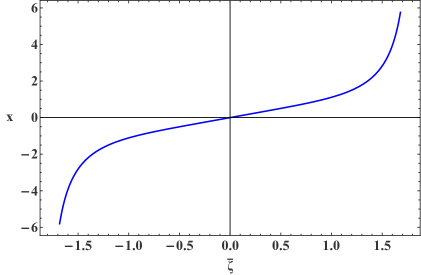
Figure 1: Plot of $x(\bar{\zeta})$.

The $\bar{\zeta}$ function saturates at some value, say $\pm\bar{\zeta}_{0}$, for $x\rightarrow\pm\infty$. This can also be verified analytically, by means of an asymptotic expansion of $\mathcal{F}$ at large $x$ values.

The potential $\bar{V}$ in (3.2) for the large $\phi\gg v$ region, expressed in terms of $x$, reads

$$\bar{V}=\frac{M_{P}^{4}}{4\alpha}\,\frac{x^{4}(\zeta)}{\left(1+x^{4}(\zeta)\right)}\,{}$$ (3.5)

and it is presented in Fig. 2.

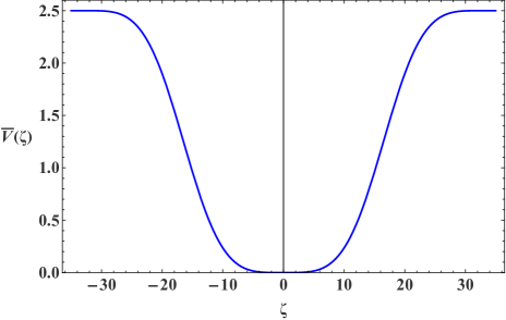
Figure 2: A plot of the potential $\bar{V}(\zeta)$ for $\alpha=0.1$ and $\lambda=10^{-4}$ in natural units.

Next, we proceed to study slow-roll inflation for this particular model. Substituting the above potential in the slow-roll parameters

$$\epsilon_{V}=\frac{M_{P}^{2}}{2}\left(\frac{\bar{V}^{\prime}(\zeta)}{\bar{V}(\zeta)}\right)^{2},\qquad\eta_{V}=M_{P}^{2}\left(\frac{\bar{V}^{\prime\prime}(\zeta)}{\bar{V}(\zeta)}\right)\,,$$ (3.6)

we arrive at the expressions

$$\epsilon_{V}=\frac{8\sqrt{\alpha\lambda}}{x^{2}\left(1+x^{4}\right)}\,,\qquad\eta_{V}=\frac{12\sqrt{\alpha\lambda}\left(1-x^{4}\right)}{x^{2}\left(1+x^{4}\right)}.$$ (3.7)

Then, the number of e-folds can be computed as

$$N=-\frac{1}{M_{P}}\int_{\zeta_{*}}^{\zeta_{f}}\!\frac{\mathrm{d}\zeta}{\sqrt{2\epsilon_{V}(\zeta)}}=\frac{1}{M_{P}}\int_{x_{f}}^{x_{*}}\!\frac{\mathrm{d}x}{\sqrt{2\epsilon_{V}(x)}\sqrt{1+x^{4}}}=\frac{1}{8\sqrt{\alpha\lambda}}\left(x_{*}^{2}-x_{f}^{2}\right),{}$$ (3.8)

where $x_{*}$ and $x_{f}$ are the values of the $x$ field at the start and end of inflation, respectively. The field value $x_{f}$ is given by the condition for the end of inflation, i.e. $\epsilon_{V}\simeq 1$, which for $\sqrt{\alpha\lambda}\lesssim 10^{-2}$ yields $x_{f}^{2}\,\approx\,8\sqrt{\alpha\lambda}$.

Substituting the expressions (3.7) into the formula for the spectral index $n_{s}$ we obtain

$$n_{s}=1-6\epsilon_{V}(x_{*})+2\eta_{V}(x_{*})\,=\,1-\frac{24\sqrt{\alpha\lambda}}{x_{*}^{2}}\,=\,1-\frac{3}{N+x_{f}^{2}/8\sqrt{\alpha\lambda}}\,\approx\,\frac{N-2}{N+1}$$ (3.9)

and the spectral index turns out to be approximately independent of $\alpha$. This corresponds to a larger than usual number of e-folds, $N\in\left(70,80\right)$, not necessarily out of line with high-scale inflation. This number of e-folds seems to require a period of slower expansion than the standard radiation dominated one. This issue goes beyond the scope of this article and will be investigated in a future work. In Fig. 3 we have plotted the tensor-to-scalar ratio $r$ versus the spectral index $n_{s}$ for $\lambda\sim 10^{-4}$ and $\alpha\in(0.01,\,0.1)$.

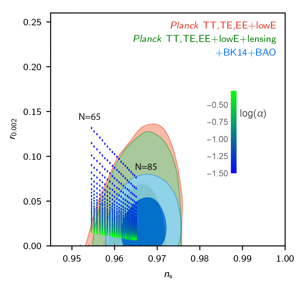
Figure 3: A plot of $r-n_{s}$. We assumed fixed values of $\lambda\sim 10^{-4}$ and $M_{P}=1$ and varied the $\alpha$ parameter, $\alpha\in(0.01,0.1)$. The number of e-folds represented in this figure are $65-85$.

Focusing on characteristic values for the parameters, namely $\alpha=0.1$, $\lambda=10^{-4}$, and $N\sim 75$, we obtain for the initial and final field values

$$\phi_{*}\sim 25M_{P}\quad \text{and}\quad\phi_{f}\sim 3M_{P},$$

or (3.10)

$$\zeta_{*}\sim 19M_{P}\quad \text{and}\quad\zeta_{f}\sim 3M_{P}.$$

At the same time the Lyth bound $|\Delta\phi|\gtrsim M_{P}\sqrt{r/4\pi}$ for this specific field excursion is trivially satisfied.

In Fig. 4, for the fixed value of ${{\alpha=0.1}}$ and $\lambda=10^{-4}$, we solve numerically the Klein-Gordon equation $\ddot{\zeta}+3H\dot{\zeta}+V^{\prime}(\zeta)=0$ for a plethora of initial conditions for the inflaton $\zeta$ and plot the trajectories in the $\zeta-\dot{\zeta}$ phase space. It is clear that the potential exhibits an attractor behaviour, since, regardless of initial conditions, all trajectories in phase space (green-dotted curves) quickly converge in a single trajectory that ends at the location of the potential minimum.

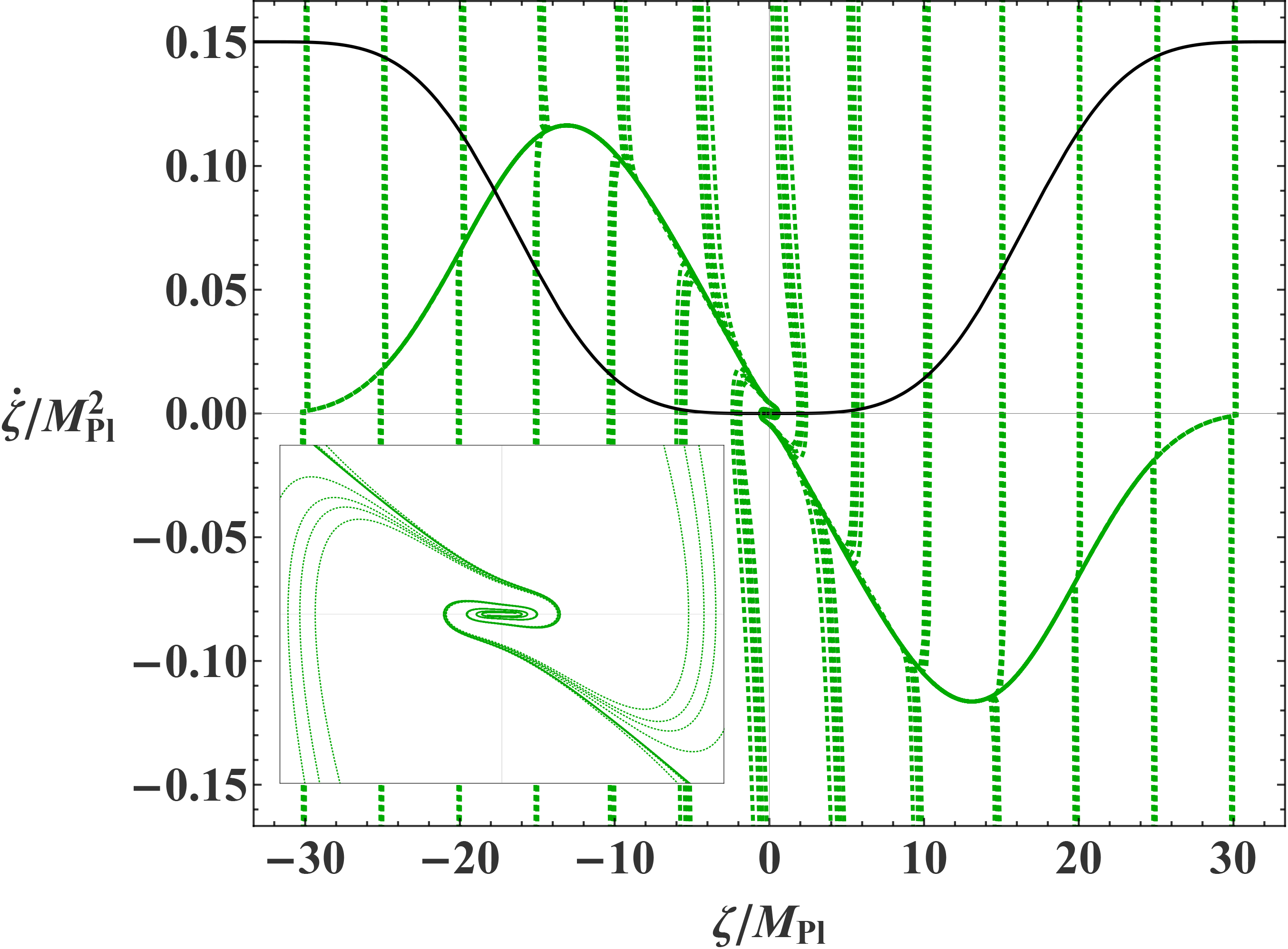
Figure 4: The attractor behaviour of the potential in the $\zeta-\dot{\zeta}$ phase space for $\alpha=0.1$ and $\lambda=10^{-4}$. A magnification of the region close to the minimum of the potential is also included in the bottom left. The black curve corresponds to the normalized potential.

3.2 Other Potentials

It has already been established that a quadratic potential in this Palatini framework leads to an acceptable inflationary behaviour. The quartic potential studied here is also supported by obvious particle physics renormalization and phenomenological arguments. This is not the case for potential functions with a large field behaviour carried out by a power greater than four. Nevertheless, it is interesting to analyze whether this behaviour is shared by more general functions, since for any increasing function $V(\phi)$ the effective potential $\bar{V}(\phi)=V(\phi)/\left(1+\frac{4\alpha}{M_{P}^{4}}V(\phi)\right)$ for large values of $\phi$ tends to a plateau $M_{P}^{4}/4\alpha$. As a general example we may consider a monomial potential $\lambda\phi^{2n}/4M_{P}^{2n-4}$. The case $n=1$ (quadratic potential) has been studied elsewhere [52] and is proven to exhibit acceptable inflationary behaviour. The integral defining the corresponding canonical field $\zeta$ can be estimated to behave as $C_{0}-C_{1}/x^{n-1}$ in terms of $x=(\alpha\lambda)^{\frac{1}{2n}}\phi/M_{P}$, following an analogous behaviour as in the quartic case. Similarly, the potential $\bar{V}=\frac{M_{P}^{4}}{4\alpha}\frac{x^{2n}}{1+x^{2n}}$ as a function of $\zeta$ follows the same behaviour reaching a plateau. The corresponding expressions for the slow-roll parameters are similar, being

$$\epsilon_{V}\,=\,\frac{2n^{2}(\alpha\lambda)^{\frac{1}{n}}}{x^{2}(1+x^{2n})},\qquad\eta_{V}\,=\,2n(\alpha\lambda)^{\frac{1}{n}}\frac{\left((2n-1)-(n+1)x^{2n}\right)}{x^{2}\left(1+x^{2n}\right)}\ .$$ (3.11)

The value of $x_{f}^{2}$ is obtained from $\epsilon_{V}(x_{f})\approx 1$. In the case that $2n^{2}(\alpha\lambda)^{1/n}$ is small this corresponds to $x_{f}^{2}\,\approx\,2n^{2}(\alpha\lambda)^{1/n}$. The number of e-folds is

$$N\,=\,\frac{1}{4n(\alpha\lambda)^{\frac{1}{n}}}\left(\,x_{*}^{2}\,-x_{f}^{2}\,\right)\ .$$ (3.12)

Focusing on the $n=3$ case with $\alpha\lambda\lesssim 10^{-2}$ we have $x_{f}^{2}\approx 18(\alpha\lambda)^{1/3}$. Substituting the expressions of $\epsilon_{V}$, $\eta_{V}$ for $n=3$ and $x_{*}^{2}=12(\alpha\lambda)^{1/3}(N+3/2)$, we obtain for the spectral index

$$n_{s}=\left.\frac{2N-(n+2)}{2N+n}\right|_{n=3}=\frac{2N-5}{2N+3}\ ,$$ (3.13)

which requires an unacceptably large number of e-folds in order to comply with the observed value of $n_{s}$. Therefore, the case $n=3$ is excluded for inflation. The same is true for larger values of $n$. Note however that for rational values of $n=q/p$ in the range $1<n<2$ the situation is different. For example $n=3/2$ leads to an acceptable value of $n_{s}$ for $N=55$. The same is true for $n=2/3$ and $n=4/3$, for $N\approx 50$ and $N\approx 65$ respectively.

General conclusions can also be drawn by taking the large $N$ limit of the above formula (3.13)

$$n_{s}=\frac{1-\frac{n+2}{2N}}{1+\frac{n}{2N}}\simeq 1-\frac{n+1}{N}\,,$$ (3.14)

which singles out the values of $n$ in the neighbourhood of $n=1$ (quadratic potential), as corresponding to the best fit value $n_{s}=1-2/N$.

4 Natural Inflation

As we saw in the preceding sections the main ingredient of the inflation mechanism operating in the Palatini framework for a model described by a potential $V(\phi)$ is the creation of a plateau for the Einstein-frame potential $\bar{V}(\phi)=V(\phi)/\left(1+4\alpha V(\phi)/M_{P}^{4}\right)$ at large field values. This mechanism works perfectly for quadratic and higgs-like quartic potentials leading to acceptable inflationary predictions, although it fails for steeper potential functions. On the other hand, it is possible for a model possessing an inflationary plateau in its standard metric formulation but falling short in its numerical predictions to yield improved results in the Palatini framework.

As an example, in what follows we consider the so-called natural inflation models, where the role of the inflaton is played by axions, i.e. pseudo-Nambu-Goldstone bosons arising whenever an approximate global symmetry is spontaneously broken [74, 75]. We assume a global shift symmetry of the inflaton field is spontaneously broken at some scale $f$, with soft explicit symmetry breaking at a lower scale $M$, which gives the boson its mass. The scalar potential is generally of the form

$$V(\phi)=M^{4}\left(1+\cos\left(\frac{\phi}{f}\right)\right)\ .$$ (4.1)

The potential has a height $2M^{4}$ and a unique minimum at $\phi=\pi f$, assuming the periodicity of $\phi$ is $2\pi f$. For appropriately chosen values of the mass scales, namely, $f\sim M_{P}$ and $M\sim M_{\rm GUT}$ the $\phi$ field can drive inflation. Nevertheless, the latest results from the Planck collaboration have excluded natural inflation [78, 79].

It is interesting to see how the predictions of natural inflation change in the Palatini framework with the $R^{2}$ term. The integral for the canonical field $\zeta$ yields

$$\zeta=\frac{2f}{1+2M^{4}}{\cal{F}}\left(\phi/2f,\,2M^{4}/(1+2M^{4})\right)\ ,$$ (4.2)

where ${\cal{F}}$ is again the elliptic integral of the first kind. The above expression can be easily inverted in terms of $\phi$. Then, the effective potential becomes

$$\bar{V}(\zeta)=\frac{2M^{4}\,{\rm cn}^{2}\left((1+2M^{4})^{1/2}\,\zeta/2f,\,2M^{4}/(1+2M^{4})\right)}{1+\frac{8\alpha M^{4}}{M^{4}_{P}}\,{\rm cn}^{2}\left((1+2M^{4})^{1/2}\,\zeta/2f,\,2M^{4}/(1+2M^{4})\right)}\ ,$$ (4.3)

with ${\rm cn}$ being the Jacobi elliptic function. Choosing $M=0.5$, $\alpha=10$, and $f=10$ (in natural units) we show in Fig. 5 the two potentials $V(\phi)$ and $\bar{V}(\zeta)$. For the chosen values of the parameters, one can see that the potential in the Palatini framework has a flatter plateau.

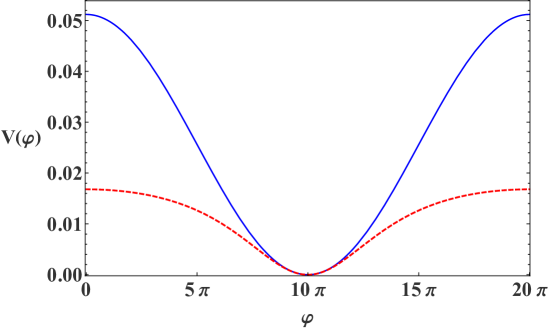
Figure 5: Blue curve: The original natural inflation potential $V(\phi)$. Red dashed curve: The potential $\bar{V}(\zeta(\phi))$ in the Palatini formalism. We have chosen $M=0.4$, $\alpha=10$, and $f=10$ (in natural units).

Next, we proceed with the calculation of the inflationary observables. We assume slow-roll conditions for the canonically normalized field $\zeta$ and follow a similar line of analysis, as in the previous section. In the following figure we present the $r$-$n_{s}$ predictions, plotted against the Planck 2018 $1\sigma$ and $2\sigma$ curves [79].

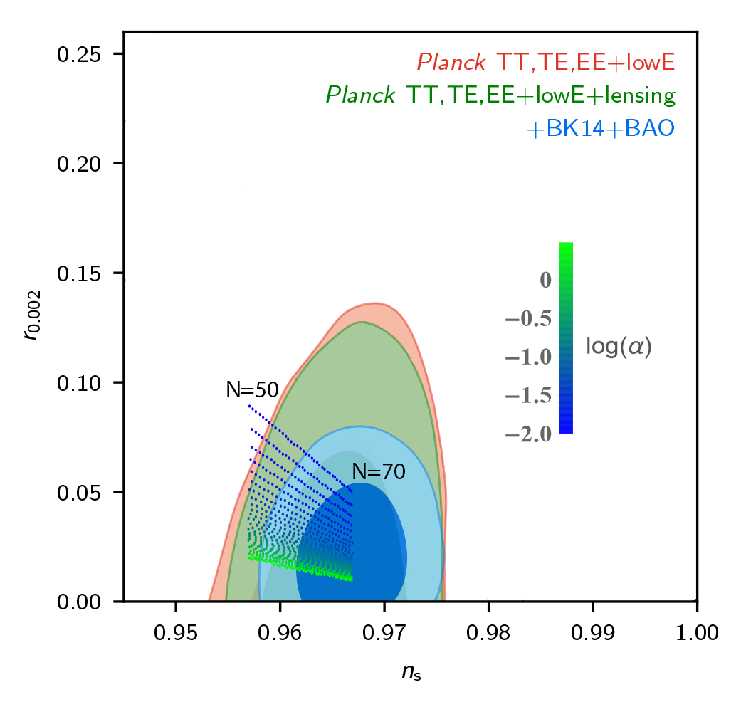
Figure 6: $r-n_{s}$ plot for $M=0.7,f=7$ and $\alpha\in[0.01,3]$ in natural units.

For a specific set of the scale parameters $(M,f)$, the variation of $\alpha$ only affects the tensor-to-scalar ratio $r$. By increasing $\alpha$ we obtain smaller values of $r$. There is a lower bound on the scale $f\gtrsim 7$ (in natural units), set by the Planck collaboration [78], to which we also abide by here. Increasing the scale $f$ results in pushing the curve to larger values of $r$ and $n_{s}$.

In Fig. 7, for the value of ${{\alpha=10}}$ and $f=10$ (the period is $2\pi$), we solve numerically the Klein-Gordon equation $\ddot{\zeta}+3H\dot{\zeta}+\bar{V}^{\prime}(\zeta)=0$ for a plethora of initial conditions for the inflaton $\zeta$ and plot the trajectories in $\zeta-\dot{\zeta}$ phase space, showing the attractor behaviour of the potential.

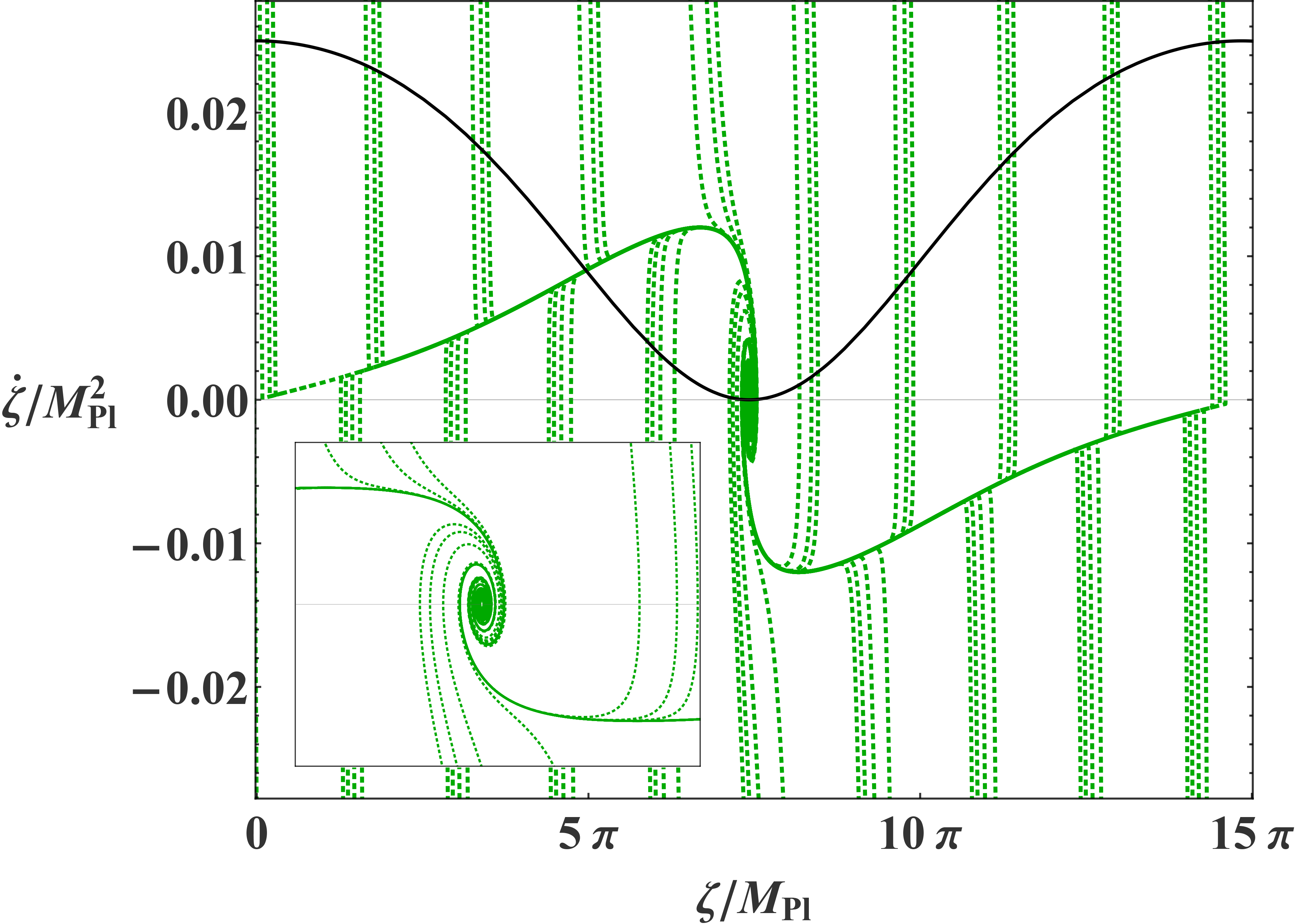
Figure 7: The attractor behaviour of the potential in the $\zeta-\dot{\zeta}$ phase space for $M=0.4,\alpha=0.01-3$ and $f=7$. A magnification of the region close to the minimum of the potential is also included in the bottom left. The black curve corresponds to the normalized potential.

5 Summary and Conclusions

In this article we considered scalar fields coupled to gravity in the framework of the Palatini formalism. We focused on the case that the theory, extended with a quadratic curvature term $R/2+\alpha R^{2}/4$ (rewritten in terms of an auxiliary scalar as $(1+\alpha\chi^{2})R/2-\chi^{4}/4$), also includes fundamental scalar fields coupled minimally to gravity and self-interacting through a scalar potential $V(\phi)$. Transforming the theory to the Einstein frame and integrating out the auxiliary non-propagating scalar degree of freedom we end up with an Einstein frame scalar potential of the form $\overline{V}(\phi)=V(\phi)/\left(1+4\alpha\,V(\phi)\right)$ which, under general conditions, could in principle lead to an inflationary plateau for large field values, this property being a central feature of this framework.

We analyzed the slow-roll inflationary behaviour in the case of a quartic potential and found acceptable inflationary predictions for the spectral index and tensor to scalar ratio. This case could be of interest for realizing Higgs inflation with a minimal coupling to gravity. We also considered other monomial potentials, although the analogous inflationary behaviour is not shared by steeper potential functions. Next, we analyzed the case of the natural inflation or cosine inflation model, where the role of the inflaton is undertaken by a pseudo-Goldstone boson (axion). Although these models, characterized by a bounded periodic potential, fall short in their inflationary predictions in the standard formulation, when considered in the presence of an $R^{2}$ term in the framework of the Palatini formalism are shown to yield quite acceptable values for the inflationary observables.

References

- [1] A. A. Starobinsky, A New Type of Isotropic Cosmological Models Without Singularity, Phys. Lett. 91B (1980) 99–102.
- [2] K. Sato, First Order Phase Transition of a Vacuum and Expansion of the Universe, Mon. Not. Roy. Astron. Soc. 195 (1981) 467–479.
- [3] A. H. Guth, The Inflationary Universe: A Possible Solution to the Horizon and Flatness Problems, Phys. Rev. D23 (1981) 347–356.
- [4] A. D. Linde, A New Inflationary Universe Scenario: A Possible Solution of the Horizon, Flatness, Homogeneity, Isotropy and Primordial Monopole Problems, Phys. Lett. 108B (1982) 389–393. [Adv. Ser. Astrophys. Cosmol.3,149(1987)].
- [5] A. Albrecht and P. J. Steinhardt, Cosmology for Grand Unified Theories with Radiatively Induced Symmetry Breaking, Phys. Rev. Lett. 48 (1982) 1220–1223. [Adv. Ser. Astrophys. Cosmol.3,158(1987)].
- [6] A. D. Linde, Chaotic Inflation, Phys. Lett. 129B (1983) 177–181.
- [7] D. H. Lyth and A. Riotto, Particle physics models of inflation and the cosmological density perturbation, Physics Reports 314 (1999), no. 1 1–146.
- [8] A. De Simone, M. P. Hertzberg, and F. Wilczek, Running Inflation in the Standard Model, Phys. Lett. B678 (2009) 1–8, [arXiv:0812.4946].
- [9] J. L. F. Barbon and J. R. Espinosa, On the Naturalness of Higgs Inflation, Phys. Rev. D79 (2009) 081302, [arXiv:0903.0355].
- [10] F. L. Bezrukov and M. Shaposhnikov, The Standard Model Higgs boson as the inflaton, Phys. Lett. B659 (2008) 703–706, [arXiv:0710.3755].
- [11] A. O. Barvinsky, A. Yu. Kamenshchik, and A. A. Starobinsky, Inflation scenario via the Standard Model Higgs boson and LHC, JCAP 0811 (2008) 021, [arXiv:0809.2104].
- [12] A. O. Barvinsky, A. Yu. Kamenshchik, C. Kiefer, A. A. Starobinsky, and C. Steinwachs, Asymptotic freedom in inflationary cosmology with a non-minimally coupled Higgs field, JCAP 0912 (2009) 003, [arXiv:0904.1698].
- [13] F. L. Bezrukov, A. Magnin, and M. Shaposhnikov, Standard Model Higgs boson mass from inflation, Phys. Lett. B675 (2009) 88–92, [arXiv:0812.4950].
- [14] R. N. Lerner and J. McDonald, A Unitarity-Conserving Higgs Inflation Model, Phys. Rev. D82 (2010) 103525, [arXiv:1005.2978].
- [15] F. Bezrukov, A. Magnin, M. Shaposhnikov, and S. Sibiryakov, Higgs inflation: consistency and generalisations, JHEP 01 (2011) 016, [arXiv:1008.5157].
- [16] K. Kamada, T. Kobayashi, T. Takahashi, M. Yamaguchi, and J. Yokoyama, Generalized Higgs inflation, Phys. Rev. D86 (2012) 023504, [arXiv:1203.4059].
- [17] F. Bezrukov, The Higgs field as an inflaton, Class. Quant. Grav. 30 (2013) 214001, [arXiv:1307.0708].
- [18] Y. Hamada, H. Kawai, and K.-y. Oda, Minimal Higgs inflation, PTEP 2014 (2014) 023B02, [arXiv:1308.6651].
- [19] F. Bezrukov and M. Shaposhnikov, Higgs inflation at the critical point, Phys. Lett. B734 (2014) 249–254, [arXiv:1403.6078].
- [20] K. Allison, Higgs xi-inflation for the 125-126 GeV Higgs: a two-loop analysis, JHEP 02 (2014) 040, [arXiv:1306.6931].
- [21] A. Salvio and A. Mazumdar, Classical and Quantum Initial Conditions for Higgs Inflation, Phys. Lett. B750 (2015) 194–200, [arXiv:1506.07520].
- [22] Y. Hamada, H. Kawai, K.-y. Oda, and S. C. Park, Higgs inflation from Standard Model criticality, Phys. Rev. D91 (2015) 053008, [arXiv:1408.4864].
- [23] X. Calmet and I. Kuntz, Higgs Starobinsky Inflation, Eur. Phys. J. C76 (2016), no. 5 289, [arXiv:1605.02236].
- [24] J. Rubio, Higgs inflation, arXiv:1807.02376.
- [25] V.-M. Enckell, K. Enqvist, S. Rasanen, and E. Tomberg, Higgs inflation at the hilltop, JCAP 1806 (2018), no. 06 005, [arXiv:1802.09299].
- [26] H. Weyl, A Remark on the coupling of gravitation and electron, Phys. Rev. 77 (1950) 699–701.
- [27] S. Deser and C. J. Isham, Canonical Vierbein Form of General Relativity, Phys. Rev. D14 (1976) 2505.
- [28] F. W. Hehl, J. D. McCrea, E. W. Mielke, and Y. Ne’eman, Metric affine gauge theory of gravity: Field equations, Noether identities, world spinors, and breaking of dilation invariance, Phys. Rept. 258 (1995) 1–171, [gr-qc/9402012].
- [29] S. Deser, First-order formalism and odd-derivative actions, Class. Quant. Grav. 23 (2006) 5773, [gr-qc/0606006].
- [30] F. Bauer and D. A. Demir, Inflation with Non-Minimal Coupling: Metric versus Palatini Formulations, Phys. Lett. B665 (2008) 222–226, [arXiv:0803.2664].
- [31] T. P. Sotiriou and V. Faraoni, f(R) Theories Of Gravity, Rev. Mod. Phys. 82 (2010) 451–497, [arXiv:0805.1726].
- [32] M. Borunda, B. Janssen, and M. Bastero-Gil, Palatini versus metric formulation in higher curvature gravity, JCAP 0811 (2008) 008, [arXiv:0804.4440].
- [33] G. J. Olmo, Palatini Approach to Modified Gravity: f(R) Theories and Beyond, Int. J. Mod. Phys. D20 (2011) 413–462, [arXiv:1101.3864].
- [34] F. Bauer and D. A. Demir, Higgs-Palatini Inflation and Unitarity, Phys. Lett. B698 (2011) 425–429, [arXiv:1012.2900].
- [35] N. Tamanini and C. R. Contaldi, Inflationary Perturbations in Palatini Generalised Gravity, Phys. Rev. D83 (2011) 044018, [arXiv:1010.0689].
- [36] K. Enqvist, T. Koivisto, and G. Rigopoulos, Non-metric chaotic inflation, JCAP 1205 (2012) 023, [arXiv:1107.3739].
- [37] A. Borowiec, M. Kamionka, A. Kurek, and M. Szydlowski, Cosmic acceleration from modified gravity with Palatini formalism, JCAP 1202 (2012) 027, [arXiv:1109.3420].
- [38] A. Racioppi, Coleman-Weinberg linear inflation: metric vs. Palatini formulation, JCAP 1712 (2017), no. 12 041, [arXiv:1710.04853].
- [39] S. Rasanen and P. Wahlman, Higgs inflation with loop corrections in the Palatini formulation, JCAP 1711 (2017), no. 11 047, [arXiv:1709.07853].
- [40] C. Fu, P. Wu, and H. Yu, Inflationary dynamics and preheating of the nonminimally coupled inflaton field in the metric and Palatini formalisms, Phys. Rev. D96 (2017), no. 10 103542, [arXiv:1801.04089].
- [41] A. Stachowski, M. Szydłowski, and A. Borowiec, Starobinsky cosmological model in Palatini formalism, Eur. Phys. J. C77 (2017), no. 6 406, [arXiv:1608.03196].
- [42] M. Szydłowski, A. Stachowski, and A. Borowiec, Emergence of running dark energy from polynomial f(R) theory in Palatini formalism, Eur. Phys. J. C77 (2017), no. 9 603, [arXiv:1707.01948].
- [43] T. Tenkanen, Resurrecting Quadratic Inflation with a non-minimal coupling to gravity, JCAP 1712 (2017), no. 12 001, [arXiv:1710.02758].
- [44] T. Markkanen, T. Tenkanen, V. Vaskonen, and H. Veermäe, Quantum corrections to quartic inflation with a non-minimal coupling: metric vs. Palatini, JCAP 1803 (2018), no. 03 029, [arXiv:1712.04874].
- [45] P. Carrilho, D. Mulryne, J. Ronayne, and T. Tenkanen, Attractor Behaviour in Multifield Inflation, JCAP 1806 (2018), no. 06 032, [arXiv:1804.10489].
- [46] V.-M. Enckell, K. Enqvist, S. Rasanen, and L.-P. Wahlman, Inflation with term in the Palatini formalism, arXiv:1810.05536.
- [47] A. Kozak and A. Borowiec, Palatini frames in scalar-tensor theories of gravity, arXiv:1808.05598.
- [48] L. Järv, A. Racioppi, and T. Tenkanen, Palatini side of inflationary attractors, Phys. Rev. D97 (2018), no. 8 083513, [arXiv:1712.08471].
- [49] Z. Wang, P. Wu, and H. Yu, Stability analysis for non-minimally coupled dark energy models in the Palatini formalism, Astrophys. Space Sci. 363 (2018), no. 6 120.
- [50] J. Wu, G. Li, T. Harko, and S.-D. Liang, Palatini formulation of gravity theory, and its cosmological implications, Eur. Phys. J. C78 (2018), no. 5 430, [arXiv:1805.07419].
- [51] M. Szydłowski and A. Stachowski, Polynomial Palatini cosmology – dynamical system approach, Phys. Rev. D97 (2018), no. 10 103524, [arXiv:1712.00822].
- [52] I. Antoniadis, A. Karam, A. Lykkas, and K. Tamvakis, Palatini inflation in models with an term, JCAP 1811 (2018), no. 11 028, [arXiv:1810.10418].
- [53] S. Rasanen and E. Tomberg, Planck scale black hole dark matter from Higgs inflation, arXiv:1810.12608.
- [54] S. Rasanen, Higgs inflation in the Palatini formulation with kinetic terms for the metric, arXiv:1811.09514.
- [55] J. P. B. Almeida, N. Bernal, J. Rubio, and T. Tenkanen, Hidden Inflaton Dark Matter, arXiv:1811.09640.
- [56] V. H. Cardenas, S. del Campo, and R. Herrera, R**2 corrections to chaotic inflation, Mod. Phys. Lett. A18 (2003) 2039–2050, [gr-qc/0308040].
- [57] M. Artymowski, Z. Lalak, and M. Lewicki, Inflationary scenarios in Starobinsky model with higher order corrections, JCAP 1506 (2015) 032, [arXiv:1502.01371].
- [58] C. van de Bruck and L. E. Paduraru, Simplest extension of Starobinsky inflation, Phys. Rev. D92 (2015) 083513, [arXiv:1505.01727].
- [59] T. Asaka, S. Iso, H. Kawai, K. Kohri, T. Noumi, and T. Terada, Reinterpretation of the Starobinsky model, PTEP 2016 (2016), no. 12 123E01, [arXiv:1507.04344].
- [60] M. Artymowski, Z. Lalak, and M. Lewicki, Saddle point inflation from higher order corrections to Higgs/Starobinsky inflation, Phys. Rev. D93 (2016), no. 4 043514, [arXiv:1509.00031].
- [61] S. Kaneda and S. V. Ketov, Starobinsky-like two-field inflation, Eur. Phys. J. C76 (2016), no. 1 26, [arXiv:1510.03524].
- [62] C. van de Bruck, P. Dunsby, and L. E. Paduraru, Reheating and preheating in the simplest extension of Starobinsky inflation, arXiv:1606.04346.
- [63] Y.-C. Wang and T. Wang, Primordial perturbations generated by Higgs field and operator, Phys. Rev. D96 (2017), no. 12 123506, [arXiv:1701.06636].
- [64] Y. Ema, Higgs Scalaron Mixed Inflation, Phys. Lett. B770 (2017) 403–411, [arXiv:1701.07665].
- [65] T. Mori, K. Kohri, and J. White, Multi-field effects in a simple extension of inflation, JCAP 1710 (2017), no. 10 044, [arXiv:1705.05638].
- [66] S. Pi, Y.-l. Zhang, Q.-G. Huang, and M. Sasaki, Scalaron from -gravity as a heavy field, JCAP 1805 (2018), no. 05 042, [arXiv:1712.09896].
- [67] M. He, A. A. Starobinsky, and J. Yokoyama, Inflation in the mixed Higgs- model, JCAP 1805 (2018), no. 05 064, [arXiv:1804.00409].
- [68] D. Gorbunov and A. Tokareva, Scalaron the healer: removing the strong-coupling in the Higgs- and Higgs-dilaton inflations, arXiv:1807.02392.
- [69] D. M. Ghilencea, Two-loop corrections to Starobinsky-Higgs inflation, arXiv:1807.06900.
- [70] S.-J. Wang, Quintessential Starobinsky inflation and swampland criteria, arXiv:1810.06445.
- [71] F. Bombacigno and G. Montani, Cosmological implementation of Palatini models with a Nieh-Yan term, arXiv:1809.07563.
- [72] A. Gundhi and C. F. Steinwachs, Scalaron-Higgs inflation, arXiv:1810.10546.
- [73] A. Karam, T. Pappas, and K. Tamvakis, Nonminimal Coleman–Weinberg Inflation with an term, arXiv:1810.12884.
- [74] K. Freese, J. A. Frieman, and A. V. Olinto, Natural inflation with pseudo - Nambu-Goldstone bosons, Phys. Rev. Lett. 65 (1990) 3233–3236.
- [75] F. C. Adams, J. R. Bond, K. Freese, J. A. Frieman, and A. V. Olinto, Natural inflation: Particle physics models, power law spectra for large scale structure, and constraints from COBE, Phys. Rev. D47 (1993) 426–455, [hep-ph/9207245].
- [76] R. Z. Ferreira and A. Notari, Thermalized axion inflation: natural and monomial inflation with small , Phys. Rev. D97 (2018), no. 6 063528, [arXiv:1711.07483].
- [77] R. Z. Ferreira, A. Notari, and G. Simeon, Natural Inflation with a periodic non-minimal coupling, JCAP 1811 (2018), no. 11 021, [arXiv:1806.05511].
- [78] Planck Collaboration, P. A. R. Ade et al., Planck 2015 results. XX. Constraints on inflation, Astron. Astrophys. 594 (2016) A20, [arXiv:1502.02114].
- [79] Planck Collaboration, Y. Akrami et al., Planck 2018 results. X. Constraints on inflation, arXiv:1807.06211.