Characterization and history of the Helmi streams with Gaia DR2

Abstract

Context. The halo of the Milky Way has long been hypothesized to harbour significant amounts of merger debris. This view has been supported over more than a decade by wide-field photometric surveys which have revealed the outer halo to be lumpy.

Aims. The recent release of Gaia DR2 is allowing us to establish that mergers also have been important and possibly built up the majority of the inner halo. In this work we focus on the Helmi streams, a group of streams crossing the Solar vicinity and known for almost two decades. We characterize their properties and relevance for the build-up of the Milky Way’s halo.

Methods. We identify new members of the Helmi streams in an unprecedented dataset with full phase-space information combining Gaia DR2, and the APOGEE DR2, RAVE DR5 and LAMOST DR4 spectroscopic surveys. Based on the orbital properties of the stars, we find new stream members up to a distance of 5 kpc from the Sun, which we characterize using photometry and metallicity information. We also perform N-body experiments to constrain the time of accretion and properties of the progenitor of the streams.

Results. We find nearly 600 new members of the Helmi streams. Their HR diagram reveals a broad age range, from approximately 11 to 13 Gyr, while their metallicity distribution goes from $-2.3$ to $-1.0$, and peaks at [Fe/H] $\sim-1.5$. These findings confirm that the streams originate in a dwarf galaxy. Furthermore, we find 7 globular clusters to be likely associated, and which follow a well-defined age-metallicity sequence whose properties suggest a relatively massive progenitor object. Our N-body simulations favour a system with a stellar mass of $\sim 10^{8}\,\mathrm{M}_{\odot}$ accreted $5-8$ Gyr ago.

Conclusions. The debris from the Helmi streams is an important donor to the Milky Way halo, contributing approximately 15% of its mass in field stars and 10% of its globular clusters.

1 Introduction

According to the concordance cosmological model $\Lambda$CDM, galaxies grow by mass through mergers. Typically a galaxy’s halo is formed through a handful of major mergers accompanied by a plethora of minor mergers. This model’s predictions stem both from dark matter only simulations (Helmi et al., 2003) combined with semi-analytic models of galaxy formation (e.g. Bullock & Johnston, 2005; Cooper et al., 2010) and hydrodynamical simulations (e.g. Pillepich et al., 2014).

When satellites merge with a galaxy like the Milky Way they get stripped of their stars by the tidal forces, e.g. Johnston et al. (1996). These stars follow approximately the mean orbit of their progenitor and this leads to the formation of streams and shells. Wide-field photometric surveys have already discovered many cold streams likely due to globular clusters, e.g. Pal 5 (Odenkirchen et al., 2001); GD-1 (Grillmair & Dionatos, 2006), and more disperse streams caused by dwarf galaxies, e.g. Sagittarius (Ibata et al., 1994), as well as large overdensities such as those visible in the SDSS or Pan-STARRS maps (Belokurov et al., 2006; Bernard et al., 2016). Many of these streams are distant and have become apparent after meticulous filtering (e.g. Rockosi et al., 2002; Grillmair, 2009).

Tidal debris in the vicinity of the Sun is predicted to be very phase-mixed (Helmi & White, 1999; Helmi et al., 2003). Typically one can expect to find many stream wraps originating in the same object, i.e. groups of stars with different orbital phase sharing a common origin. Because of the high degree of phase-mixing, it is more productive to study tidal debris in spaces such as those defined by the velocities, integrals of motion (Helmi & de Zeeuw, 2000), or in action space (Mcmillan & Binney, 2008), rather than to search for clustering in spatial coordinates. Until recently, a few studies on the nearby stellar halo identified different small groups of stars that likely were accreted together, e.g. Helmi et al. (1999); Chiba & Beers (2000); Helmi et al. (2006); Klement et al. (2008, 2009); Majewski et al. (2012); Beers et al. (2017); Helmi et al. (2017), see Newberg & Carlin (2016) for a comprehensive review.

A new era is dawning now that the Gaia mission is delivering full phase-space information for a billion stars. As it is clear from the above discussion, this is crucial to unravel the merger history of the Milky Way and to characterize the properties its progenitors. In fact, the second data release of the Gaia mission (Gaia Collaboration, Brown et al., 2018) is already transforming the field of galactic archaeology.

The strength of Gaia, and especially of the 6D sample, is that it can identify stream members based on the measured kinematics (e.g. Koppelman et al., 2018; Price-Whelan & Bonaca, 2018). Arguably the most recent spectacular finding possible thanks to Gaia is the discovery that the inner halo was built largely via the accretion of a single object, as first hinted from the kinematics (Belokurov et al., 2018; Koppelman et al., 2018), and the stellar populations (Gaia Collaboration, Babusiaux et al., 2018; Haywood et al., 2018), all pieces put together in Helmi et al. (2018). This accreted system known as Gaia-Enceladus was disky and similar in mass to the Small Magellanic Cloud today, and hence led to the heating of a proto-disk some 10 Gyr ago (Helmi et al., 2018).

Gaia-Enceladus debris however, is not the only substructure present in the vicinity of the Sun. Detected about 20 years ago, the Helmi streams (Helmi et al., 1999, H99 hereafter) are known to cross the Solar neighbourhood. Their existence has been confirmed by Chiba & Beers (2000) and Smith et al. (2009), among other studies. In the original work, 13 stars were detected based on their clumped angular momenta which clearly differ from other local halo stars. Follow-up work by Kepley et al. (2007) estimated that the streams were part of the tidal debris of a dwarf galaxy that was accreted $6-9$ Gyr ago, based on the bimodality of the $z$-velocity distribution. This bimodal distribution is the distinctive feature of multiple wraps of tidal debris crossing the Solar neighbourhood. Since the discovery in 1999, a handful of new tentative members have been found increasing the total number of members to $\sim 30$ (e.g. Kepley et al., 2007; Re Fiorentin et al., 2005; Klement et al., 2009; Beers et al., 2017), while several tens more were reported in Gaia Collaboration, Helmi et al. (2018). Also structure S2 from Myeong et al. (2018a), consisting of $\sim 60$ stars, has been recognized to be related to the Helmi streams .

Originally, the Helmi streams were found using Hipparcos proper motions (Perryman et al., 1997) combined with ground-based radial velocities (Beers & Sommer-Larsen, 1995; Chiba & Yoshii, 1998). In this work, we aim to find new members and to characterize better its progenitor in terms of the time of accretion, initial mass and star formation history. To this end we focus on the dynamics, metallicity distribution and colour-magnitude diagram of its members. Furthermore, we also identify globular clusters that could have potentially been accreted with the object (Leaman et al., 2013; Kruijssen et al., 2018), as for example seen for the Sagittarius dwarf galaxy (Law & Majewski, 2010; Massari et al., 2017; Sohn et al., 2018), and also for Gaia-Enceladus (Myeong et al., 2018b; Helmi et al., 2018).

This paper is structured as follows: in Section 2 we present the data and samples used, while in Section 3 we define a core selection of streams members that serves as the basis to identify more members. In Section 4 we analyze the spatial distribution of the debris. In Section 5 we supplement the observations with N-body simulations. We discuss possible associations of the Helmi streams with globular clusters in Section 6. Finally, we present our conclusions in Section 7.

2 Data

2.1 Brief description of the data

The recently published second data release (DR2) of the Gaia space mission contains the on-sky positions, parallaxes, proper motions, and the $G$, $G_{\mathrm{BP}}$ and $G_{\mathrm{RP}}$ optical magnitudes for over 1.3 billion stellar sources in the Milky Way (Gaia Collaboration, Brown et al., 2018). For 7,224,631 stars with $G_{\mathrm{RVS}}$ ¡ 12, known as the 6D subsample, line-of-sight velocity information measured by the Gaia satellite is available (Gaia Collaboration, Katz et al., 2018). The precision of the observables in this dataset are unprecedented: the median proper motions uncertainties of the stars with full phase-space information, is 1.5 mas/yr which translates to a tangential velocity error of $\sim 7$ km/s for a star at 1 kpc, while their median radial velocity uncertainties are 3.3 km/s. This makes the Gaia DR2 both the highest quality and the largest size single survey ever available for studying the kinematics and dynamics of the nearby stellar halo and disk.

2.2 Cross-matching with APOGEE, RAVE and LAMOST

To supplement the 6D Gaia subsample, we add the radial velocities from the cross-matched catalogues APOGEE (Wilson et al., 2010; Abolfathi et al., 2018) and RAVE DR5 (Kunder et al., 2017), see Marrese et al. (2018) for details. We also add radial velocities from our own cross-match of Gaia DR2 with LAMOST DR4 (Cui et al., 2012).

For the cross-match with LAMOST we first transform the stars to the same reference frame using the Gaia positions and proper motions, and then we match stars within a radius of 10 arcsec with TOPCAT/STILTS (Taylor, 2005, 2006). We find that over 95% of the stars have a matching radius smaller than 0.5 arcsec. In total, we find 2,868,425 matches between Gaia and LAMOST DR4, with a subset of 8,404 overlapping also with RAVE, and 50,650 with APOGEE. Because the LAMOST radial velocities are known to be offset by $+4.5$ km/s with respect to APOGEE (Anguiano et al., 2018), we correct for this effect.

Since the radial velocities of RAVE and APOGEE have been shown to be very consistent with those of Gaia (Sartoretti et al., 2018), for our final catalogue, we use first the radial velocities from APOGEE if available, then those from RAVE, and finally from LAMOST for the stars for which there is no overlap with either two of the other surveys. After imposing a quality cut of parallax_over_error $>5$, this yields a sample of 2,361,519 stars with radial velocities. Note that all these surveys also provide additional metallicity information for a subset of the stars.

When combined with the Gaia 6D sample, this results in a total of 8,738,322 stars with 6D information and parallax_over_error $>5$. The median line-of-sight velocity error of the stars from the ground-based spectroscopic surveys is 5.8 km/s, while that of the pure Gaia sample is 1 km/s for the same parallax quality cut.

2.3 Quality cuts and halo selection

To isolate halo stars, we follow a kinematic selection, i.e. stars are selected because of their very different velocity from local disk stars. By cutting in velocity we introduce a clear bias: halo stars with disk-like kinematics are excluded from this sample (Nissen & Schuster, 2010; Bonaca et al., 2017; Posti et al., 2018; Koppelman et al., 2018). Nevertheless, the amplitude of the $Z$-velocities of the Helmi streams stars is $>200$ km/s, i.e. very different from the disk, so our selection should not impact our ability to find more members.

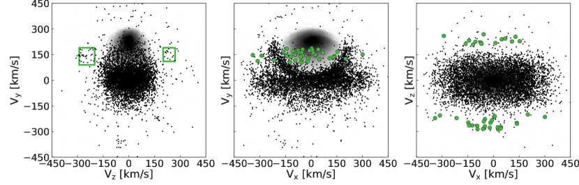
Figure 1: Velocity distribution of kinematically selected halo stars (black dots) within 1 kpc from the Sun from the Gaia-only 6D sample. The grey density in the background shows the location and extent of the disk in this diagram. The velocities have been corrected for the motion of the Sun and LSR. The green boxes in the left panel indicate the location of the Helmi streams, and are drawn based on the velocities of the original stream members. The stars inside these boxes are highlighted with green symbols in the other two panels.

We start from our extended 6D data sample (obtained as described in the previous section), and remove stars with parallax_over_error ¿ 5. Because of the zero-point offset of $\sim-0.03$ mas known to affect the Gaia parallaxes (Arenou et al., 2018; Gaia Collaboration, Brown et al., 2018; Lindegren et al., 2018) we also discard stars with parallaxes ¡ 0.2 mas. Distances for this reduced sample are obtained by inverting the parallaxes. Finally, following Koppelman et al. (2018) we select stars that have $|\boldsymbol{V}-\boldsymbol{V_{\mathrm{LSR}}}|>210$ km/s, where $\boldsymbol{V_{\mathrm{LSR}}}$ is the velocity vector of the local standard of rest (LSR). This cut is not too strict, allowing for some contamination from the thick disk. This velocity selection is done after correcting for the motion of the Sun using the values from Schönrich et al. (2010) and that of the LSR as estimated by Mcmillan (2017). Our Cartesian reference frame is pointed such that $X$ is positive toward the Galactic Centre, $Y$ points in the direction of the motion of the disk, and $Z$ is positive for Galactic latitude $b>0$. This final sample contains 79,318 tentative halo stars, with 12,472 located within 1 kpc from the Sun, which is at 8.2 kpc from the Galactic Centre (Mcmillan, 2017). Slightly more than half of these stars stem from the Gaia-only 6D sample.

3 Finding members

3.1 Core selection

Using the halo sample described above, we will select ‘core members’ by considering only those stars within 1 kpc from the Sun from the Gaia-only sample. In such a local sample, streams are very clustered in velocity-space because the gradients caused by the orbital motion are minimized.

Fig. 1 shows with green boxes our selection of the streams’ core members in velocity space. The boxes are placed on top of the positions of the original members of the Helmi streams. The boundaries in $(V_{Z},V_{Y})$ for the left box are: $[-290,-200]\,[90,190]$ km/s, and for the right box: $[200,270]\,[110,190]$ km/s. Using the SIMBAD database we find that 10 of the original 13 members have Gaia DR2 distances smaller than $1$ kpc. Of these 10 stars, 9 have radial velocities in our extended data sample. Only one star with updated radial velocity information has very different velocities, leaving the original sample with 8 reliable members with full Gaia 6D parameters within $1$ kpc.

One of the key characteristics of the Helmi streams are the two groups in the $V_{Y}-V_{Z}$ plane, one moving up through the disk and one moving down. Using the selection described above we find 40 core members in the Gaia-only sample, of which 26 with $V_{Z}<0$. The asymmetry in the number of stars in the two streams can be used as an indicator of the time of accretion and/or mass of the progenitor since tidal streams will only produce multiple wraps locally after having evolved for a sufficiently long time. In §5.1 we explore what the observed asymmetry implies for the properties of the progenitor of the Helmi streams.

Table 1: Gaia DR2 source_id of the Helmi streams’ core members.

IDs members 1-20	IDs members 21-40
365903386527108864	604095572614068352
640225833940128256	1049376272667191552
1415635209471360256	1621470761217916800
1639946061258413312	2075971480449027840
2081319509311902336	2268048503896398720
2322233192826733184	2416023871138662784
2447968154259005952	2556488440091507584
2604228169817599104	2670534149811033088
2685833132557398656	2891152566675457280
3085891537839264896	3085891537839267328
3202308378739431936	3214420461393486208
3306026508883214080	3742101345970116224
4440446153372208640	4768015406298936960
4998741805354135552	5032050552340352384
5049085217270417152	5388612346343578112
5558256888748624256	5986385619765488384
6050982889930146304	6170808423037019904
6221846137890957312	6322846447087671680
6336613092877645440	6545771884159036928
6615661065172699776	6914409197757803008

3.2 Beyond the core selection

The original 13 H99 members are located within 2.5 kpc from the Sun. Beyond this distance, we expect that other members of the streams will have different kinematic properties because of velocity gradients along their orbit. Therefore the best way of finding more members beyond the local volume is to use integrals of motion (IOM) such as angular momenta and energy or the action integrals (Helmi & de Zeeuw, 2000). Note that from this section onwards, we use the extended sample described in Section 2.2 and which includes radial velocities from APOGEE/RAVE/LAMOST.

Here we will mainly base the membership selection on the angular momentum of the stars, namely the $z$-component $L_{z}$, and the perpendicular component: $L_{\perp}=\sqrt{L_{x}^{2}+L_{y}^{2}}$, although the latter is generally not fully conserved. Since the energy $E$ depends on the assumed model for the galactic potential, we use it only to check for outliers.

To calculate the energy of the stars we model the Milky Way with a potential that is similar to that used by Helmi et al. (2017): it includes a Miyamoto-Nagai disk with parameters $\mathrm{M}_{d}=9.3\cdot 10^{10}\,\mathrm{M}_{\odot}$, $(a_{d},b_{d})=(6.5,0.26)\,\mathrm{kpc}$, an NFW halo with parameters $\mathrm{M}_{h}=10^{12}\,\mathrm{M}_{\odot}$, $r_{s,h}=21.5\,\mathrm{kpc}$, $c_{h}=12$, and a Hernquist bulge with parameters $\mathrm{M}_{b}=3\cdot 10^{10}\,\mathrm{M}_{\odot}$, $c_{b}=0.7$ kpc. The circular velocity curve of this potential is similar to that of the Milky Way. Since this potential is axisymmetric $L_{z}$ is a true IOM. Note that for convenience, in what follows we flip the sign of $L_{z}$ such that it is positive for the Sun.

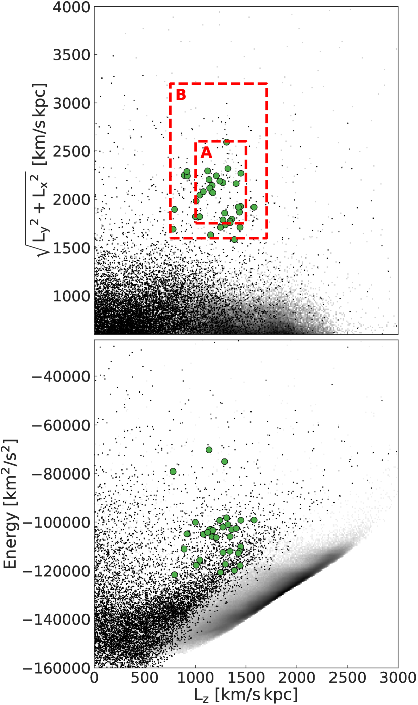
Figure 2: Distribution of the core members of the Helmi streams (green symbols), in angular momentum $L_{\perp}$ and $L_{z}$ in the top panel, and energy $E$ and $L_{z}$ in the bottom panel. The black dots show all of the stars of our sample of kinematically selected halo stars, located within 2.5 kpc from the Sun. With red, dashed lines we indicate the limits we apply to select additional members of the Helmi streams. In the background, the location of the disk(s) is shown with a grey density map.

In Fig. 2 we show the distribution of the core members in $L_{z}$ versus $L_{\perp}$ (top), and $L_{z}$ versus $E$ (bottom). A grey density map of all the stars in the Gaia 6D sample with 20% relative parallax error and with parallax $>0.2$ illustrates the location of the disk. The black dots correspond to all kinematically selected halo stars within 2.5 kpc from the Sun. The transition of the halo into the disk is smooth, and only appears sharp because of this particular visualization. The green dots are the core members selected in § 3.1. These are clumped around $(L_{\perp},L_{z})\sim(2000,1250)$ kpc km/s. With red, dashed lines we indicate two boxes labelled A & B, that we use to select tentative additional stream members. The limits of box A are: $1750<L_{\perp}<2600$ kpc km/s and $1000<L_{z}<1500$ kpc km/s, and those of box B are: $1600<L_{\perp}<3200$ kpc km/s and $750<L_{z}<1700$ kpc km/s. Box B allows for more members, but also for more contamination from the local halo background or thick disk. In the bottom panel, we see that some of the core members appear to be outliers with too high or low energy (but the analyses carried out in the next sections show they are indistinguishable in their other properties, except for their large $v_{R}$ velocities, see § 5.1).

The number of stars located within 5 kpc that fall in boxes A & B are respectively 235 and 523. Note that for these selections we have used the full extended sample without a kinematical halo selection. At most 20 stars that we identify as members of the Helmi streams in the IOM space (grey points inside the selection boxes), do not satisfy our halo selection (meaning that they have $|\boldsymbol{V}-\boldsymbol{V_{\mathrm{LSR}}}|<210$ km/s).

In the following sections, we focus on the stream members that fall in selection B unless mentioned otherwise. We remind the reader that selection B includes stars from the full extended sample comprising radial velocities from Gaia and from APOGEE/RAVE/LAMOST. A table listing all the members in selection B can be found in the Appendix.

3.3 Members without radial velocities

Most of the stars in the Gaia DR2 dataset lack radial velocities and this makes the search for additional tentative members of the Helmi streams less straightforward. In Gaia Collaboration, Helmi et al. (2018) new members were identified using locations on the sky where the radial velocity does not enter in the equations for the angular momentum, namely towards the Galactic centre and anti-centre. At those locations, the radial velocity is aligned with the cylindrical $v_{R}$ component, therefore, it does not contribute to $L_{z}=rv_{\phi}$, and $L_{y}=-xv_{z}$. The degree to which the radial velocity contributes to the angular momenta increases with angular distance from these two locations on the sky. Based on a simulation of a halo formed through mergers created by Helmi & de Zeeuw (2000), we estimate that within 15 degrees from the (anti) centre, the maximum difference between the true angular momenta of stars and that computed assuming a zero radial velocity, is $\sim$ 1000 kpc km/s. Since the size of Box B is $\sim 1000$ kpc km/s, we consider 15 degrees as the maximum tolerable search radius. We denote the angular momenta computed assuming zero radial velocity as $\widetilde{L}_{y}$ and $\widetilde{L}_{z}$, where we change the sign of $\widetilde{L}_{z}$ such that it is positive in the (prograde) direction of rotation of the disk.

Therefore, using the full Gaia DR2 5D-dataset, we select stars within 15 degrees from the (anti)centre and with parallax_over_error > 5, and apply the following photometric quality cuts described in §2.1 of Gaia Collaboration, Babusiaux et al. (2018): phot_g_mean_flux_over_error ¿ 50, phot_rp_mean_flux_over_error ¿ 20, phot_bp_mean_flux_over_error ¿ 20, 1.0 + 0.015$\times$ power(phot_bp_mean_mag-phot_rp_mean_mag,2) ¡ phot_bp_rp_excess_factor ¡ 1.3 + 0.06$\times$ power(phot_bp_mean_mag-phot_rp_mean_mag,2). Fig. 3 shows the distribution of all the stars in this subsample with a grey density map in $\widetilde{L}_{y}$ vs $\widetilde{L}_{z}$ space. The two boxes marked with red dashed lines show the criteria we apply to identify additional members of the Helmi streams. The size and location of the boxes are based on those in Fig. 2. They are limited by $750<\widetilde{L}_{z}<1700$ kpc km/s, while we use a tighter constraint on $|\widetilde{L}_{y}|$ to prevent contamination from the disk. The black dashed lines in Fig. 3 indicate upper and lower quantiles of the full $\widetilde{L}_{y}$-distribution such that 95% of the stars in the 5D subsample are located between these dashed lines. The lower limits of selection boxes in the $\widetilde{L}_{y}$ direction are offset by 500 kpc km/s from the dashed lines, and are located at $\widetilde{L}_{y}$ at 1782 and -1613 kpc km/s, respectively.

The blue symbols in Fig. 3 correspond to the 105 tentative members that fall inside the boxes. Most of these stars are within 2.5 kpc from the Sun. The two clumps in $\widetilde{L}_{y}$ have a direct correspondence to the two streams seen in the $V_{Z}$ component for the 6D sample. The clumps have 24 and 81 stars each, implying a $\sim$ 1:3 asymmetry which is quite different from that seen in the number of core member stars associated with each of the two velocity streams. The difference could be caused in part by incompleteness and crowding effects together with an anisotropic distribution of the stars in the streams (see e.g. Fig. 7). We use the 5D members in this work only for the photometric analysis of the Helmi streams carried out in Section 4.4.

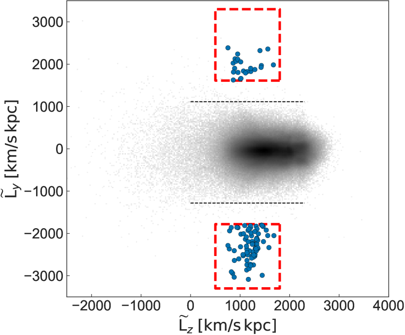
Figure 3: Distribution of stars from the 5D subset of Gaia, located within 15 degrees from the Galactic centre or anti-centre, in (pseudo)angular momentum space. The angular momenta are calculated here by assuming that the line-of-sight velocities are zero. The grey density map reveals the location of the stars, most of which are in the disk. The black dashed lines show the 2.5% and 97.5% quantiles of the $\widetilde{L}_{y}$-distribution. The two boxes indicated with red dashed lines are used to identify candidate members of the Helmi streams, here shown with blue symbols.

4 Analysis of the streams

4.1 Spatial distribution

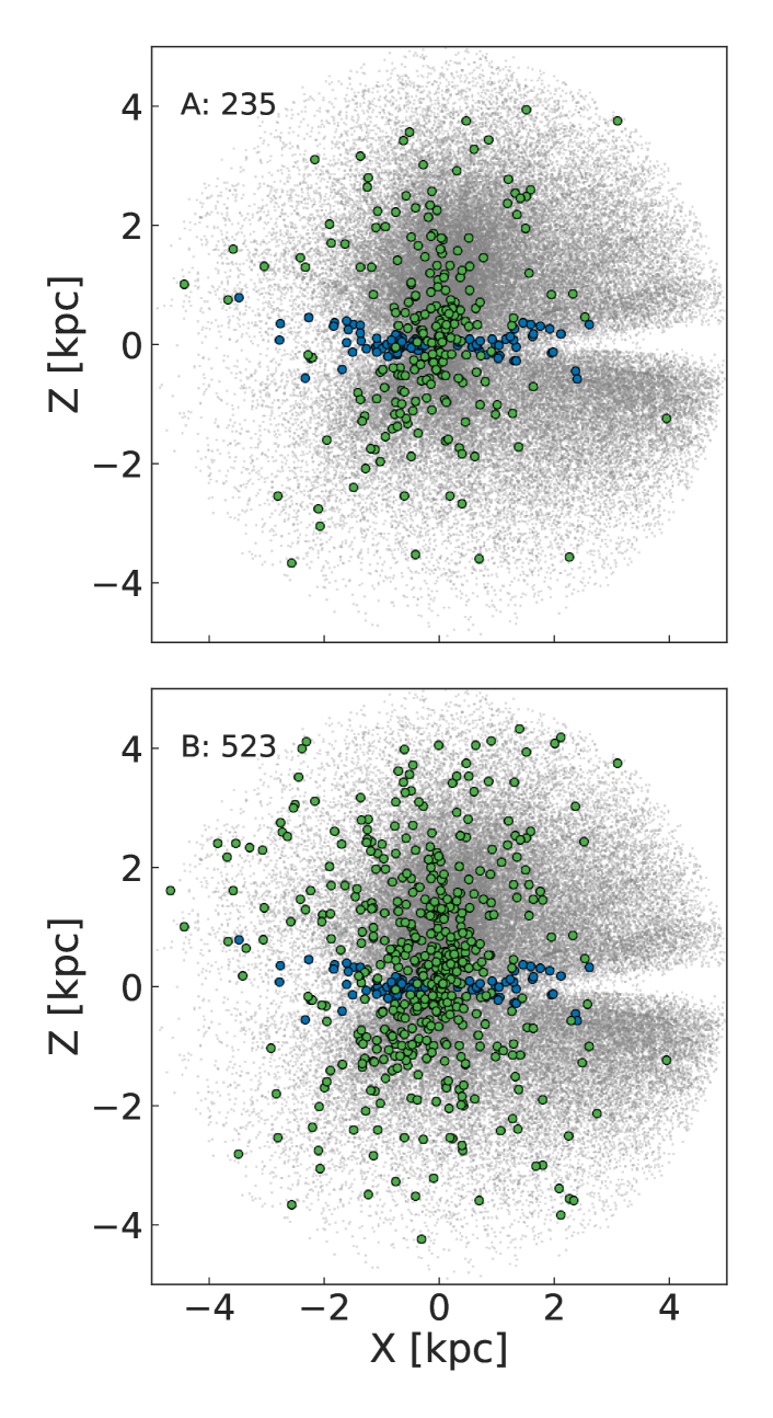
Figure 4: Distribution of members of the Helmi streams for the two selection boxes A (top) and B (bottom). The 6D stream members are indicated with green circles, local halo stars are shown in the background with grey symbols. The total number of 6D stream members is indicated in the top left of each panel. Tentative members from the 5D data set are shown with blue symbols.

Fig. 4 shows the distribution of the streams members in the $XZ$-plane, for the selection box A (top) and for B (bottom). Those identified with 6D information are indicated with green circles, a local sample of halo stars is shown in grey in the background. There is a lack of stars close to the plane of the disk, likely due to extinction (Gaia Collaboration, Katz et al., 2018). This gap is filled with tentative members from the 5D sample (in blue) which have, by construction, low galactic latitude. Fig. 4 reveals the streams stars to be extended along the $Z$-axis, as perhaps expected from their high $V_{Z}$ velocities, but there is also a clear decrease in the number of members with distance from the Sun.

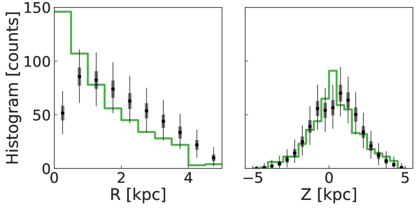
Figure 5: Distribution of heliocentric distance in the plane of the disk (left) and height above the plane (right) for stars in our 6D sample. The green histograms are for members of the Helmi streams. With black symbols, we show the mean counts obtained using $10^{4}$ random sets extracted from our (background) halo sample, with the grey and black error bars indicating the 1$\sigma$ and 3$\sigma$ uncertainties for each $R/Z$-bin. The Helmi streams are clearly more confined in the $R$-direction.

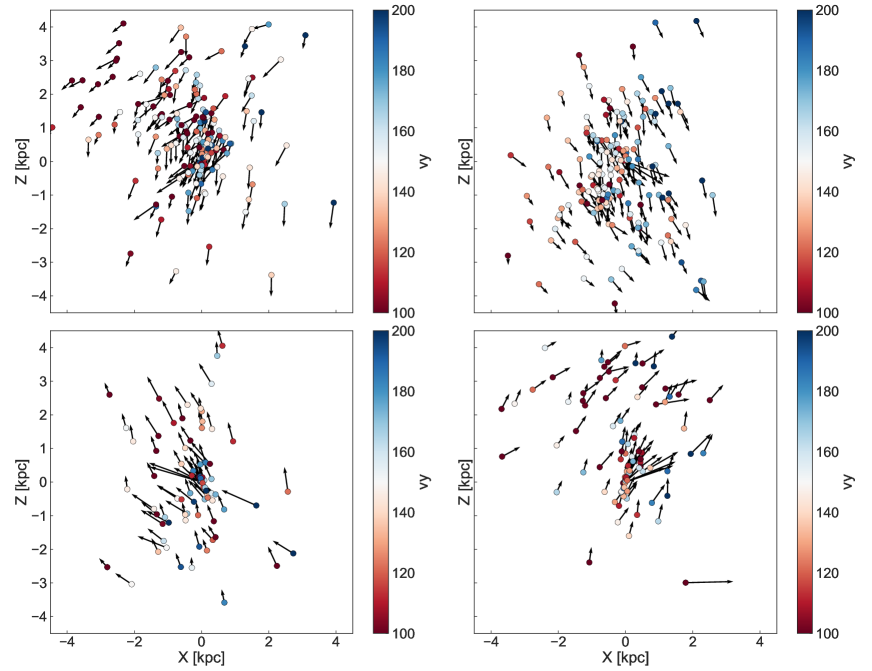
Figure 6: Distribution of the stars in the Helmi streams in the $XZ$ plane (i.e. perpendicular to the disk of the Milky Way), with the arrows illustrating their motions (amplitude and direction) in this plane. The symbols are colour-coded according to the amplitude of their $V_{Y}$ velocity (i.e. perpendicular to the projected plane). The top and bottom rows show stream members with $V_{Z}<0$ and $V_{Z}>0$, respectively. The left and right columns show stars with $V_{X}<0$ and $V_{X}>0$, respectively. In all the four panels streaming motions and substructures are clearly apparent.

To establish whether the spatial distribution of the streams differs from that of the background, we proceed as follows. We compare our sample of streams stars to $10^{4}$ samples randomly drawn from the background. The random samples contain the same number of stars as the streams, and the background comprises all of the stars in the halo sample, described in Section 2, excluding the streams members. In this way, we account for selection effects associated with the different footprints of the APOGEE/RAVE/LAMOST surveys as well as with the 20% relative parallax error cut (since the astrometric quality of the Gaia data is not uniform across the sky), and which are likely the same for the streams and the background.

Figure 5 shows a comparison of the distribution of heliocentric $R$ (left) and $Z$ (right) coordinates of the stars in our sample (in green) and in the random samples (black). The sizes of the grey and black markers indicate the 1$\sigma$ and 3$\sigma$ levels respectively, of the random samples. The $Z$-distribution of the streams members shows minimal differences with respect to the background, except near the plane, i.e. for $Z\sim 0$. On the other hand, their distribution in $R$ shows very significant differences with respect to the background, depicting a very steeply declining distribution. This was already hinted at in Fig. 6, and would suggest that the streams near the Sun have a cross section of $\sim 500$ pc.

4.2 Flows: velocity and spatial structure

The main characteristic of stars in streams is that they move together through space as in a flow. Figure 6 illustrates this by showing the spatial distribution of the members (according to selection B), in the $XZ\mbox{-}$plane. The arrows indicate the direction and amplitude of the velocities of the stars, with stars with $V_{Z}<0$ shown in the top row and those with $V_{Z}>0$ in the bottom row of the figure. Every star is colour-coded according to its velocity component in and out of the plane of projection (i.e. its $V_{Y}$). The left column shows stars with $V_{X}<0$, while the right column shows stars with $V_{X}>0$.

The flows seen in Fig. 6 reveal that the two characteristic clumps in $V_{Z}$ (i.e. those shown in the left panel of Fig. 1) actually consist of several smaller streams. For example, the top and bottom right panels of Fig. 6 both clearly show two flows: one with $V_{X}\sim 0$, the other with a large $V_{X}$.

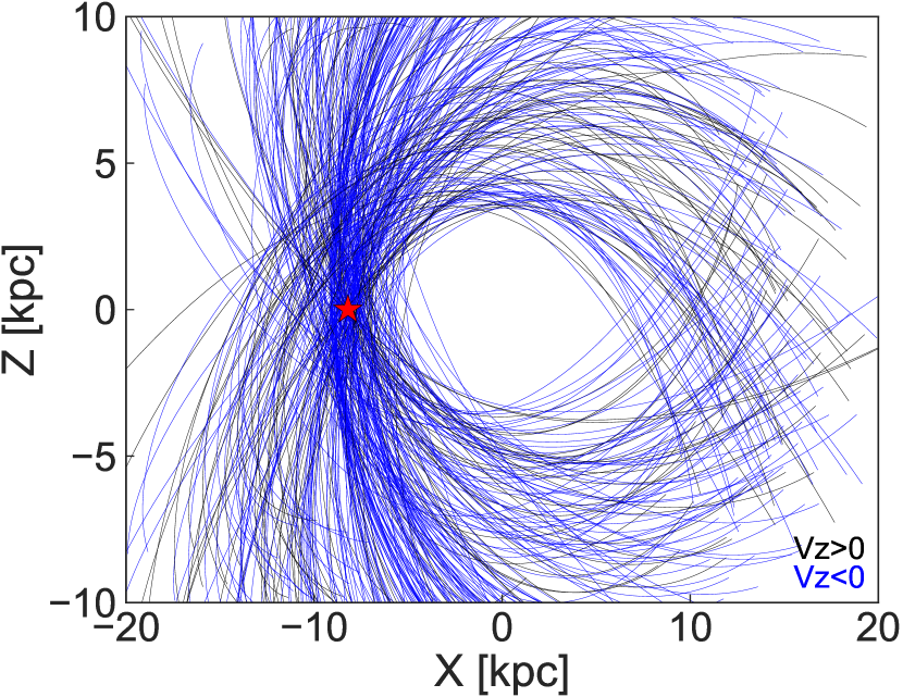
Figure 7: Compilation of orbits based on the 6D positions of the members of the Helmi streams. These orbits have been integrated for 100 Myr backwards and forward in time. The position of the Sun is illustrated with a red star, the Galactic centre is at $(X,Z)=(0,0)$ in this frame. The trajectories of stars that currently have $V_{Z}>0$ are coloured black, while those with $V_{Z}<0$ are shown in blue. Close to the Solar position, the majority of the Helmi streams’ members move perpendicular to the plane of the disk, and are close to pericentre.

To enhance the visibility of the flows we integrate the orbits of the streams stars forward and backwards in time. The potential in which the orbits are calculated is the same as the one described in Section 3.2. The trajectories of all the stars are integrated for $\pm 100$ Myr in time and are shown in Fig. 7 projected onto the $XZ$ plane. With a red star, we indicate the Solar position. The trajectories of stars that belong to the group with $V_{Z}>0$ are coloured black, while those with $V_{Z}<0$ are given in blue.

Clearly, the stars found in the Solar vicinity are close to an orbital turning point and on trajectories elongated in the $Z$-direction, as expected from their large vertical velocities. Fig. 7 serves also to understand the observed spatial distribution of the member stars (i.e. narrower in $X$ (or $R$) and elongated in $Z$) seen in Fig. 4. Finally, we also note the presence of groups of orbits tracing the different flows just discussed, such as for example the group of stars moving towards the upper left corner of the figure (and which corresponds to some of the stars shown in the bottom left panel of Fig. 6).

4.3 Ratio of the number of stars in the two $V_{Z}$ streams

As mentioned in the introduction, the ratio of the number of stars in the two $V_{Z}$ streams was used in Kepley et al. (2007) to estimate the time of accretion of the object. The ratio these authors used was 1:2, in good agreement with the ratio found here in §3.1 for the core members. Using numerical simulations, this implied an accretion time of $6-9$ Gyr for an object of total dynamical mass of $\sim 4\times 10^{8}$ M_⊙. Now with a sample of up to 523 members, we will analyze how this ratio varies when exploring beyond the immediate Solar vicinity.

Figure 8 shows the ratio of the number of stars in the two streams in $V_{Z}$ for selection B, as a function of the extent of the volume considered. Blue indicates the ratio of all the stars and green is for the 6D Gaia-only sample. The central lines plot the measured ratio and the shaded areas correspond to the 1$\sigma$ Poissonian error, showing that there is good agreement between the samples. The dashed lines at 1:2, 3:5 and 2:5 encompass roughly the mean and the scatter in the ratio. Evidently, the ratio drops slightly beyond the $1$ kpc volume around the Sun, however, overall it stays rather constant and takes a value of approximately 1:2 for stars with $V_{Z}>0$ relative to those with $V_{Z}<0$.

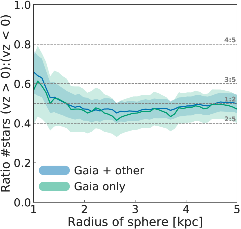
Figure 8: Ratio of the number of stars in the two clumps in $V_{Z}$ using selection box B, for different volumes and for the two samples of stars as indicated. The shaded area corresponds to the Poisson error on the measured ratio.

4.4 HR diagram and metallicity information

Photometry from Gaia combined with auxiliary metallicity information from the APOGEE/RAVE/LAMOST surveys can give us insights into the stellar populations of the Helmi streams. By using the Gaia parallaxes we construct the Hertzsprung-Russell (HR) diagram shown in Fig. 9. We have used here a high photometric quality sample by applying the selection criteria from Arenou et al. (2018) and described in Section 3.3. Note that since the photometry in the BP passband is subject to some systematic effects especially for stars in crowded regions (see Gaia Collaboration, Brown et al., 2018), we use ($G-G_{\mathrm{RP}}$) colour.

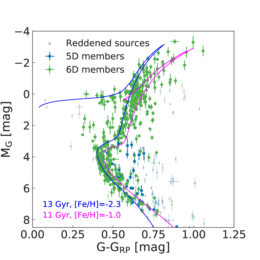
Figure 9: Hertzsprung-Russel diagram of members of the Helmi streams. Those identified in the 6D sample are shown in green, while those without radial velocities are indicated with blue symbols. Members that are likely highly reddened are indicated in light grey. Superimposed are single population isochrones taken from Marigo et al. (2017). They serve to illustrate that the Helmi streams include a range of old, metal-poor stellar populations which did not form in a single event.

In Fig. 9 the stream members from the 6D sample are plotted with green symbols, and in blue if they are from the 5D dataset. On the basis of a colour-colour diagram we have identified stars that are likely reddened by extinction, and these are indicated with light grey dots. Since most stars follow a well-defined sequence in the $[(G-G_{\mathrm{RP}}),(G-G_{\mathrm{BP}})]$ space, outliers can be picked out easily. We consider as outliers those stars with a $(G-G_{\mathrm{BP}})$ offset greater than $0.017$ from the sequence (i.e. 5$\times$ the mean error in the colours used). We find that especially the members found in the 5D dataset appear to be reddened. This is expected as all of these stars are located at low Galactic latitude (within 15 degrees from the galactic centre or anti-centre). Fig. 9 shows also that we are biased towards finding relatively more intrinsically bright than fainter stars, and this is due to the quality cuts applied and to the magnitude limits of the samples used. We expect however that there should be many more fainter, lower main sequence stars that also belong to the Helmi streams, hidden in the local stellar halo.

The HR diagram shown in Fig. 9 does not resemble that of a single stellar population, but rather favours a wide stellar age distribution of $\sim 2$ Gyr spread, based on the width of the main sequence turn-off. To illustrate this we have overlayed two isochrones from Marigo et al. (2017) for single stellar populations of 11 and 13 Gyr old age and with metallicities [Fe/H] $=-1.0$ and $-2.3$ respectively. Note that to take into account the difference between the theoretical and actual Gaia passbands (Weiler, 2018), we have recalibrated the isochrones on globular clusters with similar age and metallicity (NGC104, NGC6121, NGC7099, see Harris, 1996), which led to a shift in ($G-G_{\mathrm{RP}}$) colour of 0.04 mag.

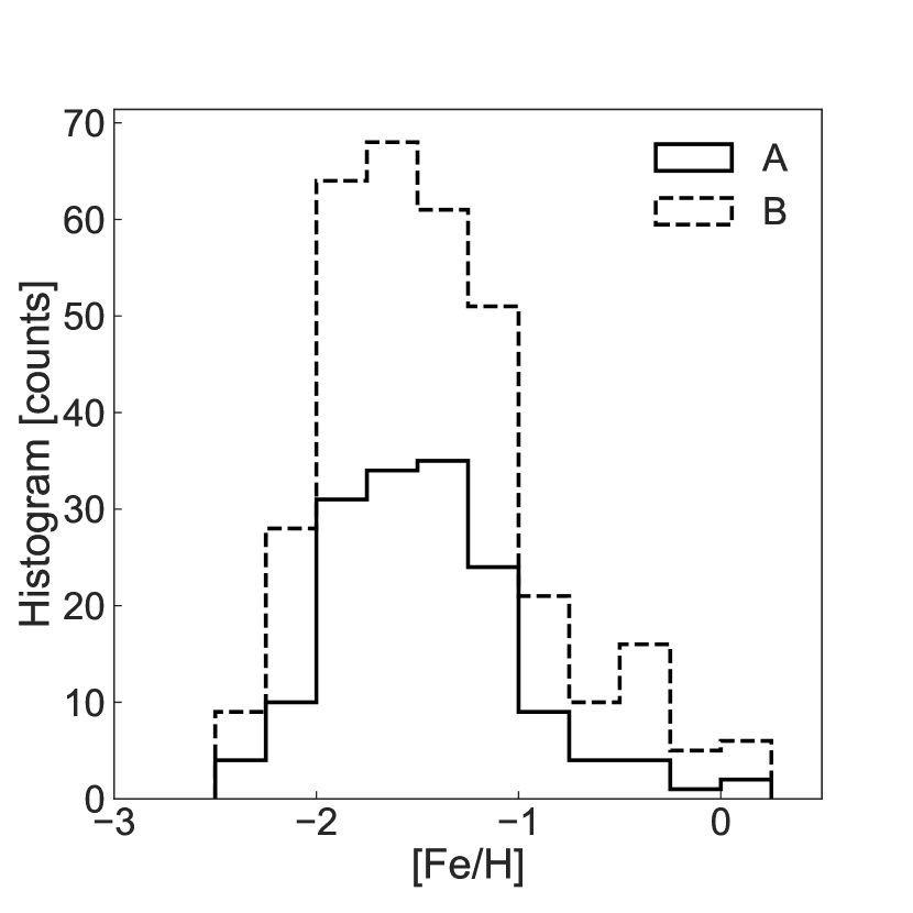
Figure 10: Histogram of the metallicities of the Helmi streams stars that are in the APOGEE/RAVE/LAMOST datasets. The distributions are very similar for selections A & B, peaking at [Fe/H] $\sim-1.5$ and revealing a broad range of metallicities for the Helmi streams stars. The metal-rich tail ([Fe/H] $\sim$ $-0.5$) is likely due to contamination from the thick disk but it is minimal for both selection boxes.

The spread in metallicities used for the isochrones is motivated by the metallicity distribution shown in Figure 10, and derived using the stream members found in the APOGEE/RAVE/LAMOST datasets. We have used the following metallicity estimates for the different surveys: Met_K for RAVE, FE_H for APOGEE and feh for LAMOST. The distribution plotted in Fig. 10 shows a range of metallicities [Fe/H] $=[-2.3,-1.0]$, with a peak at [Fe/H] $=-1.5$. The small tail seen towards the metal-rich end, i.e. at [Fe/H] $\sim-0.5$ is likely caused by contamination from the thick disk. The shape of the distribution shown in Figure 10 is reminiscent of that reported by Klement et al. (2009) and by Smith et al. (2009) for much smaller samples of members of the Helmi streams. Roederer et al. (2010) have carried out detailed abundance analysis of the original stream members which confirm the range of $\sim 1\,\mathrm{dex}$ in [Fe/H] found here. All this evidence corroborates that the streams originate in an object that had an extended star formation history.

5 Simulating the streams

We focus here on N-body experiments we have carried out to reproduce some of the properties of the Helmi streams. To this end, we used a modified version of GADGET 2 (Springel et al., 2005) that includes the host rigid, static potential described in section Section 3.2 to model the Milky Way.

The analysis presented in previous sections, and in particular the HR diagram and metallicity distribution of member stars, supports the hypothesis that the Helmi streams stem from a disrupted (dwarf) galaxy. We therefore model the progenitor of the streams as a dwarf galaxy with a stellar and a dark matter component. We consider four possible progenitors whose characteristics are listed in Table 2.

For the stellar component, we use $10^{5}$ particles distributed following a Hernquist profile, whose structural properties are motivated by the scaling relations observed for dwarf spheroidal galaxies (Tolstoy et al., 2009). For the dark matter halo we use $6\times 10^{5}$ particles following a truncated NFW profile (similar the model introduced in Springel & White, 1999, but where the truncation radius $\text{r}_{\textrm{c,trunc}}$ and the decay radius $\text{r}_{\textrm{d,trunc}}$ are specified independently), with characteristic parameters taken from Correa et al. (2015). We truncate the NFW halo at a radius where its average density is three times that of the host (at the orbital pericentre). After setting the system up using the methods described in Hernquist (1993), we let it relax for 5 Gyr in isolation. We then place it on an orbit around the Milky Way. This orbit is defined by the mean position and velocity of the stars that were identified as core members of the stream with $V_{Z}<0$.

Table 2: Structural parameters of the simulated dwarf galaxies. Note that we quote both the dark halo’s original and truncated mass. This truncation depends on two parameters: $\text{r}_{\textrm{c,trunc}}$ and $\text{r}_{\textrm{d,trunc}}$, the cut-off and the decay radii, respectively.

	prog. 1	prog. 2	prog. 3	prog. 4
$\text{M}_{*}$ ($\text{M}_{\odot}$)	$5\cdot 10^{6}$	$10^{7}$	$5\cdot 10^{7}$	$10^{8}$
$\text{r}_{s,*}$ (kpc)	0.164	0.207	0.414	0.585
$\text{r}_{\text{s,NFW}}$ (kpc)	1.32	1.72	3.42	4.26
$\text{M}_{\textrm{dm}}$ ($\text{M}_{\odot}$)	$5\cdot 10^{8}$	$10^{9}$	$5\cdot 10^{9}$	$10^{10}$
$\text{M}_{\textrm{dm,trunc}}$ ($\text{M}_{\odot}$)	$1.9\cdot 10^{8}$	$3.8\cdot 10^{8}$	$1.84\cdot 10^{9}$	$3.62\cdot 10^{9}$
$\text{r}_{\textrm{c,trunc}}$ (kpc)	2.0	2.5	4.1	5
$\text{r}_{\textrm{d,trunc}}$ (kpc)	0.65	0.86	1.62	2.13

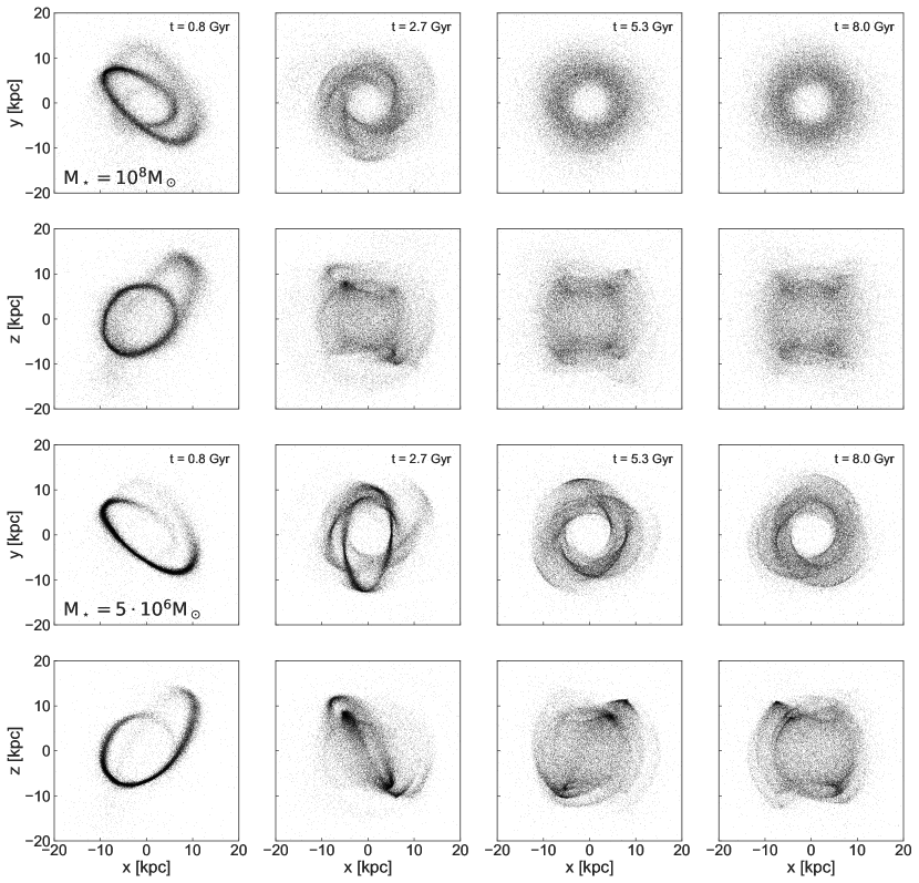
Figure 11: Spatial evolution of the Helmi streams at four different snapshots in our simulations. The top two rows show the evolution of a progenitor with a stellar mass of $10^{8}\mathrm{M}_{\odot}$, while the bottom two rows correspond to a system with a stellar mass of $5\times 10^{6}\mathrm{M}_{\odot}$. In both cases, the orbit of the progenitor is the same. The appearance of the debris is seen to depend on the time since accretion as well as on the mass of the progenitor.

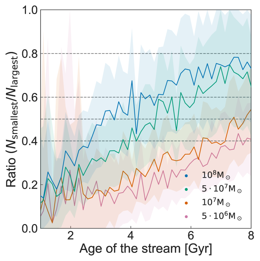
Figure 12: Ratio of the numbers of stars in the less populated $V_{Z}$ clump compared to that of the more populated clump, as a function of time for our N-body simulations. The solid lines show the mean values, averaged over 25 different volumes spread uniformly along a circle of 1 kpc at the Solar radius.

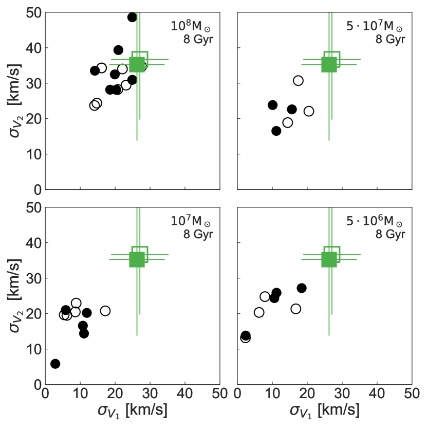
Figure 13: Velocity dispersions of the simulated streams 8 Gyr after accretion. These have been computed using the principal axis of the velocity ellipsoid of stars in a given $V_{Z}$ clump, open/closed markers are used for the smallest/largest clump respectively. We show the results for volumes satisfying the ratio in the number of stars in the clumps as observed for the data. The green markers indicate the measured velocity dispersion from the data, the error bars illustrate the scatter in 1000 randomly downsampled sets of the streams members.

Figure 11 illustrates the evolution of a high mass dwarf galaxy in the top two rows, and for a low mass dwarf galaxy in the bottom two rows. In each panel, we show the star particles in galactocentric Cartesian coordinates for different times up to 8 Gyr after infall. This comparison shows that increasing the mass results in more diffuse debris. On the other hand, the time since accretion has an impact on the length of the streams and on how many times the debris wraps around the Milky Way.

5.1 Estimation of the mass and time of accretion

To constrain the history of the progenitor of the Helmi streams we use the ratio of the number of stars in the two clumps in $V_{Z}$ as well as their velocity dispersion. Typically, the simulated streams do not have a uniform spatial distribution and they also show variations on small scales. Furthermore, the azimuthal location of the Sun in the simulations is arbitrary. Therefore, and also to even out some of the small-scale variations, we measure the ratio of the number of stars in the streams and their velocity dispersion in 25 volumes of 1 kpc radius located at 8.2 kpc distance from the centre, and distributed uniformly in the azimuthal angle $\phi$.

Fig. 12 shows the mean of the ratio for the different volumes as a function of time with solid curves, with the colours marking the different progenitors listed in Table 2. The shaded areas correspond to the mean Poissonian error in the measured ratio for the different volumes. The horizontal dashed lines are included for guidance and correspond to the lines shown in Fig. 8 for the actual data.

The mean ratio is clearly correlated with the properties of the progenitor, the most massive one being first to produce multiple streams in a given volume. Massive satellites have a larger size and velocity dispersion, which causes them to phase mix more quickly because of the large range of orbital properties (energies, frequencies). Based solely on Fig. 12, and taking a ratio between 0.55 and 0.7 as found using the Gaia-only sample in a 1 kpc sphere, we would claim that there is a range of possible ages of the stream, with the youngest being $\sim 4.5$ Gyr for the most massive progenitor, while for the lowest mass object the age would have to be at least 8 Gyr.

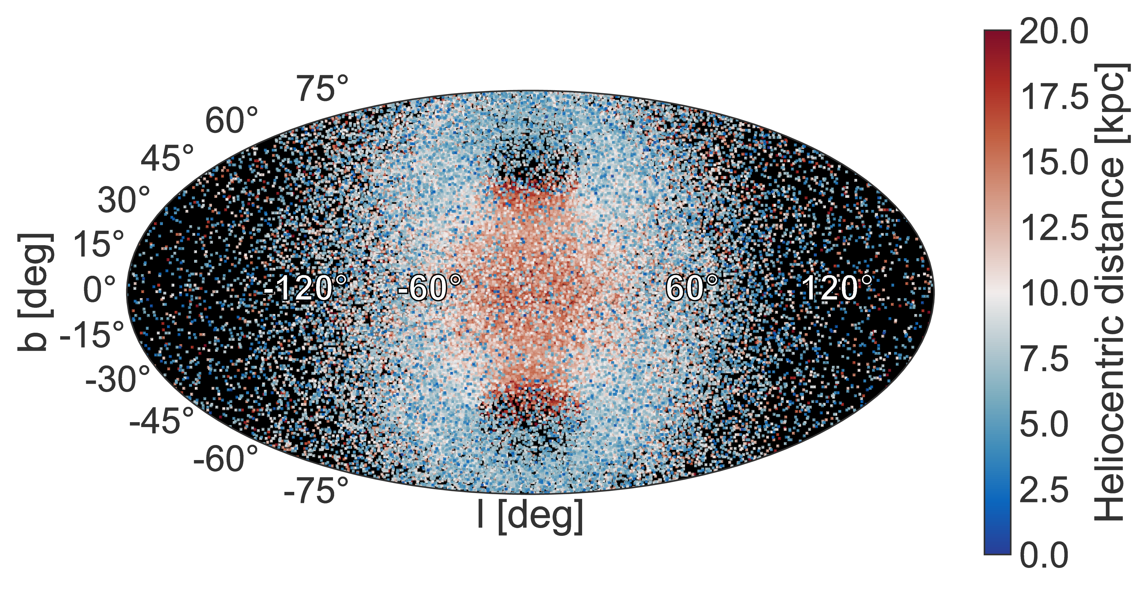
Figure 14: Mollweide projection in Galactic sky coordinates $l$ and $b$ of the distribution of star particles for the simulation of a progenitor dwarf galaxy with a stellar mass of $10^{8}\,\mathrm{M}_{\odot}$. The colour-coding gives the heliocentric distance of the particles.

A different way of probing the properties of the progenitor is to use the velocity dispersion of the streams. In Fig. 13 we show the dispersion along two principal axes of the velocity ellipsoid for the 1 kpc volumes that satisfy the ratio-constraint on the number of stars in the two $V_{Z}$ clumps, with open/closed markers used for the least/most populated clump. Green markers indicate the measured velocity dispersions. Typically the simulations have fewer particles in such 1 kpc volumes than observed in the debris. Therefore, we down-sample the data to only 15 stars per stream, which corresponds to the average number of particles in the simulations. The error bars indicate the maximum scatter in the velocity dispersion for 1000 such random downsampled sets.

The ellipsoid is roughly aligned in cylindrical coordinates with $V_{1}$, $V_{2}$, and $V_{3}$ corresponding respectively to $V_{\phi},\,V_{Z},\,V_{R}$. Note that only for the most massive progenitor (and for times ¿ 5 Gyr) the velocity dispersions are in good agreement with the observed values for $\sigma_{V1}$ and $\sigma_{V2}$, and that in all the remaining simulations, the dispersions are too small compared to the data. We should point out however, that the largest velocity dispersion (i.e. that along $V_{R}$) is less well reproduced in our simulations, possibly indicating that the range of energies of the debris is larger. However, if we clip 1$\sigma$ outliers in $V_{R}$ for the data, and recompute $\sigma_{V3}$, we find much better agreement with the simulations (while the values of $\sigma_{V1}$ and $\sigma_{V2}$ remain largely the same). The clipped members of the Helmi streams are all in the high energy, $E$, tail (see Fig.2), suggesting perhaps that the object has suffered some amount of dynamical friction in its evolution.

Combining the information of the ratio (Fig. 12) and the corresponding velocity dispersion measurements ( Fig. 13) we therefore conclude that the most likely progenitor of the Helmi streams was a massive dwarf galaxy with a stellar mass of $\sim 10^{8}\,\mathrm{M}_{\odot}$. In general, the simulations suggest a range of plausible accretion times from $5-8$ Gyr. Although these estimates of the time of accretion are different than those obtained by Kepley et al. (2007), our results are consistent when a similar progenitor mass is used (i.e. of models 1/2), which however, does not reproduce well the observed kinematical properties of the streams.

5.2 Finding new members across the Milky Way

To investigate where to find new members of the Helmi streams beyond the Solar neighbourhood we turn to the simulations.

In Fig. 14 we show a sky density map of stars from the N-body simulation corresponding to the dwarf galaxy with $M_{*}=10^{8}\,\mathrm{M}_{\odot}$, 8.0 Gyr after accretion. The coordinates shown here are galactic $l$ and $b$ plotted in a Mollweide projection with the Galactic centre located in the middle (at $l=0$). Note that nearby stars (in blue) are mainly distributed along a “polar ring-like” structure between longitudes $\pm 60^{\circ}$ (see for comparison Fig. 6). The most distant members are found behind the bulge (in red), but because of their location they may be difficult to observe.

6 Association with globular clusters

If the progenitor of the Helmi streams was truly a large dwarf galaxy, it likely had its own population of globular clusters (see Leaman et al., 2013; Kruijssen et al., 2018). To this end we look at the distribution of the debris in IOM-space for the simulation of the progenitor with $M_{*}=10^{8}\,\mathrm{M}_{\odot}$ and overlay the data for the globular clusters from Gaia Collaboration, Helmi et al. (2018).

Figure 15 shows the energy $E$ vs $L_{z}$ (top) and the $L_{\perp}$ vs $L_{z}$ (bottom) of star particles in the simulation (black) and the stream members (green) together with the globular clusters (white open circles). We have labelled here the globular clusters that show overlap with the streams members in this space. Those that could tentatively be associated on the basis of their orbital properties are: NGC 4590, NGC 5024, NGC 5053, NGC 5272, NGC 5634, NGC 5904, and NGC 6981.

This set of globular clusters shows a moderate range in age and metallicity: they are all old with ages $\sim 11-12$ Gyr and metal-poor with metallicities [Fe/H] = [$-2.3$,$-1.5$]. These age estimates are from Vandenberg et al. (2013), while for NGC 5634 we set it to $12$ Gyr from comparison to NGC 4590 based on the zero-age HB magnitude (Bellazzini et al., 2002), and assume an uncertainty of 0.5 Gyr. Interestingly, Fig. 16 shows that the clusters follow a relatively tight age-metallicity relation, and which is similar to that expected if they originate in a progenitor galaxy of $M_{*}\sim 10^{7}-10^{8}\,\mathrm{M}_{\odot}$ (see Leaman et al., 2013, Fig. 4).

Fig. 17 shows the Gaia colour-magnitude diagrams (CMD) of the globular clusters tentatively associated with the Helmi streams. Although not all CMDs are well-populated because of limitations of the Gaia DR2 data, their properties do seem to be quite similar, increasing even further the likelihood of their association to the progenitor of the Helmi streams.

Some of the associated globular clusters, namely NGC 5272, NGC 5904, and NGC 6981 have in fact, been suggested to have an accretion origin (of a yet unknown progenitor, see Kruijssen et al., 2018, and references therein). Two other clusters, NGC 5024 and NGC 5053, have at some point been linked to Sagittarius, although recent proper motion measurements have demonstrated this association is unlikely (see Law & Majewski, 2010; Sohn et al., 2018; Gaia Collaboration, Helmi et al., 2018). Also NGC 5634 has been related to Sagittarius (Law & Majewski, 2010; Carretta et al., 2017) based on its position and radial velocity. However, the proper motion of the system measured by Gaia Collaboration, Helmi et al. (2018) is very different from the prediction by for example, the Law & Majewski (2010) model of the Sagittarius streams.

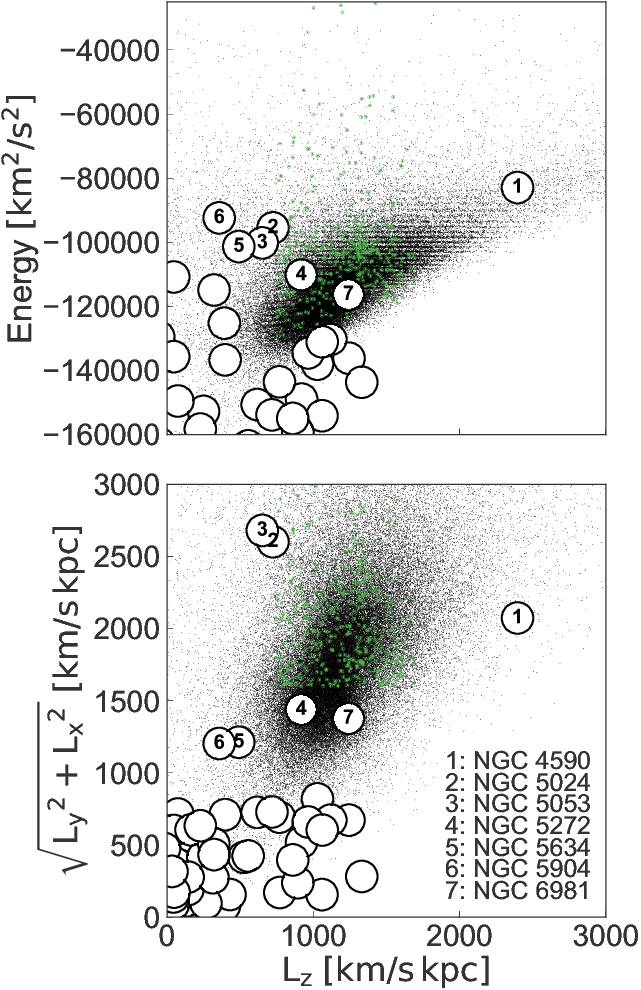
Figure 15: $E-L_{z}$ (top) and the $L_{\perp}-L_{z}$ (bottom) distributions of the simulated stars (in black), together with the selected 6D stream members (in green). Plotted here are the star particles from the simulation of the most massive dwarf, with a stellar mass of $10^{8}\,\mathrm{M}_{\odot}$ and accretion time of 8.0 Gyr. Large symbols indicate the location of Milky Way globular clusters. Those possibly associated with the Helmi streams based on their location in these panels are numbered.

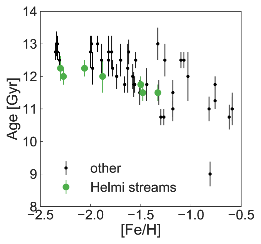
Figure 16: Age-metallicity distribution of Milky Way globular clusters based on Vandenberg et al. (2013). The green symbols mark the clusters associated with the Helmi streams on the basis of their orbital properties. They follow a well-defined age-metallicity relation.

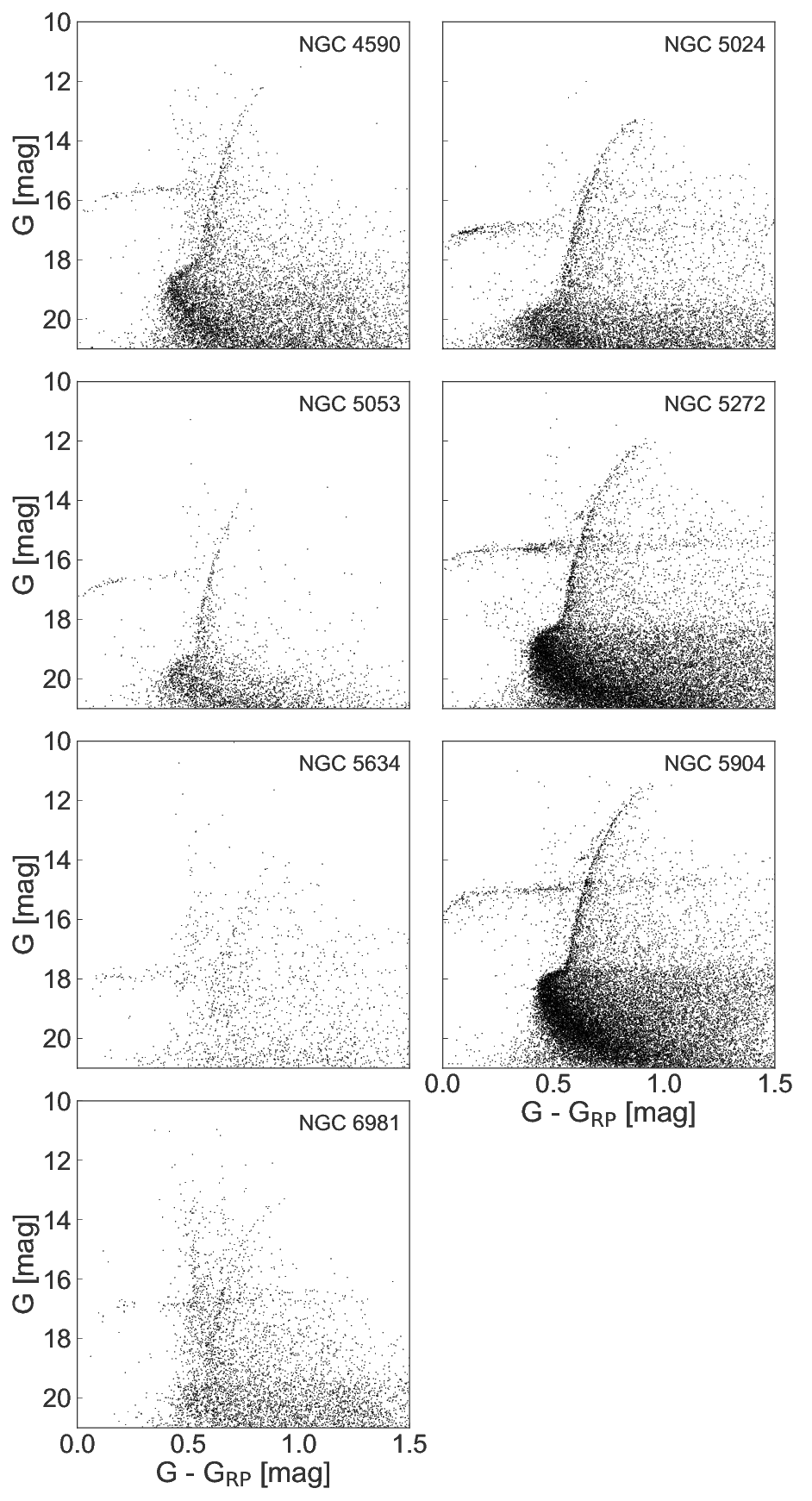
Figure 17: Gaia colour-magnitude diagrams for the globular clusters that are likely associated with the Helmi streams on the basis of their orbital properties. All the CMDs correspond to stellar populations that are old and metal-poor.

7 Conclusions

Using the latest data from Gaia DR2 combined with the APOGEE/RAVE/LAMOST surveys we find hundreds of new tentative members of the Helmi streams. In the 6D sample that we built, we identified 523 members on the basis of their orbital properties, in particular their energy and angular momenta. On the other hand, we found 105 stars in the full Gaia 5D dataset in two 15^o-radius fields around the galactic centre and anticentre, using only the tangential velocities of the stars (which translate directly into two components of their angular momenta). Despite the large number of newly identified members we expect that many, especially faint stars are still hiding, even within a volume of 1 kpc around the Sun.

Having such an unprecedented sample of members of the streams allows us to characterize the streams and the nature of their progenitor. The HR diagram of the members suggests an age range of $\sim 11-13$ Gyr, while their metallicity distribution goes from [Fe/H] $\sim-2.3$ to $-1.0$, with a peak at [Fe/H]$\sim-1.5$. We are also able to associate to the streams seven globular clusters on the basis of their dynamical properties. These clusters have similar ages and metallicities as the stars in the streams. Remarkably they follow a well-defined age-metallicity relationship, and similar to that expected for clusters originating in a progenitor galaxy of $M_{*}\sim 10^{7}-10^{8}\,\mathrm{M}_{\odot}$ (Leaman et al., 2013).

This relatively high value of the stellar mass is also what results from N-body simulations that aim to recreate the observed dynamical properties of the streams. From the ratio of the number of stars in the two clumps in $V_{Z}$ and their velocity dispersion we estimate the time of accretion to be in the range $5-8$ Gyr and a stellar mass for the dwarf galaxy of $\sim 10^{8}\mathrm{M}_{\odot}$.

Although 5 Gyr ago would imply a relatively recent accretion event, one might argue that the object was probably on a less bound orbit and sunk in via dynamical friction (thanks to its large mass) and started to get disrupted then. This could explain the mismatch between the age of the youngest stars in the streams (approximately 11 Gyr old), and the time derived dynamically.

Despite the fact that the simulations are able to recreate the observations reasonably well, they fail to reproduce fully the observed velocity distribution in particular in the radial direction. This could be due to the lack of dynamical friction, but also by the limited exploration of models for the potential of the Milky Way. Other important improvements will be to consider the inclusion of gas particles and star formation in the simulations, as well as different initial morphologies for the progenitor systems (not only spherical, but also disk-like).

Originally, H99 determined that 10% of the stellar halo mass beyond the Solar radius could belong to the progenitor of the Helmi streams. The lack of a significant increase in the number of members subsequently discovered by other groups (Chiba & Beers, 2000), led to the suggestion that the fraction may be lower. Our best estimate of the stellar mass of the progenitor of the Helmi stream is $\sim 10^{8}\,\mathrm{M}_{\odot}$, implying that it does significantly contribute to the stellar halo. For example Bell et al. (2008) estimate a stellar mass for the halo of $(3.7\pm 1.2)\times 10^{8}\,\mathrm{M}_{\odot}$ between galactocentric radii of 1 to 40 kpc, and hence being a lower limit to the total stellar halo mass. Other estimates, based on the local density of halo stars give $7-10\times 10^{8}\mathrm{M}_{\odot}$ (see Morrison, 1993; Bland-Hawthorn & Gerhard, 2016). This implies that the Helmi streams may have contributed $\sim 10-14\%$ of the stars in the Galactic halo.

Appendix: Table of members selection B

Table A3: Gaia DR2 source_ids for selection B

IDs members 1-105	IDs members 106-210	IDs members 211-315	IDs members 316-419	IDs members 420-523
4641558272441088	15542185269834624	18721418846252288	25052342374772736	40341188999965056
44825306655035520	47948469433052800	48191667661477120	66174455213158656	88903903177506304
109717108535569920	114370963299054720	129029789761784320	133659416611738496	148992625953529216
166864465909649024	208313266841386496	214416419665198976	277505056837614336	297601582475179520
298510126972435200	300034840362494592	317928636190603136	328660281995935232	334897296063939712
338420371837484160	362606329112459136	365903386527108864	371779211025724032	378336075603390208
414268497862196224	424315422799326464	565085174940343296	571826104634521856	579282859350500480
579472799984173824	580075916471255040	597915355193425152	601485847406210688	604095572614068352
609634774756212480	613717261429518336	618362698056754816	623835615967986560	640225833940128256
641011469357926144	641984640227836288	642298482077861888	650878108749480960	658200993629082240
660857241923470336	666167814367063296	675824721913920768	676184743253306752	690133560079137920
694677944716195712	695472307507752320	703875080308465536	711475458731171712	715176071273608704
720354564881582080	721179847141106816	722255002009942528	722917384750970752	724057994920894592
724067027236448128	731949048138844800	735896535401139072	777558680244658176	780787744032780544
793157490364148224	795010747276301952	809190053525078272	809488433492803072	809944799537192320
812131247128723712	814140020513681024	821455518049745280	838151499037299328	839367249661110912
839618793008582272	840616123070439552	841170654888167808	842363247047642368	845266198261944960
846326471068781824	849565494885493888	850419781060360448	868447614227967744	877174369298101504
877928256318192512	878629435499205632	879194790634452352	879287699366827520	885358240501948032
892436552763913344	894379527249498496	900194908672475648	901431176354580480	909255575975553920
924073900341372160	926019211289351424	941117327005728000	951217299082189696	961149020114863872
975473938637155968	1011601034570885504	1021904837208334848	1022757474116502400	1022993078842418432
1033400437435614976	1049376272667191552	1143069060084735232	1155172720304980224	1160604689999075456
1176187720407158912	1179353424836990720	1190457117888556160	1211628386079715840	1243915819907387392
1244298759191228800	1255012675370113536	1258514207587827840	1260211058971256320	1261193202028905600
1262839514533098368	1263921674493183488	1264302346034442496	1275876252107941888	1278333454435460096
1278999758481584768	1286475922158536064	1288312793771274880	1317046296776785920	1319060876956649216
1325856580370512768	1329198236725539456	1351435584519064576	1358807878703209472	1359836093873456768
1361390494077900672	1375199947805963520	1375468537880511488	1376687518318241536	1390150935120171776
1403917336097206144	1415635209471360256	1416077522383596160	1426065314211359488	1445550069004682368
1454211574931259008	1454848260885706240	1459258161504411776	1461351734723634944	1465018949599024000
1467009581041527168	1469066526780349312	1471944223587079808	1472043763749113984	1475499116478182400
1476416280975128832	1479656885339494656	1481262412833531520	1484142927140574976	1485907299704041088
1498477363310839168	1500489435229902976	1501129694594779776	1501277853786344704	1512783143459215744
1516361572771506176	1516500901510616960	1522392875086096384	1527475951701753984	1529110474518977920
1532216221205478272	1533286423976243584	1534269318651955072	1543128667952320384	1543778891645673216
1544941144151976832	1550080089702483584	1559682880662202240	1561486148450638080	1576029045153304448
1590912446864098688	1595706764237530624	1601706279498493184	1601734905456540160	1603695231610033024
1606083435288423680	1609793702916552448	1616751038836648192	1618407796700425856	1621470761217916800
1639946061258413312	1651212997426399872	1659006954318690688	1661132860050868096	1680352357664352384
1687099201530228352	1688495581297486336	1740372429681699712	1741837288407560192	1746823363186399104
1770226575557939840	1785179585801889792	1880722993023978240	1897394608662403584	1909569058536197760
1915730687339037056	1920542906137425664	1927742920592283264	1959250663239949568	1969372801649974656
2075971480449027840	2081319509311902336	2090990366909021312	2107177716389487744	2113756098755468288
2118428129820961152	2119154219811372928	2143783830030463744	2152492992912794112	2223355928911050752
2268048503896398720	2290361477475441664	2322233192826733184	2344587054493724288	2355425387285206016
2373208853993082112	2416023871138662784	2417033428971348608	2436947439975372672	2438115774159097856
2447968154259005952	2463622347979629952	2484686482506940416	2492679893385490944	2493751577920673664
2497639347957300096	2515939172813427840	2518385517465704960	2519551171589880192	2533982360488142336
2548084666562636544	2549249942728874368	2556488440091507584	2562681954730905344	2564879259999378560
2565036284003715712	2565305629992853376	2568434290329701888	2577125551790493824	2577340815551111680
2577877377225342464	2585460292309803264	2587112141027257472	2593008821887179008	2593099428517326848
2597454555419529728	2604228169817599104	2610361657994140032	2652715636170048384	2658069914200047872
2670534149811033088	2681582248805460864	2685833132557398656	2702017668840521088	2710316816966218496
2715380235515703168	2716342071966879744	2731449911488518144	2747904614098575488	2753048786625056640

Table A4: Gaia DR2 source_ids for selection B - extended

IDs members 1-105	IDs members 106-210	IDs members 211-315	IDs members 316-419	IDs members 420-523
2753174783785251328	2762507266682585728	2763829601214919040	2777125789169639296	2777896134503915648
2782868607121209344	2807804328248244224	2816029465498234368	2838661293152878976	2841291982098062208
2865194471533729152	2865540508457717376	2866048379751327616	2869555134648788736	2876439211309388672
2882203332298969728	2890470899529272832	2891152566675457280	2901753198796969216	2902505745786910080
2954185571135157504	2959451922593403904	2964823797107665664	3074369755487517184	3085891537839264896
3085891537839267328	3124268582457078400	3140633331268375296	3165682645690499840	3179127443812906880
3191801342547132544	3202308378739431936	3214420461393486208	3233974932096638592	3236724913756362624
3244220864341745920	3246220914649655552	3258304272560352128	3267948604442696448	3270247545819617792
3275579971053642624	3283448591659397504	3302997083768142464	3306026508883214080	3311451812788556800
3318466112860232832	3344421699741253376	3360259919923274496	3368025671769397120	3368344461421835776
3375760083236221568	3435000842026369280	3458106907086594304	3500260464905928832	3515304597176877056
3520836313191203584	3612787302391075968	3638008690382625408	3638308577883569024	3642005964905520384
3645723619877700352	3649703023041037696	3665517234359034752	3667980999398592384	3685879227632832640
3693613948337587456	3694894948103300608	3696531536801618560	3697949460124343296	3697998658974002944
3698500933925098496	3700419135039744896	3703984129693916928	3705595086027166976	3710778767956154112
3712313170791794944	3712995761354141184	3716710186510880256	3718269255344140288	3719989475645411712
3726338021425401728	3734341989334114304	3736775002407500416	3738979076544369920	3742101345970116224
3742977210060826496	3767256797623849984	3773582902198012800	3784512979787195008	3786952418131994880
3798431869281771264	3799979225739262592	3803865655746018176	3805053368822108160	3808640525507460864
3812217030674464512	3812973391595125888	3815223026745362176	3817071305791426560	3830089282946013952
3838162172195153280	3842793349531132928	3845801334171290240	3868120909114479104	3875684174723979904
3887002066384290048	3892735332329204224	3892848582026608256	3894054127806485248	3897623005111511936
3902635335025097344	3916126823734155264	3921020612550678784	3922882360614215808	3925374438078436736
3927614040185794816	3928019553818870528	3928225540448909568	3929521177462206208	3932171034845348864
3933991448143753344	3935464175249715328	3937879149461334784	3939125274092506880	3950135439936325376
3959443664858300160	3960200884772486912	3961677219651037568	3965991806357554304	3966187038390853376
3971115633621943424	3986709182404800640	3988327319923520384	3997068162486541056	4001150546081363584
4008001534314802432	4018583985839228032	4024489531511197440	4027749961445908992	4317205919454821504
4349990744807366144	4418988157460172288	4422328435129459584	4423061744962215680	4440446153372208640
4457430485583460352	4466157103214240256	4494936029800093312	4534526935261529216	4561199025759521920
4564066449004092928	4573372234384968192	4607911055710222848	4669519677214249856	4670120873852223488
4679806226966950912	4692787168619498496	4731023544469431680	4738898315466921216	4754904073734461952
4768015406298936960	4790679540699217152	4913172141123403648	4919544021460799232	4928561700436553856
4963591625501132288	4965093901982556416	4987794109812160384	4988194744360498816	4998741805354135552
5017192164520193536	5032050552340352384	5048696058874427008	5049085217270417152	5067943490953707008
5079910055818560640	5122647149372975360	5155440732210734080	5167090027842913792	5187537405066478720
5195968563309851136	5204327871039930752	5280057494615723648	5283335207500744832	5284231275125726336
5296305287178801280	5340742599399608832	5360274938102023680	5366111940399568640	5388612346343578112
5392578250427878912	5414925927344979328	5446633059547018496	5532006972050819584	5539345181373346560
5552366427000089600	5558256888748624256	5563244926326975872	5621154039103070592	5658669238397675904
5723101272620828800	5753657422310407808	5806384261908917248	5808577237852977664	5810465477272078208
5818849597035446528	5840981323002935168	5851142528480811648	5897030680576289792	5907435045555029120
5916061474500671232	5926846098713325440	5927992614459539584	6050982889930146304	6094133670436009984
6109742818544552960	6144536275589632128	6170808423037019904	6221846137890957312	6255192092182279808
6258000485397994880	6322846447087671680	6330365869671479296	6330586119889886336	6336613092877645440
6356861870813950592	6387975296804951936	6393027243496440448	6485587710031536896	6490161850203676416
6492720894795089280	6499030270473444096	6545771884159036928	6558166197703420928	6583674450854788096
6615661065172699776	6620904533047264768	6626664771385047168	6695586523901966336	6701970872532935552
6713733658378414848	6778212250043037184	6780343958276205824	6793770167779622144	6857300327589197696
6866850891748542336	6909135394530431104	6914409197757803008