Analysis on Gradient Propagation in Batch
Normalized Residual Networks

Abstract

We conduct mathematical analysis on the effect of batch normalization (BN) on gradient backpropogation in residual network training, which is believed to play a critical role in addressing the gradient vanishing/explosion problem, in this work. By analyzing the mean and variance behavior of the input and the gradient in the forward and backward passes through the BN and residual branches, respectively, we show that they work together to confine the gradient variance to a certain range across residual blocks in backpropagation. As a result, the gradient vanishing/explosion problem is avoided. We also show the relative importance of batch normalization w.r.t. the residual branches in residual networks.

1 Introduction

Convolutional neural networks (CNNs) (LeCun et al., 1989; Bengio et al., 2009; Krizhevsky et al., 2012) aim at learning a feature hierarchy where higher level features are formed by the composition of lower level features. The deep neural networks act as stacked networks with each layer depending on its previous layer’s output. The stochastic gradient descent (SGD) method (Simard et al., 1998) has proved to be an effective way in training deep networks. The training proceeds in steps with SGD, where a mini-batch from a given dataset is fed at each training step. However, one factor that slows down the stochastic-gradient-based learning of neural networks is the internal covariate shift. It is defined as the change in the distribution of network activations due to the change in network parameters during the training.

To improve training efficiency, Ioffe and Szegedy (2015) introduced a batch normalization (BN) procedure to reduce the internal covariate shift. The BN changes the distribution of each input element at each layer. Let ${\bf x}=(x_{1},x_{2},\cdots,x_{K})$, be a K-dimensional input to a layer. The BN first normalizes each dimension of ${\bf x}$ as

$$x^{new}_{k}=\frac{x_{k}-E(x_{k})}{\sqrt{Var(x_{k})}},$$ (1)

and then provide the following new input to the layer

$$z_{k}=\gamma_{k}x^{new}_{k}+\beta_{k},$$ (2)

where $k=1,\cdots,K$ and $\gamma_{k}$ and $\beta_{k}$ are parameters to be determined. Ioffe and Szegedy (2015) offered a complete analysis on the BN effect along the forward pass. However, there was little discussion on the BN effect on the backpropagated gradient along the backward pass. This was stated as an open research problem in (Ioffe and Szegedy, 2015). Here, to address this problem, we conduct a mathematical analysis on gradient propagation in batch normalized networks.

The number of layers is an important parameter in the neural network design. The training of deep networks has been largely addressed by normalized initialization (Simard et al., 1998; Glo and Bengio, 2015; Saxe et al., 2013; He et al., 2015) and intermediate normalization layers (Ioffe and Szegedy, 2015). These techniques enable networks consisting of tens of layers to converge using the SGD in backpropagation. On the other hand, it is observed that the accuracy of conventional CNNs gets saturated and then degrades rapidly as the network layer increases. Such degradation is not caused by over-fitting since adding more layers to a suitably deep model often results in higher training errors (Srivastava et al., 2015; He and Sun, 2015). To address this issue, He et al. (2016) introduced the concept of residual branches. A residual network is a stack of residual blocks, where each residual block fits a residual mapping rather than the direct input-output mapping. A similar network, called the highway network, was introduced by Srivastava et al. (2015). Being inspired by the LSTM model (Gers et al., 1999), the highway network has additional gates in the shortcut branches of each block.

There are two major contributions in this work. First, we propose a mathematical model to analyze the BN effect on gradient propogation in the training of residual networks. It is shown that residual networks perform better than conventional neural networks because residual branches and BN help maintain the gradient variation within a range throughout the training process, thus stabilizing gradient-based-learning of the network. They act as a check on the gradients passing through the network during backpropagation so as to avoid gradient vanishing or explosion. Second, we show that BN is vital to the training of residual networks.

The rest of this paper is organized as follows. Related previous work is reviewed in Sec. 2. Next, we derive a mathematical model for gradient propagation through a layer defined as a combination of batch normalization, convolution layer and ReLU in Sec. 3. Then, we apply this mathematical model to a resnet block in Sec. 4. Afterwards, we experimentally show the relative importance of batch normalization w.r.t. the residual branches in residual networks in Sec. 5. Concluding remarks and future research directions are given in Sec. 6.

2 Review of Related Work

One major obstacle to the deep neural network training is the vanishing/exploding gradient problem (Bengio et al., 1994). It hampers convergence from the beginning. Furthermore, a proper initialization of a neural network is needed for faster convergence to a good local minimum. Simard et al. (1998) proposed to initialize weights randomly, in such a way that the sigmoid is activated in its linear region. They implemented this choice by stating that the standard deviation of the output of each node should be close to one.

Glo and Bengio (2015) proposed to adopt a properly scaled uniform distribution for initialization. Its derivation was based on the assumption of linear activations used in each layer . Most recently, He et al. (2015) took the ReLU/PReLU activation into consideration in deriving their proposal. The basic principle used by both is that a proper initialization method should avoid reducing or magnifying the magnitude of the input and its gradient exponentially. To achieve this objective, they first initialized weight vectors with zero mean and a certain variance value. Then, they derived the variance of activations at each layer, and equated them to yield an initial value for the variance of weight vectors at each layer. Furthermore, they derived the variance of gradients that are backpropagated at each layer, and equated them to obtain an initial value for the variance of weight vectors at each layer. They either took an average of the two initialized weight variances or simply took one of them as the initial variance of weight vectors. Being built up on this idea, we attempt to analyze the BN effect by comparing the variance of gradients that are backpropagated at each layer below.

3 Gradient Propagation Through A Layer

3.1 BN Layer Only

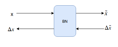
We first consider the simplest case where a layer consists of the BN operation only. We use ${\bf x}$ and ${\tilde{\bf x}}$ to denote a batch of input and output values to and from a batch normalized (BN) layer, respectively. The standard normal variate of ${\bf x}$ is ${\bf z}$ i.e. the vector ${\bf z}$ is calculated by element wise normalization of input batch ${\bf x}$. In gradient backpropagation, the batch of input gradient values to the BN layer is $\Delta{\tilde{\bf x}}$ while the batch of output gradient values from the BN layer is $\Delta{\bf x}$. Mathematically, we have

$$\tilde{\bf x}=BN({\bf x})$$ (3)

By simple manipulation of the formulas given in Ioffe and Szegedy (2015), we can get

$$\Delta{x_{i}}=\frac{\gamma}{Std(x_{i})}((\Delta{\tilde{x}_{i}}-E(\Delta{\tilde{x}_{i}}))-z_{i}E(\Delta{\tilde{x}_{i}}z_{i})),$$ (4)

where $x_{i}$ is the $i$th feature of ${\bf x}$ and $Std()$ is the standard deviation of element $x_{i}$ across the batch. Then, it is straightforward to derive

$$E(\Delta{x}_{i})=0,\quad\mbox{and}\quad Var(\Delta{x}_{i})=\frac{\gamma^{2}}{Var(x_{i})}(Var(\Delta\tilde{x}_{i})-(E(\Delta\tilde{x}_{i}z_{i}))^{2}).$$ (5)

Figure 1: Illustration of a BN layer.

3.2 Cascaded BN/ReLU/CONV Layer

Next, we examine a more complex but common case, where a layer consists of three operations in cascade. They are: 1) batch normalization, 2) ReLU activation, and 3) convolution. Here, we take BN and ReLU before convolution because we want to explore the activation of a convolution layer by taking the layer input activation into consideration. It doesn’t matter whether BN and ReLU are actually placed before or after convolution, because if they are actually placed after a convolution layer, we can consider our calculations taking them as placed before the next convolution layer. To simplify the gradient flow calculation, we make some assumptions which will be mentioned whenever needed.

The input to the $L$th Layer of a deep neural network is ${\bf y}_{L-1}$ while its output is ${\bf y}_{L}$. We use $BN$, $ReLU$ and $CONV$ to denote the three operations in each sub-layer. Then, we have the following three equations:

$$\tilde{\bf y}_{L-1}=BN({\bf y}_{L-1}),\quad\hat{\bf y}_{L-1}=ReLU(\tilde{\bf y}_{L-1}),\quad{\bf y_{L}}=CONV(\hat{\bf y}_{L-1}).$$ (6)

The relationship between ${\bf y}_{L-1}$, $\tilde{\bf y}_{L-1}$, $\hat{\bf y}_{L-1}$ and ${\bf y}_{L}$ is shown in Fig. 2. As shown in the figure, $\tilde{\bf y}_{L-1}$ denotes the batch of output elements from the BN sub-layer. It also serves as the input to the ReLU sub-layer. $\hat{\bf y}_{L-1}$ denotes the batch of output elements from the ReLU sub-layer. It is fed into the convolution sub-layer. Finally, ${\bf y}_{L}$ is the batch of output elements from the CONV sub-layer. Gradient vectors have $\Delta$ as the prefix to their corresponding vectors in the forward pass. In this figure, ${\bf W}_{L}$ is the weight vector of the convolution layer. The dimensions of ${\bf y}_{L}$ and $\Delta{\bf y}_{L}$ are $n_{L}$ and $n_{L}^{\prime}$, respectively. $y_{L-1,i}$ denotes the $i$th feature of activation ${\bf y}_{L-1}$.

Figure 2: Illustration of a layer that consists of BN, ReLU and CONV three sub-layers.

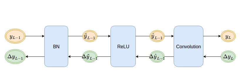
Please note that from now on in the derived equations, $Var(y_{L})$ denotes a vector, where each element $Var(y_{L,i})$ denotes the variance of element $y_{L,i}$ across its batch. $Var(W_{L,.})$ denotes the variance of the entire weight matrix. To simplify representation, we denote $W^{2}$ as the element wise squared matrix of W. Also, $W^{T}$ denotes the transpose of matrix W.

3.2.1 Variance Analysis in Forward Pass

We will derive the mean and variance of output $y_{L,i}$ from the input ${\bf y}_{L-1}$. First, we examine the effect of the BN sub-layer. The output of a batch normalization layer is $\gamma_{i}z_{i}+\beta_{i}$, where $z_{i}$ is the standard normal variate of $y_{L-1,i}$, calculated across a batch of activations. Clearly, we have

$$E(\tilde{y}_{L-1,i})=\beta_{i},\quad\mbox{and}\quad Var(\tilde{y}_{L-1,i})=\gamma_{i}^{2}.$$ (7)

Next, we consider the effect of the ReLU sub-layer. Let $a=\frac{\beta_{i}}{\gamma_{i}}$. In Appendix A, we show a step-by-step procedure to derive the mean and variance of the output of the ReLU sub-layer when it is applied to the output of a BN layer. Here, we summarize the main results below:

$$E(\hat{y}_{L-1,i}) = \gamma_{i}\left(\frac{1}{\sqrt{2\pi}}+\frac{a}{2}+\frac{1}{\sqrt{2\pi}}(1-\exp(\frac{-a^{2}}{2}))\right)$$ (8)

$$E(\hat{y}_{L-1,i}^{2}) = E(y^{2})=0.5+\sqrt{\frac{2}{\pi}}a+0.5a^{2}+\exp(\frac{-a^{2}}{2})+p(a)$$ (9)

where p(a) = $\int_{0}^{a}\frac{1}{\sqrt{2\pi}}\exp(\frac{-z^{2}}{2})dz$.

Finally, we consider the influence of the CONV sub-layer. $W_{L}$ is the matrix of the CONV sub-layer of dimension ($n_{L}^{\prime},n_{L}$) i.e. $(y_{L})_{n_{L}^{\prime}*1}$ = $(W_{L})_{n_{L}^{\prime}*n_{L}}$ $(\hat{y}_{L-1})_{n_{L}*1}$. Here, we assume that all elements in ${\bf\hat{y}}_{L-1}$ are mutually independent. Then, it’s trivial to see that since we are calculating the variance across a batch of activations,

$$Var(y_{L})=W_{L}^{2}Var(\hat{y}_{L-1})$$ (10)

3.2.2 Variance Analysis in Backward Pass

We consider backward propagation from the $L$th layer to the $(L-1)$th layer and focus on gradient propagation. Since, the gradient has just passed through the BN sub-layer of Lth layer, using eq. (5) we get E($\Delta{\bf y}_{L}$) = 0. Note that here 0 denotes the vector 0 in dimension of length of $y_{L}$.

First, gradients go through the CONV sub-layer. $(\Delta{\hat{y}}_{L-1})_{n_{L}*1}$ = $(W_{L}^{T})_{n_{L}*n_{L}^{\prime}}$ $(\Delta{y}_{L})_{n_{L}^{\prime}*1}$. Here, we assume that all elements in ${\bf\Delta{y}}_{L}$ are mutually independent. Then, it’s trivial to see that since we are calculating the expectation and variance across a batch of activations,

$$E(\Delta{\hat{y}}_{L-1})=W_{L}^{T}E(\Delta{\bf y}_{L})=0\mbox{ and }Var(\Delta{\hat{y}}_{L-1})=(W_{L}^{T})^{2}Var(\Delta{y}_{L})$$ (11)

Next, gradients go through the ReLU sub-layer. It is assumed that the function applied to the gradient vector on passing through ReLU and the elements of gradient are independent of each other. Since the input in the forward pass was a shifted normal variate ($a=\frac{\beta_{i}}{\gamma_{i}}$), we get

$$E(\Delta\tilde{y}_{L-1,i})=(0.5+p(a))E(\Delta{\hat{y}_{L-1,i}})=0.0,\mbox{ and }$$ (12)

$$Var(\Delta\tilde{y}_{L-1,i})=(0.5+p(a))Var(\Delta{\hat{y}_{L-1,i}}).$$

where p(a) = $\int_{0}^{a}\frac{1}{\sqrt{2\pi}}\exp(\frac{-z^{2}}{2})dz$.

In the final step, gradients go through the BN sub-layer. If the standard normal variate, ${\bf z}$, to the BN sub-layer and the incoming gradients $\Delta{\bf y}$ are independent, we have $E(z_{i}\Delta y_{L-1,i})=E(z_{i})E(\Delta y_{L-1,i})=0$. The last equality holds since the mean of the standard normal variate is zero.

The final result is

$$Var(\Delta y_{L-1,i})=\frac{\sum_{j=1}^{n_{L}^{\prime}}W_{L,ji}^{2}Var(\Delta y_{L,j})}{\sum_{j=1}^{n_{L-1}}W_{L-1,ij}^{2}}\frac{0.5+p(a)}{0.5+\sqrt{\frac{2}{\pi}}a+0.5a^{2}+\exp(\frac{-a^{2}}{2})+p(a)}$$ (13)

.

where p(a) = $\int_{0}^{a}\frac{1}{\sqrt{2\pi}}\exp(\frac{-z^{2}}{2})dz$

Let’s see what the above equation means. The numerator shows a weighted sum of the gradient elements of Lth layer, the weights being the ith column of weight matrix $W_{L}$. While the denominator shows a simple summation of the ith row of weight matrix $W_{L-1}$. Now, we take some assumptions to simplify the above equation, derive some meaning of the above equation and find the expectation of gradient vector $y_{L}$. To simplify the analysis, we assume that all elements in ${\bf W}_{L}$ are of the same distribution of mean 0. All elements in Var($\Delta y_{L-1}$) are from the same distribution. Furthermore, Var($\Delta y_{L-1}$) and ${\bf W}_{L}$ are independent of each other. Also, I assume that the weight variables are bounded i.e. they don’t increase indefinitely. This is a fair assumption and this is required to show that

$$E(\frac{1}{X})E(X)\leq\frac{(c+d)^{2}}{4cd}$$

where X is a variable and lies in the range (c,d), $0<c<d$. Also, for the same variable X, since $\frac{1}{X}$ is convex function,

$$E(\frac{1}{X})E(X)\geq 1$$

Using the above properties and assumptions, we get,

$$\frac{n_{L}^{\prime}}{n_{L-1}}\frac{Var(W_{L})}{Var(W_{L-1})}E(Var(\Delta y_{L,i})) \leq E(\frac{\sum_{j=1}^{n_{L}^{\prime}}W_{L,ji}^{2}Var(\Delta y_{L,j})}{\sum_{j=1}^{n_{L-1}}W_{L-1,ij}^{2}})$$

$$\leq K\frac{n_{L}^{\prime}}{n_{L-1}}\frac{Var(W_{L})}{Var(W_{L-1})}E(Var(\Delta y_{L,i}))$$

where we assume that K is a constant such that when X = $\sum_{j=1}^{n_{L-1}}W_{L-1,ij}^{2}$ i.e. sum of a row of matrix $W_{L-1}^{2}$, the upper bound on $E(\frac{1}{X})\leq\frac{K}{E(X)}$ holds. Thus,

$$E(Var(\Delta y_{L,i}))\frac{n_{L}^{\prime}}{n_{L-1}}\frac{Var(W_{L,.})}{Var(W_{L-1,.})}\frac{0.5+p(a)}{0.5+\sqrt{\frac{2}{\pi}}a+0.5a^{2}+\exp(\frac{-a^{2}}{2})+p(a)}\leq E(Var(\Delta y_{L-1,i}))$$ (14)

$$\leq KE(Var(\Delta y_{L,i}))\frac{n_{L}^{\prime}}{n_{L-1}}\frac{Var(W_{L,.})}{Var(W_{L-1,.})}\frac{0.5+p(a)}{0.5+\sqrt{\frac{2}{\pi}}a+0.5a^{2}+\exp(\frac{-a^{2}}{2})+p(a)}$$

where p(a) = $\int_{0}^{a}\frac{1}{\sqrt{2\pi}}\exp(\frac{-z^{2}}{2})$.

Note that the last product term in the upper and lower bound is a constant term. The other two fractions are properties of the network, that compare two adjacent Layers. Also, assuming that the weights come from a distribution of mean 0 is a valid assumption because a) the weights are initialized with 0 mean and b) the gradients that come to the convolution layer have mean 0 by eq (5) across batch. The skipped steps are given in Appendix B.

3.3 Discussion

Initially, we set $\beta_{i}=0$ and $\gamma_{i}=1$ so that $a=0$. Then, the constant term in the RHS of Eq. (13) is equal to one. Hence, if the weight initialization stays equal across all the layers, propagated gradients are maintained throughout the network. In other words, the BN simplifies the weight initialization job. For intermediate steps, we can estimate the gradient variance under simplifying assumptions that offer a simple minded view of gradient propagation. Note that, when $a=\frac{\beta}{\gamma}$ is small (the experimental values of a in fig 14 show that it reaches at most 1.0), the constant term is a reasonable constant (at a=1.0, the constant is around 0.33 and as the value of a decreases to 0.0, the constant approaches 1.0). The major implication is that, the BN helps maintain gradients across the network, throughout the training, thus stabilizing optimization.

4 Gradient Propagation Through A Resnet Block

4.1 Resnet Block

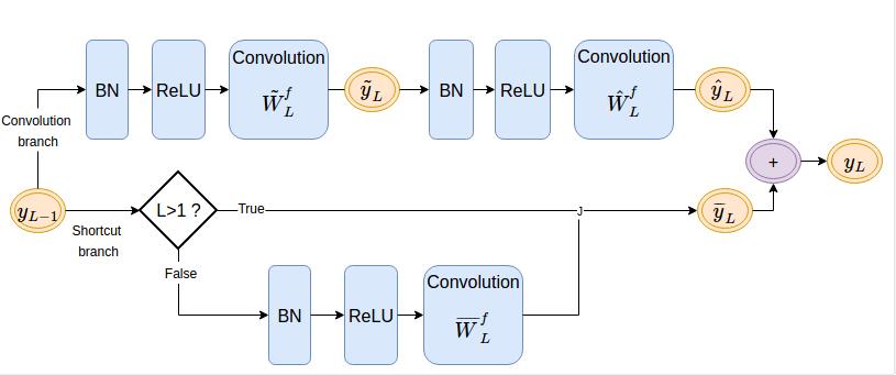
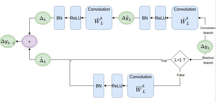
The resnet blocks in the forward pass and in the gradient backpropagation pass are shown in Figs. 3 and 4, respectively. A residual network has multiple scales, each scale has a fixed number of residual blocks, and the convolutional layer in residual blocks at the same scale have the same number of filters. In the analysis, we adopt the model where the filter number increases $k$ times from one scale to the next one. Although no bottleneck blocks are explicitly considered here, our analysis holds for bottleneck blocks as well. As shown in Fig. 3, the input passes through a sequence of BN, ReLU and CONV sub-layers along the shortcut branch in the first residual block of a scale, which shapes the input to the required number of channels in the current scale. For all other residual blocks in the same scale, the input just passes through the shortcut branch. For all residual blocks, the input goes through the convolution branch which consists of two sequences of BN, ReLU and CONV sub-layers. We use a layer to denote a sequence of BN, ReLU and CONV sub-layers as used in the last section and $F$ to denote the compound function of one layer. Note that in the first residual block, we use an explicit BN sub layer in the shortcut branch. However, in the current resnet models, the BN sublayer and ReLU sublayer are used before the residual block. The calculations won’t change, if we use individual BN+ReLU in each branch but the representation is simple.

Figure 3: A residual block in the forward pass.

Figure 4: A residual block in the gradient backpropagation pass.

To simplify the computation of the mean and variance of $y_{L,i}$ and $\Delta{y_{L,i}}$, we assume that $a=\frac{\beta_{i}}{\gamma_{i}}$. is a constant. We can always take a as the average across the layers. We define the following two associated constants.

$$c_{1} = 0.5+p(a)$$ (15)

$$c_{2} = 0.5+\sqrt{\frac{2}{\pi}}a+0.5a^{2}+p(a)+exp(\frac{-a^{2}}{2})$$ (16)

where p(a) = where p(a) = $\int_{0}^{a}\frac{1}{\sqrt{2\pi}}\exp(\frac{-z^{2}}{2})dz$.

which will be needed later. We show the results for the upper bound. The lower bound is just a factor smaller than the upper bound.

4.2 Variance Analysis

As shown in Fig. 3, block $L$ is the $L$th residual block in a scale with its input $y_{L-1}$ and output $y_{L}$. The outputs of the first and the second BN-ReLU-CONV layers in the convolution branch are $\tilde{y}_{L}=F(y_{L-1})$ and $\hat{y}_{L}=F(F(y_{L-1}))$, respectively. The weight vectors of the CONV sub-layer of the first and the second layers in the convolution branch of block $L$ are $\tilde{W}_{L}$ and $\hat{W}_{L}$, respectively. The weight vector in the shortcut branch of the first block is $\overline{W}_{1}$. The output of the shortcut branch is $\overline{y}_{L}$. For $L=1$, we have $\overline{y}_{1}=F(y_{0})$, where $y_{0}$ is the output of last residual block of the previous scale. For L$>$1, we have $\overline{y}_{L}=y_{L-1}$. For the final output, we have

$$y_{L}=\overline{y}_{L}+\hat{y}_{L}.$$ (17)

For L$>$1, block $L$ receives an input of size $n_{s}$ in the forward pass and an input gradient of size $n_{s}^{\prime}$ in the backpropagation pass. Since block $1$ receives its input $y_{0}$ from the previous scale, it receives an input of size $\frac{n_{s}}{k}$ in the forward pass.

By assuming $\overline{y}_{L}$ and $\hat{y}_{L}$ are independent, we have

$$Var(y_{L,i})=Var(\overline{y}_{L,i})+Var(\hat{y}_{L,i}).$$ (18)

We will show how to compute the variance of $y_{L,i}$ step by step in Appendix C for $L=1,\cdots,N$. When $L=N$, we obtain

$$Var(y_{N})=c_{2}(\sum_{J=2}^{N}\hat{W}_{J}^{2}I_{n_{J}}+\frac{1}{k}(\overline{W}_{1}^{2}I_{n_{1}}+\hat{W}_{1}^{2}I_{n_{1}}))$$ (19)

where $c_{2}$ is defined in Eq. (16) and $I_{x}$ denotes a one vector of dimension x.

We use $\Delta$ as prefix in front of vector representations at the corresponding positions in forward pass to denote the gradient in Fig. 4 in the backward gradient propagation. Also, as shown in Fig. 4, we represent the gradient vector at the tip of the convolution branch and shortcut branch by $\Delta_{L}$ and $\hat{\Delta}_{L}$ respectively. As shown in the figure, we have

$$\Delta y_{L-1}=\hat{\Delta}_{L}+\Delta_{L}$$ (20)

A step-by-step procedure in computing the variance of $\Delta{y_{L-1,i}}$ is given in Appendix D. Here, we show the final result below:

$$E(Var(\Delta{y_{L-1,i}}))\leq K_{L} \left(1+(\frac{c_{1}}{c_{2}})^{2}\frac{Var(\tilde{W}_{L,.})}{\sum_{J=2}^{L-1}Var(\hat{W}_{J,.})+\frac{1}{k}(Var(\overline{W}_{1,.})+Var(\hat{W}_{1,.}))}\right)$$ (21)

$$E(Var(\Delta{y_{L,i}})).$$

where $K_{L}$ denotes the necessary bound of the convolution layers in residual block L, as used in eq(14).

4.3 Discussion

We can draw two major conclusions from the analysis conducted above. First, it is proper to relate the above variance analysis to the gradient vanishing and explosion problem. The gradients go through a BN sub-layer in one residual block before moving to the next residual block. As proved in Sec. 3, the gradient mean is zero when it goes through a BN sub-layer and it still stays at zero after passing through a residual block. Thus, if it is normally distributed, the probability of the gradient values between $\pm$ 3 standard deviations is 99.7%. A smaller variance would mean lower gradient values. In contrast, a higher variance implies a higher likelihood of discriminatory gradients. Thus, we take the gradient variance across a batch as a measure for stability of gradient backpropagation.

Second, recall that the number of filters in each convolution layer of a scale increases by $k$ times with respect to its previous scale. Typically, $k=1$ or $2$. Without loss of generality, we can assume the following: the variance of weights is about equal across layers, ${c_{1}}/{c_{2}}$ is a reasonably small constant, and $k=2$. Then, Eq. (21) can be simplified to

$$Upperbound(E(Var(\Delta{y_{L-1,i}})))\propto K_{L}\frac{L}{L-1}E(Var(\Delta{y_{L,i}})).$$ (22)

We see from above that the change in the gradient variance from one residual block to its next is small. This is especially true when the $L$ value is high. Thus, the gradient variance increases as we move across a scale. This observation can be used to explain the iterative estimation given in Greff et al. (2016). The gradient variance is high in the lower blocks in a scale, while it is low in the upper blocks. That shows a vigorous change in weights in the lower blocks and the weight change gets finer as we move forward. Hence, the weights in the upper blocks are smoothly refined so that the features learned in the lower blocks gets finer as we move forward towards the upper blocks of a scale.

4.4 Experimental Verification

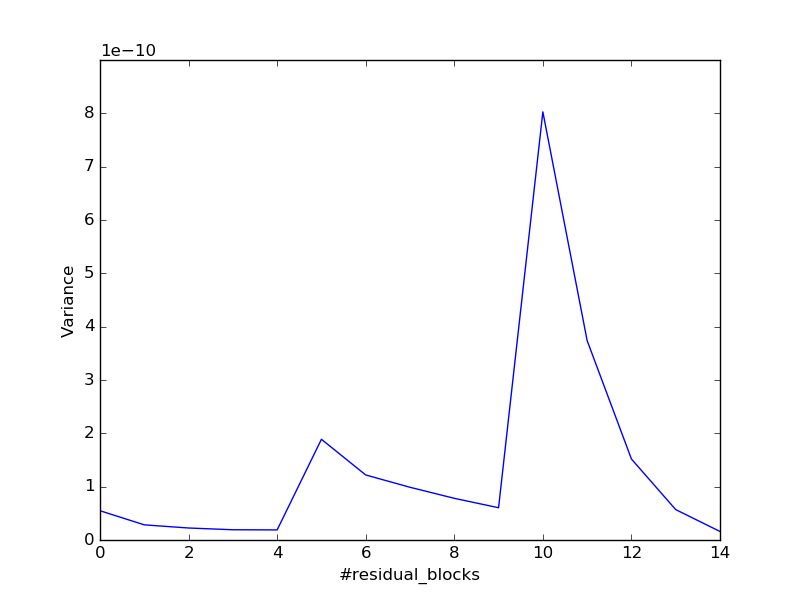
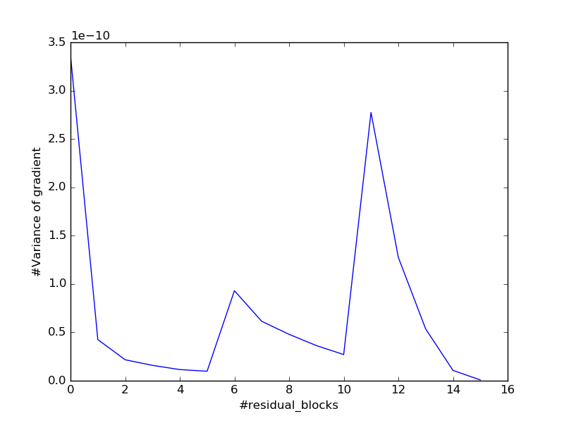
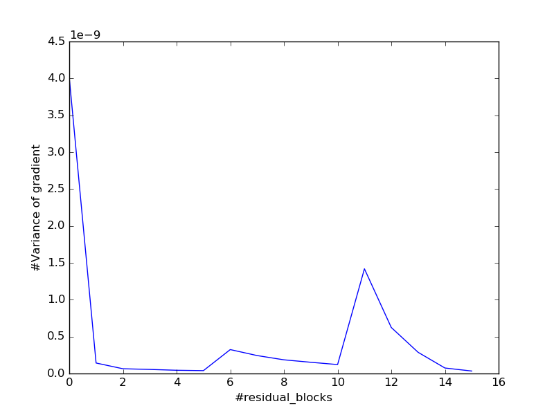
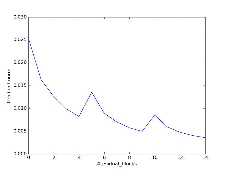
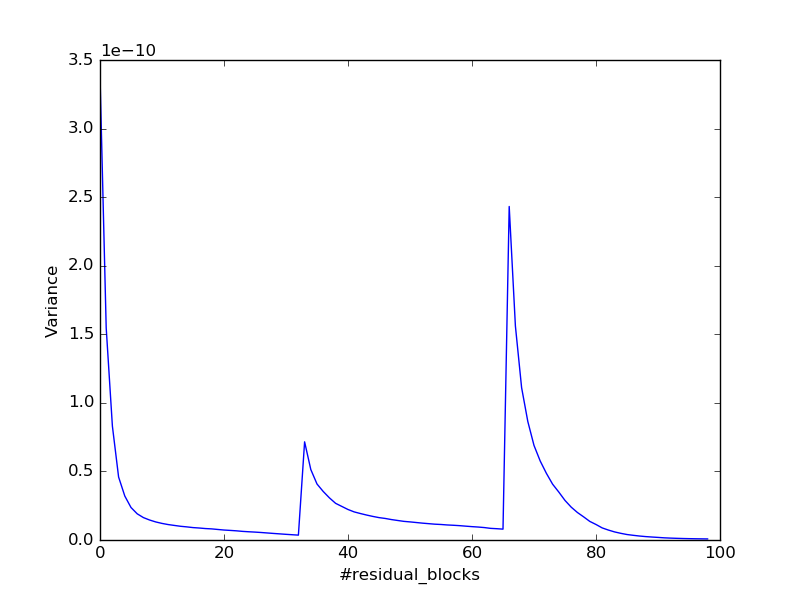
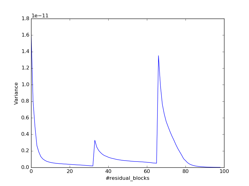
We trained a Resnet-15 model that consists of 15 residual blocks and 3 scales on the CIFAR-10 dataset, and checked the gradient variance across the network throughout the training. We plot the mean of the gradient variance and the $l_{2}$-norm of the gradient at various residual block locations in Figs. 5 and 6, respectively, where the gradient variance is calculated for each feature across one batch. Since gradients backpropagate from the output layer to the input layer, we should read each plot from right to left to see the backpropagation effect. The behavior is consistent with our analysis. There is a gradual increase of the slope across a scale. The increase in the gradient variance between two residual blocks across a scale is inversely proportional to the distance between the residual blocks and the first residual block in the scale. Also, there is a dip in the gradient variance value when we move from one scale to its previous scale. Since the BN sub-layer is used in the shortcut branch of the first block of a scale, it ensures the decrease of the gradient variance as it goes from one scale to another.

Figure 5: The mean of the gradient variance as a function of the residual block position at Epoch 1 (left), Epoch 25000 (middle) and Epoch 50000 (right).

Figure 6: The $l_{2}$ norm of the gradient as a function of the residual block position at Epoch 1 (left), Epoch 25000 (middle) and Epoch 50000 (right).

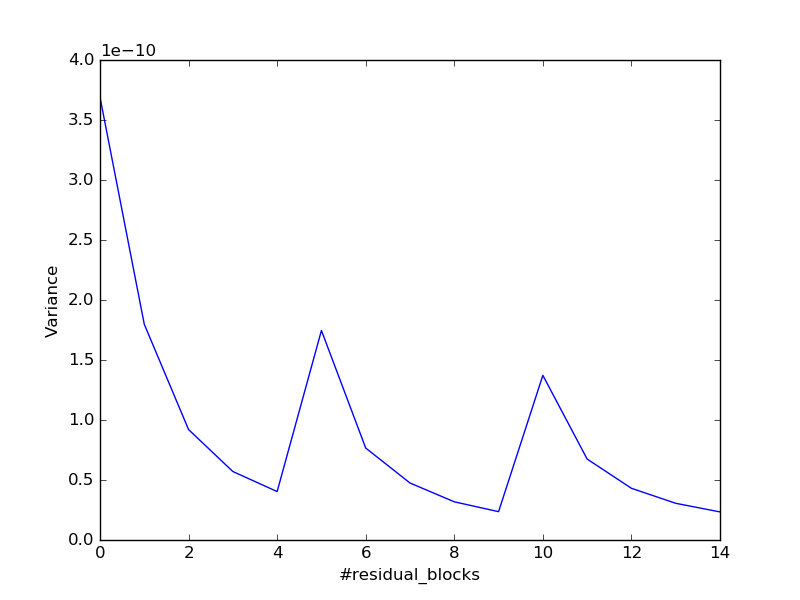
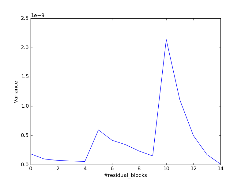
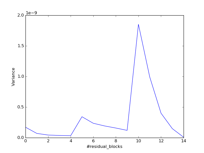
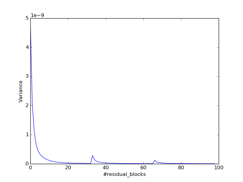
We observed similar results in case of Resnet-99, where the number of residual networks in each scale is 33. The results are shown in Fig(7).

Figure 7: The mean of the gradient variance as a function of the residual block position at Epoch 1 (left), Epoch 25000 (middle) and Epoch 50000 (right) in case of resnet-99.

5 Batch normalization vs residual branch in resnet

We analysed the importance of batch normalization in resnet in the previous section. However, there is one question that needs to be solved, the relative importance of batch normalization w.r.t. the residual branches. We compared two variations of residual network with the original model. The models were trained on CIFAR-10. The models compared were

• Model-1: Residual network with BN and residual branches

• Model-2: Residual network with BN only (residual branches have been removed)

• Model-3: Residual network with residual branches only (BN layers have been removed)

Figure 8: Comparison of training accuracy for Model-1(red), Model-2(violet) and Model-3 (blue).

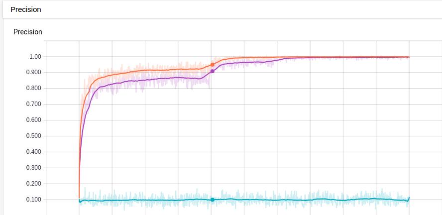
All the models had 15 residual blocks, 5 in each scale. The parameters of each model were initialized similarly and were trained for same number of epochs. The weights were initialized with xavier initialization and the biases were initialized to 0. First, we compare the training accuracy among the three models in Fig. 8, where the horizontal axis shows the epoch number. We see that Model-1 reaches higher accuracy faster than the other two models. However, Model-2 isn’t far behind. But Model-3, which has BN removed, doesn’t learn anything. Next, we compare their test set accuracy in Table 1. We see that Model-1 has the best performance while Model-2 isn’t far behind.

Model	Final accuracy
Model-1	92.5%
Model-2	90.6%
Model-3	9.09%

Table 1: Comparison of test accuracy of three Resnet models.

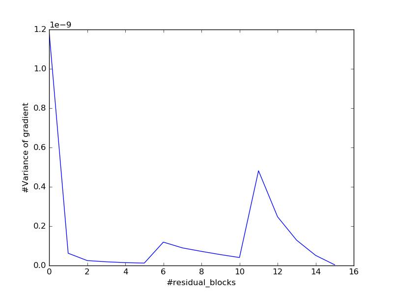
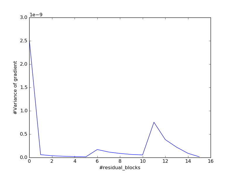
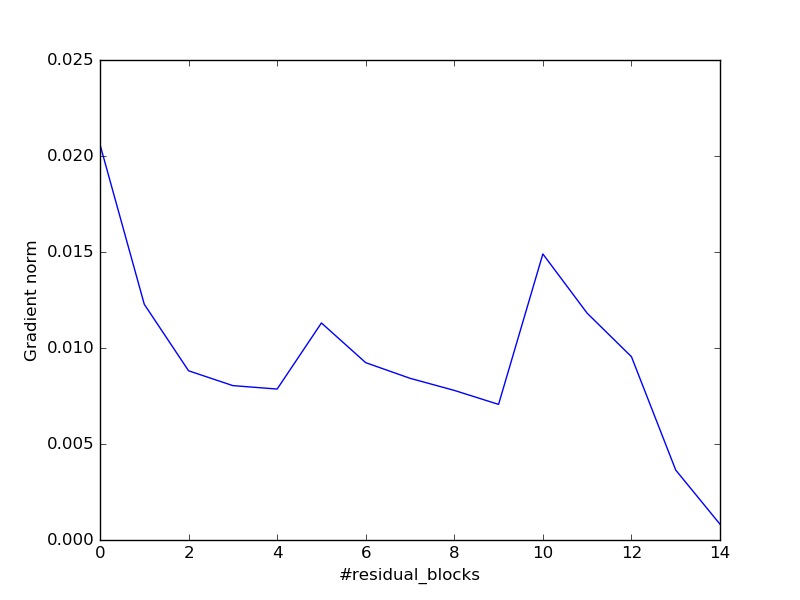
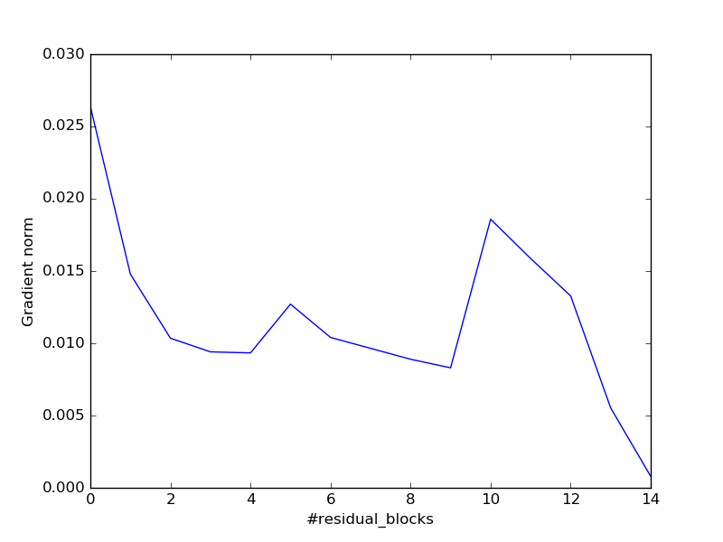
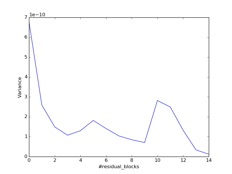
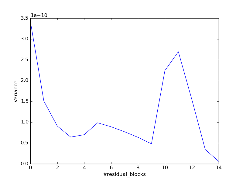
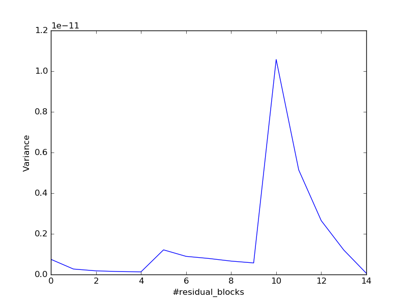
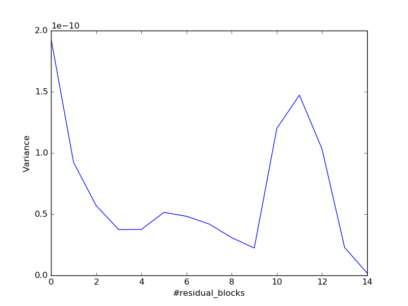
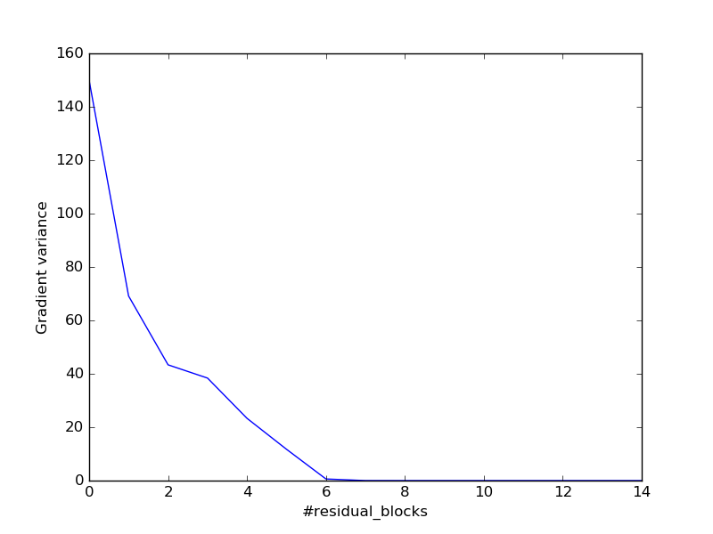
Furthermore, we plot the mean of the gradient variance, calculated for each feature across one batch, as a function of the residual block index at epochs 25,000, 50,000 and 75,000 in Figs. 9, 10 and 11, respectively, where the performance of Model-1 and Model-2 is compared. We observe that the gradient variance also stays within a certain range, without exploding or vanishing, in case of Model-2. However, the change in gradient variance across a scale doesn’t follow a fixed pattern compared to Model-1. We also plot a similar kind of plot for Model-3 at epoch-1 in Fig 12. We observed gradient explosion, right from the start, in case of Model-3 and the loss function had quickly become undefined. This was the reason, why Model-3 didn’t learn much during the course of training.

This experiment shows that BN plays a major role in stabilizing training of residual networks. Even though we remove the residual branches, the network still tries to learn from the training set, with its gradient fixed in a range across layers. However, removing BN hampers the training process right from the start. Thus, we can see that batch normalization helps to stop gradient vanishing and explosion throughout training, thus stabilizing optimization. Thus, the success of residual networks can’t be attributed only to residual branches. Both BN and residual branches are responsible for the success of residual networks.

Figure 9: The gradient variance as a function of the residual block index during backpropagation in Model-1 (left), and Model-2 (right) at Epoch 25000.

Figure 10: The gradient variance as a function of the residual block index during backpropagation in Model-1 (left), and Model-2 (right) at Epoch 50000.

Figure 11: The gradient variance as a function of the residual block index during backpropagation in Model-1 (left), and Model-2 (right) at Epoch 75000.

Figure 12: Gradient explosion observed during back propagation in Model-3 at epoch-1

6 Conclusion and Future Work

Batch normalization (BN) is critical to the training of deep residual networks. Mathematical analysis was conducted to analyze the BN effect on gradient propagation in residual network training in this work. We explained how BN and residual branches work together to maintain gradient stability across residual blocks in back propagation. As a result, the gradient does not explode or vanish in backpropagation throughout the whole training process. We also showed experimentally the relative importance of batch normalization w.r.t the residual branches and showed that BN is important for stopping gradient explosion during training.

The Saak transform has been recently introduced by Kuo and Chen (2017), which provides a brand new angle to examine deep learning. The most unique characteristics of the Saak transform approach is that neither data labels nor backpropagation is needed in training the filter weights. It is interesting to study the relationship between multi-stage Saak transforms and residual networks and compare their performance in the near future.

7 References

Appendix A

We apply the ReLU to the output of a BN layer, and show the step-by-step procedure in calculating the variance and the mean of the output of the ReLU operation. In the following derivation, we drop the layer and the element subscripts (i.e., $L$ and $i$) since there is no confusion. Let $a=\beta/\gamma$. Then, we can write the shifted Gaussian variate due to the BN operation as

$$\gamma z+\beta=\gamma(z+a).$$ (23)

Let $y=ReLU(z+a)$. Let a $>$ 0. We can write

$$E(y)= P(z<-a)E(y|z<-a)+P(-a<z<0)E(y|-a<z<0)$$ (24)

$$+P(z>0)E(y|z>0).$$

The first right-hand-side (RHS) term of Eq. (24) is zero since $y=0$ if $z<-a$ due to the ReLU operation. Thus, $E(y|z<-a)=0$. For the second RHS term, we have

$$P(0<z<a)=\int_{0}^{a}\frac{1}{\sqrt{2\pi}}\exp(\frac{-z^{2}}{2})dz$$

$$E(y;-a<z<0)=\int_{0}^{a}z\frac{1}{\sqrt{2\pi}}\exp(\frac{-z^{2}}{2})dz=\frac{1}{\sqrt{2\pi}}(1-\exp(\frac{-a^{2}}{2}))$$ (25)

For the third RHS term, $P(z>0)=0.5$. Besides, $z>0$ is half-normal distributed. Thus, we have

$$E(y|z>0)=E(|z|)+a=\sqrt{\frac{2}{\pi}}+a$$ (26)

Based on the above results, we get

$$E(y)=\frac{1}{\sqrt{2\pi}}+\frac{a}{2}+\frac{1}{\sqrt{2\pi}}(1-\exp(\frac{-a^{2}}{2}))$$ (27)

Similarly, we can derive a formula for $E(y^{2})$ as

$$E(y^{2}) = P(z<-a)E(y^{2}|z<-a)+P(-a<z<0)E(y^{2}|-a<z<0)$$ (28)

$$+P(z>0)E(y^{2}|0<z<a).$$

For the first RHS term of Eq. (28), we have $E(y^{2}|z<-a)=0$ due to the ReLU operation. For the second RHS term of Eq. (28),

$$E(y^{2};-a<z<0)=\int_{0}^{a}z^{2}\frac{1}{\sqrt{2\pi}}\exp(\frac{-z^{2}}{2})dz=\frac{-a}{\sqrt{2\pi}}\exp(\frac{-a^{2}}{2})-\int_{0}^{a}\frac{1}{\sqrt{2\pi}}\exp(\frac{-z^{2}}{2})dz$$

For the third RHS term $P(z>0)=0.5$ for $z>0$. The random variable $z>0$ is half normal distributed so that

$$\begin{aligned} E(y^{2}|z>0)=&E((|z|+a)^{2})=E(|z|^{2})+a^{2}+2aE(|z|)\\ &=a^{2}+2\sqrt{\frac{2}{\pi}}a+1.\end{aligned}$$ (29)

Then, we obtain

$$E(y^{2})=0.5+\sqrt{\frac{2}{\pi}}a+0.5a^{2}+\exp(\frac{-a^{2}}{2})+p(a)$$ (30)

where p(a) = $\int_{0}^{a}\frac{1}{\sqrt{2\pi}}\exp(\frac{-z^{2}}{2})dz$.

We can follow the same procedure for $a<0$. The final results are summarized below.

$$E(ReLU(\gamma z+\beta))=\gamma E(y)\quad\mbox{and}\quad E((ReLU(\gamma z+\beta))^{2})=\gamma^{2}E(y^{2}),$$ (31)

where $E(y)$ and $E(y^{2})$ are given in Eqs. (27) and (30), respectively.

Appendix B

• We assumed that the function(F) applied by ReLU to the gradient vector and the gradient elements are independent of each other. Function F is defined as

  $$F(\Delta{y})=\Delta{y}I_{y>0}$$

  where $\Delta{y}$ denotes input gradient in gradient backpropagation and y denotes the input activation during forward pass to the ReLU layer. $I_{y>0}$ = 1 when y$>$0 and it is 0 otherwise. Coming back to our analysis, since $\tilde{y}_{L-1,i}$ is a normal variate shifted by $a$, the probability that the input in forward pass to the ReLU layer, i.e. $\tilde{y}_{L-1,i}$ is greater than 0 is

  $$P(\tilde{y}_{L-1,i}>0)=0.5+p(a).$$

  where p(a) = $\int_{0}^{a}\frac{1}{\sqrt{2\pi}}\exp(\frac{-z^{2}}{2})dz$.

  Thus, E(F($\Delta{\hat{y}}_{L-1,i}$)) = E($\Delta{\hat{y}}_{L-1,i}$) P($\tilde{y}_{L-1,i}>0$), and so

  $$E(\Delta{\tilde{y}}_{L-1,i})=(0.5+p(a))\mbox{ }E(\Delta{\hat{y}}_{L-1,i})$$

  Similarly, we can solve for Var($\Delta{\tilde{y}}_{L-1,i}$) and thus, get Eq. (12).

• First, using eq 5 and the assumption that the input standard normal variate in forward pass and the input gradient in gradient pass are independent, we have

  $$Var(\Delta y_{L-1,i}) = \frac{\gamma_{i}^{2}}{Var(y_{L-1,i})}Var(\Delta{\tilde{y}_{L-1,i}})$$ (32)

  $$= \frac{\gamma_{i}^{2}}{Var(y_{L-1,i})}(0.5+p(a))\sum_{j=1}^{n_{L}^{\prime}}W_{L,ji}^{2}Var(\Delta y_{L,j}).$$ (33)

  where p(a) = $\int_{0}^{a}\frac{1}{\sqrt{2\pi}}\exp(\frac{-z^{2}}{2})dz$.

  Then, using Eq. (10) for $Y_{L-1}$ (yet with $L$ replaced with $L-1$), we can get Eq. (13).

Appendix C

For $L=1$, $\overline{y}_{1}=F(y_{0})$. Let $I_{x}$ denote a one vector of dimension x. Since the receptive field for the last scale is $k$ times smaller, we get the following from Eq. (10),

$$Var(\overline{y}_{1})=c_{2}\overline{W}_{1}^{2}I_{n_{1}}$$ (34)

Also, since $\hat{y}_{1}=F(F(y_{0}))$, we have

$$Var(\hat{y}_{1})=c_{2}\hat{W}_{1}^{2}I_{n_{1}}$$

based on Eq. (10). Therefore, we get

$$Var(y_{1}) = c_{2}(\overline{W}_{1}^{2}I_{n_{1}}+\hat{W}_{1}^{2}I_{n_{1}})$$ (35)

For $L=N>1$, the input just passes through the shortcut branch. Then,

$$Var(\overline{y}_{N,i})=Var(y_{N-1,i})$$

Also, since $\hat{y}_{N}=F(F(y_{N-1}))$, we have

$$Var(\hat{y}_{N})=c_{2}\hat{W}_{N}^{2}I_{n_{N-1}}$$

due to using Eq. (10). Thus,

$$Var(y_{N})=Var(y_{N-1})+c_{2}\hat{W}_{N}^{2}I_{n_{N-1}}$$ (36)

Doing this recursively from $L=1$ to $N$, we get

$$Var(y_{N})=c_{2}(\sum_{J=2}^{N}\hat{W}_{J}^{2}I_{n_{J}}+\overline{W}_{1}^{2}I_{n_{1}}+\hat{W}_{1}^{2}I_{n_{1}})$$ (37)

Appendix D

Let $\tilde{K}_{L}$ and $\hat{K}_{L}$ denote the necessary upperbound for the convolution layer weights in the convolution branch, as needed by eq(14).

For block $L=N>1$, the gradient has to pass through two BN-ReLU-Conv Layers in convolution branch. Since, the receptive field doesn’t change in between the two BN-ReLU-Conv Layers in the convolution branch of the block, we use Eq. (13) and find that for same receptive field between the two layers i.e. $n_{L}$ $=$ $n_{L-1}^{\prime}$ ,

$$E(Var(\Delta{\tilde{y}_{L,i}}))\leq\hat{K}_{L}\frac{c_{1}}{c_{2}}\frac{Var(\hat{W}_{L,.})}{Var(\tilde{W}_{L,.})}E(Var(\Delta{y}_{L,i})).$$ (38)

When gradient passes through the first BN-ReLU-Conv Layer, the variance of the forward activation that BN component sees is actually the variance of the output of previous block. Hence, using Var($y_{L-1,i}$), which is the output of previous residual block, in place of the denominator in Eq. (32), we get

$$E(Var(\Delta_{L,i}))\leq \tilde{K}_{L}\frac{c_{1}}{c_{2}}\frac{Var(\tilde{W}_{L,.})}{\sum_{J=2}^{L-1}Var(\hat{W}_{J,.})+\frac{1}{k}(Var(\overline{W}_{1,.})+Var(\hat{W}_{1,.}))}$$ (39)

$$E(Var(\Delta{\tilde{y}_{L,i}}))$$

We assume that $\hat{\Delta}_{L}$ and $\Delta_{L}$ are independent of each other. Since we are calculating for Block L$>$1 where there is no BN-ReLU-Conv Layer in shortcut branch, we have $Var(\hat{\Delta}_{L,i})=Var(\Delta{y_{L,i}})$. As,

$$E(Var(\Delta{y_{L-1,i}}))=E(Var(\Delta_{L,i}))+E(Var(\hat{\Delta}_{L,i})).$$

Finally, we obtain

$$E(Var(\Delta{y_{L-1,i}}))\leq K_{L}\left(1+(\frac{c_{1}}{c_{2}})^{2}\frac{Var(\hat{W}_{L,.})}{\sum_{J=2}^{L-1}Var(\hat{W}_{J,.})+\frac{1}{k}(Var(\overline{W}_{1,.})+Var(\hat{W}_{1,.}))}\right)$$ (40)

$$E(Var(\Delta{y_{L,i}})).$$

where $K_{L}=\hat{K}_{L}\tilde{K}_{L}$.

Appendix E

Here, we show the proof of

$$E(\frac{1}{X})E(X)\leq\frac{(c+d)^{2}}{4cd}$$

where X is a variable and lies in the range (c,d), $0<c<d$.

The line $\frac{-1}{cd}X+\frac{c+d}{cd}$ intersects the curve $\frac{1}{X}$ at c and d. Hence,

$$E(\frac{1}{X})\leq\frac{-1}{cd}E(X)+\frac{c+d}{cd}$$

$$(E(\frac{1}{X})+\frac{1}{cd}E(X))^{2}\leq(\frac{c+d}{cd})^{2}$$

But $(E(\frac{1}{X})+\frac{1}{cd}E(X))^{2}\geq 4(E(\frac{1}{X})\frac{1}{cd}E(X))^{2}$ Finally, we get

$$4(E(\frac{1}{X})\frac{1}{cd}E(X))^{2}\leq(\frac{c+d}{cd})^{2}$$

Since, d$>$c$>$0, we get

$$E(\frac{1}{X})E(X)\leq\frac{(c+d)^{2}}{4cd}$$

Appendix F

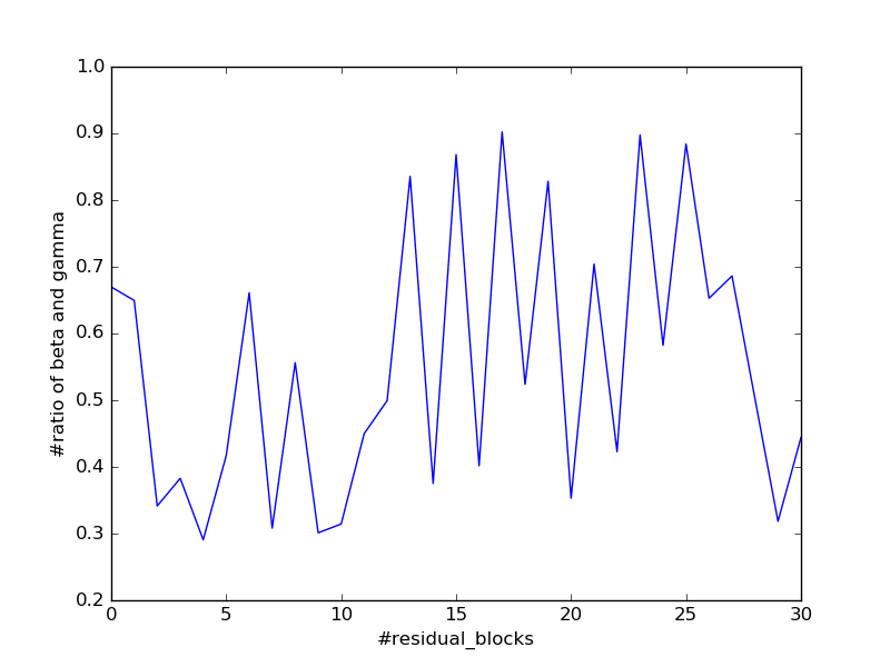
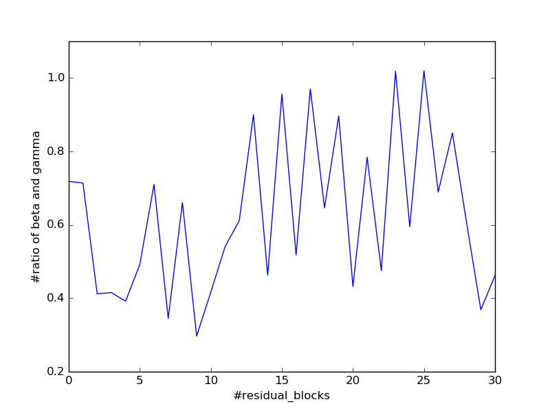
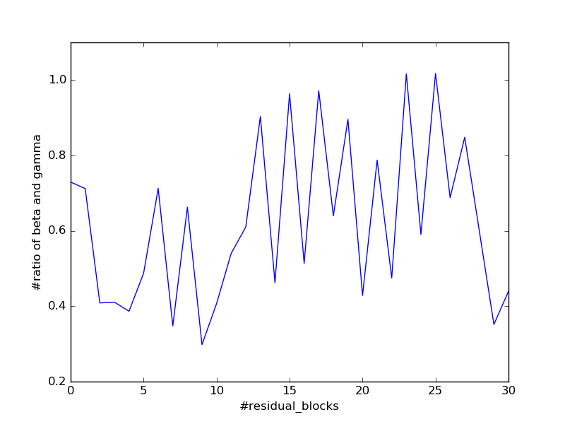
In this section, we show the experimental value of a = $\frac{\beta}{\gamma}$ during the training of residual networks containing 15 residual units. The mean of a (absolute value) at each layer stays reasonably small, atmost 1.0 in our case. This supports our theory that the constant term present in the upper and lower bounds of equation 14 are reasonably small constants so that our theory holds true.

Figure 13: The average of absolute value of $\frac{\beta}{\gamma}$, calculated for each layer, as a function of the residual block position at Epoch 25000 (left), Epoch 50000 (middle) and Epoch 75000 (right) in case of resnet-15.

Appendix G

In this section, we empirically show that our theory stays independent of the batch size used in stochastic gradient descent and also the initialization of weights in the network. Equation 14 is independent of the batch size used. Also, the initial variance of weights (within reasonable limits) doesn’t affect the behavior of gradient variance during training.

Figure 14: The variance of gradient as a function of residual block measured at step 25000, when batch size is 128 (left), 256 (middle) and 512 (right) respectively.

Figure 15: The variance of gradient as a function of residual block measured at step 25000, when the weights are initialized by 0.01(left) and 0.1(right) respectively.

References

- LeCun et al. (1989) Y. LeCun, B. Boser, J. S. Denker, D. Henderson, R. E. Howard, W. Hubbard, L. D. Jackel, Backpropagation applied to handwritten zip code recognition, Neural computation 1 (4) (1989) 541–551.
- Bengio et al. (2009) Y. Bengio, et al., Learning deep architectures for AI, Foundations and trends® in Machine Learning 2 (1) (2009) 1–127.
- Krizhevsky et al. (2012) A. Krizhevsky, I. Sutskever, G. E. Hinton, Imagenet classification with deep convolutional neural networks, in: Advances in neural information processing systems, 1097–1105, 2012.
- Simard et al. (1998) P. Simard, Y. LeCun, J. Denker, B. Victorri, Transformation invariance in pattern recognition—tangent distance and tangent propagation, Neural networks: tricks of the trade (1998) 549–550.
- Ioffe and Szegedy (2015) S. Ioffe, C. Szegedy, Batch normalization: Accelerating deep network training by reducing internal covariate shift, in: International Conference on Machine Learning, 448–456, 2015.
- Glo and Bengio (2015) X. Glo, Y. Bengio, Understanding the difficulty of training deep feedforward neural networks-glorot10a. pdf .
- Saxe et al. (2013) A. M. Saxe, J. L. McClelland, S. Ganguli, Exact solutions to the nonlinear dynamics of learning in deep linear neural networks, arXiv preprint arXiv:1312.6120 .
- He et al. (2015) K. He, X. Zhang, S. Ren, J. Sun, Delving deep into rectifiers: Surpassing human-level performance on imagenet classification, in: Proceedings of the IEEE international conference on computer vision, 1026–1034, 2015.
- Srivastava et al. (2015) R. K. Srivastava, K. Greff, J. Schmidhuber, Highway networks, arXiv preprint arXiv:1505.00387 .
- He and Sun (2015) K. He, J. Sun, Convolutional neural networks at constrained time cost, in: Proceedings of the IEEE Conference on Computer Vision and Pattern Recognition, 5353–5360, 2015.
- He et al. (2016) K. He, X. Zhang, S. Ren, J. Sun, Deep residual learning for image recognition, in: Proceedings of the IEEE conference on computer vision and pattern recognition, 770–778, 2016.
- Gers et al. (1999) F. A. Gers, J. Schmidhuber, F. Cummins, Learning to forget: Continual prediction with LSTM .
- Bengio et al. (1994) Y. Bengio, P. Simard, P. Frasconi, Learning long-term dependencies with gradient descent is difficult, IEEE transactions on neural networks 5 (2) (1994) 157–166.
- Greff et al. (2016) K. Greff, R. K. Srivastava, J. Schmidhuber, Highway and Residual Networks learn Unrolled Iterative Estimation, CoRR abs/1612.07771, URL http://arxiv.org/abs/1612.07771.
- Kuo and Chen (2017) C.-C. J. Kuo, Y. Chen, On Data-drive Saak Transform, arXiv preprint arXiv:1710.04176 .