Measuring the Stability of EHR- and
EKG-based Predictive Models
Abstract
Databases of electronic health records (EHRs) are increasingly used to inform clinical decisions. Machine learning methods can find patterns in EHRs that are predictive of future adverse outcomes. However, statistical models may be built upon patterns of health-seeking behavior that vary across patient subpopulations, leading to poor predictive performance when training on one patient population and predicting on another. This note proposes two tests to better measure and understand model generalization. We use these tests to compare models derived from two data sources: (i) historical medical records, and (ii) electrocardiogram (EKG) waveforms. In a predictive task, we show that EKG-based models can be more stable than EHR-based models across different patient populations.
1 Introduction
Patient history-based risk scores can inform physician decision-making and alter the course of treatment. The Framingham risk score for long-term coronary heart disease is one such an example [1]. In the past decade, large volumes of observational health care data — administrative claims, digitized physician notes, and laboratory test values among others — are now commonly used to build predictive models for a range of clinical purposes, including tracking disease progression [2], predicting near-term ICU interventions [3] or the onset of sepsis [4], and are incorporated into standardized prediction frameworks [5].
Patterns in observational health data, by construction, reflect health-seeking behavior in the population served. Consequently, predictive accuracy of statistical models can vary significantly if the underlying patterns of patient behavior vary in smaller groups within the population [6]. Further, under-served populations will, by definition, have less historical data on which to base predictive algorithms. Waveform and image data, such as electrocardiograms (EKGs) and echocardiograms, are a complementary source of information that can be used to build models of patient risk. EKGs, for instance, measure a patient’s cardiac function, which may be predictive of future disease. Patterns in a patient’s EKG (which directly measures cardiac activity) that are predictive of heart failure may be more portable than patterns in patient medical records across patient populations.
In this note, we study the generalization performance of predictive algorithms trained on one population and tested on another. We propose two statistics for measuring feature portability. As a case study, we construct models that predict the outcome of common lab test used to confirm heart attack — troponin levels — using (i) past diagnoses and medications and (ii) electrocardiogram waveform data. We show that EKG-based predictors are more stable across two sub-populations of patients — those that use the health care system with high frequency and those that use the system with lower frequency. For each prediction algorithm (e.g. data-source and training population), we examine the sources of distribution shift that can lead to poor generalization. We conclude with a discussion of future research directions.
2 Prediction and Conditional Stability
Our goal is to construct an accurate predictive model for some outcome (e.g. an adverse cardiac event) given some set of patient-specific data (e.g. historical medical records or raw EKG waveforms). We observe a set of these data drawn from a population distribution
| population distribution | (1) | ||||
| -distributed dataset of size . | (2) |
We use these data to train a model that predicts the conditional probability of given
| (3) |
where the model approximates the conditional distribution. For example, if are medical record features, may be a logistic regression model fit with maximum likelihood. If are EKG waveforms, may be a convolutional neural network.
Model Portability
How well does perform on another distribution, ? For example, the may be another hospital, health care system, or patient sub-population. For a specific model (e.g. logistic regression with EHR data) and a different sub-population , we can measure cross-generalization with the area under the ROC curve
| (4) |
where an entry denotes a model trained on population and tested on population . The diagonal entries measure the standard notion of generalization with no distribution shift — predictive performance on held out data from the same distribution. The off-diagonal entries measure performance under a new test distribution, a problem addressed by domain adaption techniques [7]. When generalization performance for population and population are different, a natural question is what is driving that gap? What features are portable?
Distribution shift
Why do predictive features fail to generalize? Consider a predictive model trained on data from population , which we denote with shorthand . The model is just a function of covariates . When is drawn from , and have a joint distribution, induced by . When is drawn from a different population , and have a different joint distribution, induced by . For shorthand, define . The conditional distributions induced by , , and can tell us what is “stable” and “unstable”
-
•
vs. : covariate stability
-
•
vs. : predictive stability
If covariates are conditionally unstable, this suggests different patterns of health-seeking behavior (or physiological differences) can be driving the generalization gap. If outcomes are conditionally unstable, this suggests that similar patterns in do not suggest the same way in population and population — there is something special about the prediction function tuned to population that does not apply to population .
We summarize covariate stability by estimating the distance between conditional distributions
| covariate stability | (5) |
where is the Kolmogorov-Smirnov distance between the two distributions — we use a two-sample estimator on held out data for this distance [8]. Intuitively, this will be low when covariates from the same class have the same distribution.
We summarize predictive stability with the difference in conditional expectation of given
| (6) |
This defines a function of — for each value of the conditional distribution of outcome may be similar or different between and . We visualize an estimate of this whole function, and compute a one dimensional summary (by averaging over an equal mixture of the and distributions).111The notation , and can appear confusing — there are really three distributions to keep in mind: the distribution of the model training set (), and the two distributions being compared (in our examples again and .)
3 Experiments
We build models that predict the outcome of a troponin lab test in a cohort of emergency department patients. A troponin test measures the troponin T or I protein levels, which are released when heart muscle is damaged during a heart attack. Troponin lab tests are used to determine if a patient is currently or about to suffer a heart attack. Based on the guidelines in [9], we define high to be a value of .04 ng/mL or greater. We label a patient “positive” () if they have received a troponin result greater than or equal to .04 ng/mL within the seven days following their emergency department admission. A patient is labeled “negative” () if they received a troponin result less than .04 ng/mL within the same time period. An algorithm that reliably predicts troponin outcome in the near term can be useful for assessing a patient’s risk of heart attack.
We study the stability of predictive models derived from two distinct sources of covariate () data:
-
•
ehr: all diagnoses and medications administered over the past year, derived from ICD-9 codes collected by a network of hospitals. We represent a patient’s one-year history with a sparse binary vector of 2,372 diagnoses and medications — a 1 indicates that the diagnosis/medication was present in the past year. We fit predictive models using ehr data with XGBoost [10], a gradient boosted decision tree algorithm, tuning tree depth using a validation set.
-
•
ekg: raw electrocardiogram waveforms from an EKG administered at the beginning of the emergency department visit. For the ekg data, we use the convolutional residual network described in [11] on the three “long leads” (II, V1, V5). We use stochastic gradient descent, keeping the model with the best predictive performance on a validation set.
Following the notation above, we study ehr- and ekg-based predictors over two populations:
-
•
high-use patients: patients with more than 8 visits to any department within the network of hospitals in the year before the emergency department encounter.
-
•
low-use patients: patients with 8 or fewer such visits in the same time frame.
Summary statistics of each population are presented in Table 1. We compare models derived from four combinations: trained on using features .
| trop | age | frac. female | |||||
| frac. pos | # pos | # obs | mean | std | mean | ||
| healthcare use | split | ||||||
| low | train | 0.119 | 832 | 7000 | 58.4 | 18.4 | 0.459 |
| val | 0.116 | 116 | 1000 | 58.4 | 18.2 | 0.447 | |
| test | 0.120 | 276 | 2298 | 58.2 | 18.4 | 0.438 | |
| high | train | 0.177 | 1236 | 7000 | 63.9 | 15.3 | 0.583 |
| val | 0.217 | 217 | 1000 | 62.2 | 17.1 | 0.533 | |
| test | 0.210 | 941 | 4491 | 63.5 | 15.5 | 0.555 | |
Generalization
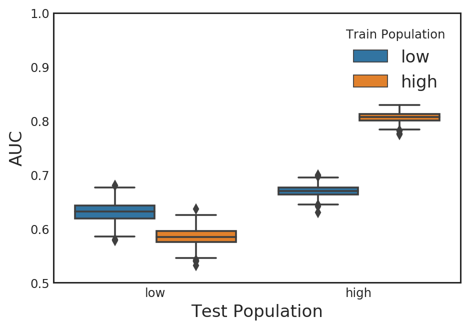
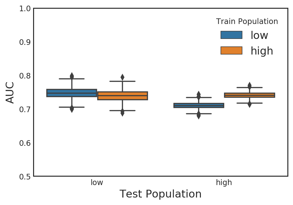
We present the within-distribution generalization performance (e.g. ) and the between-distribution performance (e.g. ) in Figure 1. The ehr model trained on the low-use () population generalizes slightly better on new patients from than the ehr model trained on the high-use () population. The ehr model trained on (high-use) generalizes significantly better on patients from than the model trained on patients from , as summarized in Figure 2(a). On the other hand, we see that models trained on ekg data from either or have similar predictive performance on both the and distributions, as seen in Figure 2(b).
Covariate stability
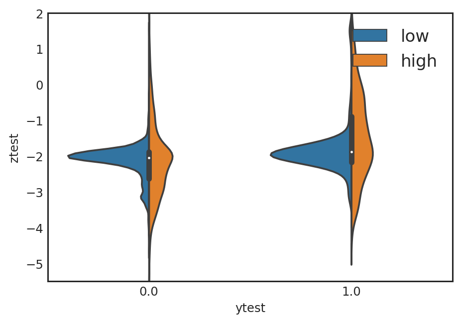
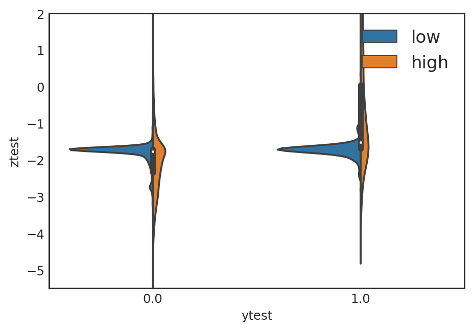
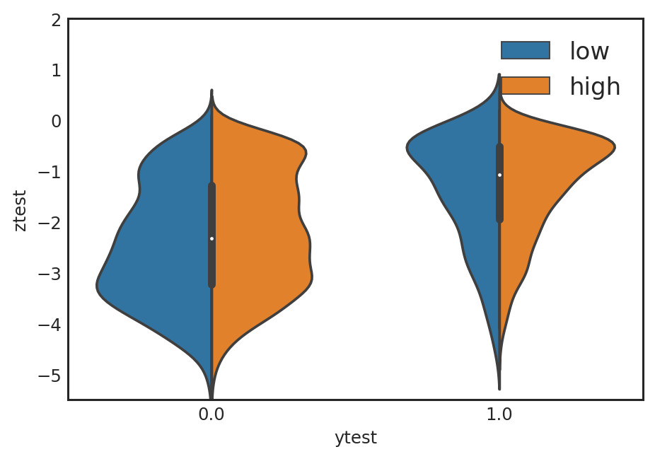
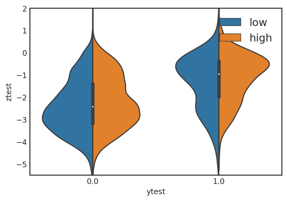
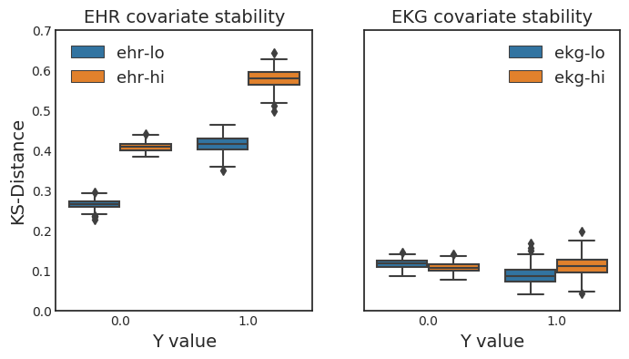
Figure 3 shows the covariate stability statistics for the two sets of models, trained on the two populations. We can see that the covariate distributions and are significantly closer when is based on ekg features than ehr features. This strongly suggests that behavioral characteristics between high- and low-use patients with the same outcome are driving a statistically significant difference in diagnosis and medication covariates . The ekg features, on the other hand, are significantly more stable between the high- and low-use patients. Intuitively, physiological measurements are not subject to the same biases that human behavior and decision-making introduce. The distributions of given and for both the ehr and ekg models are depicted in Appendix Figure 5.
Predictive stability
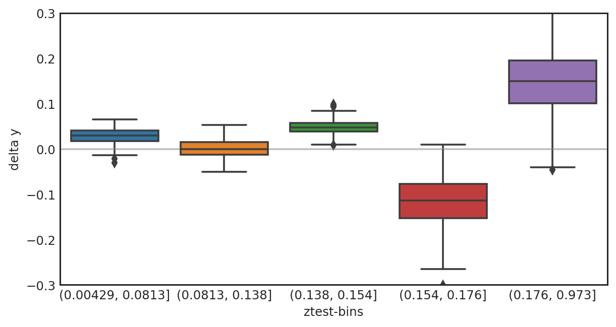
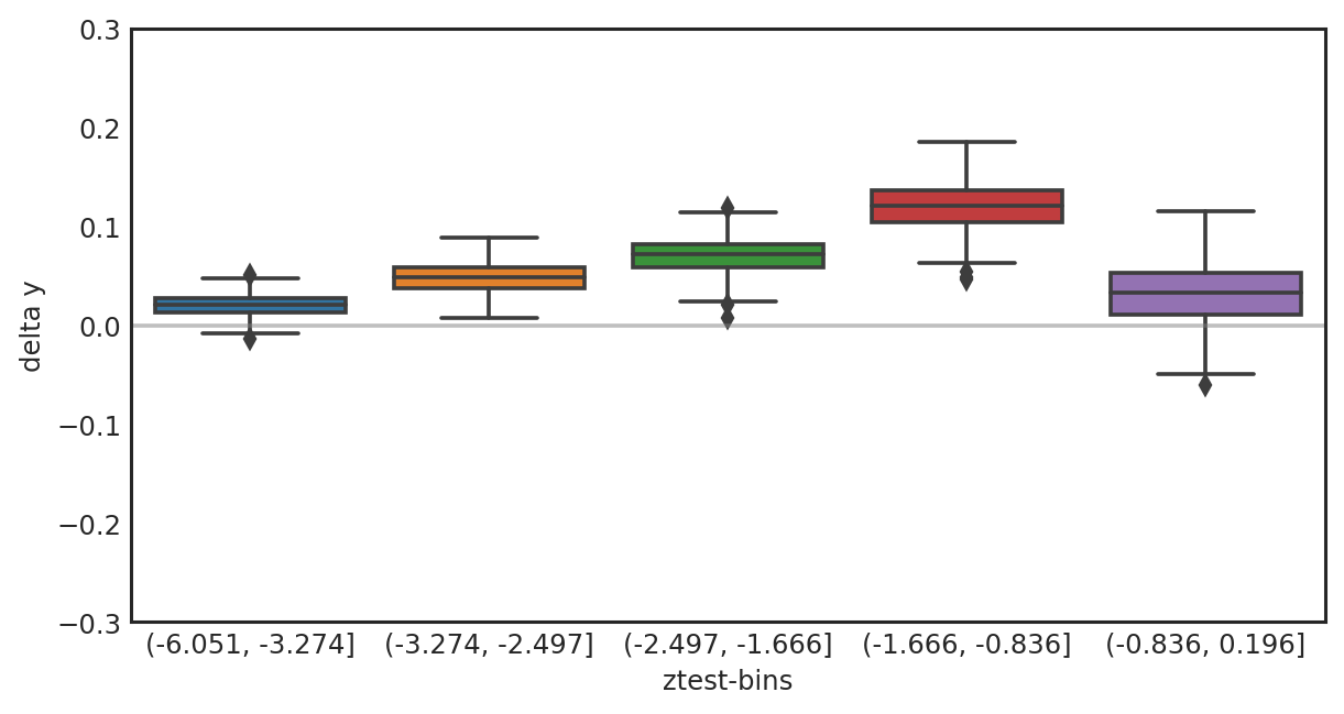
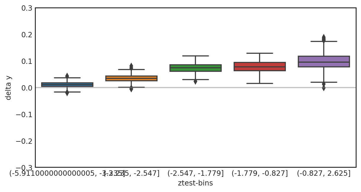
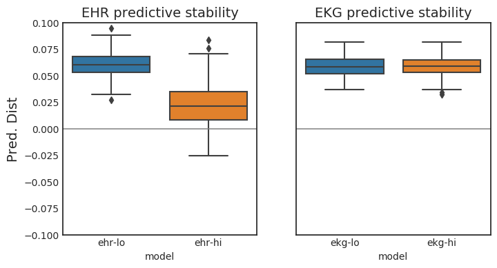
We present our one-dimensional predictive stability summary of Equation 6 in Figure 4, and depict full estimates in Figure . The average deviation between and are similar for the ekg and ehr models and small, though generally non-zero (on the order of .05 to .08). Both sets of models can make modest improvements, but this source of instability does not appear to be driving a large difference in generalization performance. More details are in Figure 6.
4 Discussion
We proposed two tests to better understand the portability of ehr and ekg features between patient populations. Our analysis suggests that EKG features can be stable across low- and high-use patients, whereas diagnoses and medications are not. We see multiple avenues of future work. Given the observed covariate instability, we hope to model patient health-seeking behavior which lead to statistical differences in ehr data. We also hope that models for patterns of missing data can be effectively combined with ekg data to construct a predictor that is both accurate and portable.
Additionally, it is presciently noted in [6] that a strategy for making predictors more equitable is to pay the cost of additional (and focused) data collection. Our analysis suggests a variant of this remedy — find sources of data that are more likely to generalize across populations. Physician notes, for example, are likely to be influenced by physician-specific biases, but are still may be more portable than billing records — a notion we hope to quantify and measure. EKGs and other physiological signals are not subject to the same patterns of presence and missingness in health record data, which is driven by unobserved human behavior and decision-making.
References
- Wilson et al. [1998] Peter WF Wilson, Ralph B D’Agostino, Daniel Levy, Albert M Belanger, Halit Silbershatz, and William B Kannel. Prediction of coronary heart disease using risk factor categories. Circulation, 97(18):1837–1847, 1998.
- Cruz and Wishart [2006] Joseph A Cruz and David S Wishart. Applications of machine learning in cancer prediction and prognosis. Cancer informatics, 2:117693510600200030, 2006.
- Ghassemi et al. [2017] Marzyeh Ghassemi, Mike Wu, Michael C Hughes, Peter Szolovits, and Finale Doshi-Velez. Predicting intervention onset in the icu with switching state space models. AMIA Summits on Translational Science Proceedings, 2017:82, 2017.
- Henry et al. [2015] Katharine E Henry, David N Hager, Peter J Pronovost, and Suchi Saria. A targeted real-time early warning score (trewscore) for septic shock. Science translational medicine, 7(299):299ra122–299ra122, 2015.
- [5] Jenna M Reps, Martijn J Schuemie, Marc A Suchard, Patrick B Ryan, and Peter R Rijnbeek. Design and implementation of a standardized framework to generate and evaluate patient-level prediction models using observational healthcare data. Journal of the American Medical Informatics Association.
- Chen et al. [2018] Irene Chen, Fredrik D Johansson, and David Sontag. Why is my classifier discriminatory? arXiv preprint arXiv:1805.12002, 2018.
- Ben-David et al. [2010] Shai Ben-David, John Blitzer, Koby Crammer, Alex Kulesza, Fernando Pereira, and Jennifer Wortman Vaughan. A theory of learning from different domains. Machine learning, 79(1-2):151–175, 2010.
- Stephens [1974] Michael A Stephens. Edf statistics for goodness of fit and some comparisons. Journal of the American statistical Association, 69(347):730–737, 1974.
- Newby et al. [2012] L Kristin Newby, Robert L Jesse, Joseph D Babb, Robert H Christenson, Thomas M De Fer, George A Diamond, Francis M Fesmire, Stephen A Geraci, Bernard J Gersh, Greg C Larsen, et al. Accf 2012 expert consensus document on practical clinical considerations in the interpretation of troponin elevations: a report of the american college of cardiology foundation task force on clinical expert consensus documents. Journal of the American College of Cardiology, 60(23):2427–2463, 2012.
- Chen and Guestrin [2016] Tianqi Chen and Carlos Guestrin. XGBoost: A scalable tree boosting system. In Proceedings of the 22nd ACM SIGKDD International Conference on Knowledge Discovery and Data Mining, KDD ’16, pages 785–794, New York, NY, USA, 2016. ACM. ISBN 978-1-4503-4232-2. doi: 10.1145/2939672.2939785. URL http://doi.acm.org/10.1145/2939672.2939785.
- Rajpurkar et al. [2017] Pranav Rajpurkar, Awni Y Hannun, Masoumeh Haghpanahi, Codie Bourn, and Andrew Y Ng. Cardiologist-level arrhythmia detection with convolutional neural networks. arXiv preprint arXiv:1707.01836, 2017.
Appendix A Additional Figures
