A Probabilistic Model of Cardiac
Physiology and Electrocardiograms
Abstract
An electrocardiogram (EKG) is a common, non-invasive test that measures the electrical activity of a patient’s heart. EKGs contain useful diagnostic information about patient health that may be absent from other electronic health record (EHR) data. As multi-dimensional waveforms, they could be modeled using generic machine learning tools, such as a linear factor model or a variational autoencoder. We take a different approach: we specify a model that directly represents the underlying electrophysiology of the heart and the EKG measurement process. We apply our model to two datasets, including a sample of emergency department EKG reports with missing data. We show that our model can more accurately reconstruct missing data (measured by test reconstruction error) than a standard baseline when there is significant missing data. More broadly, this physiological representation of heart function may be useful in a variety of settings, including prediction, causal analysis, and discovery.
1 Introduction
Heart disease annually claims the lives of over 600,000 people in the United States and over 17 million people worldwide [1, 2]. Early detection of cardiovascular disease is critical, and accurate characterization of patient risk can improve care. Consequently, a commonly used diagnostic tool is the electrocardiogram (EKG), which uses electrodes placed on the patient’s body to measure the heart’s electrical activity. EKGs are widely administered to diagnose a variety of cardiac abnormalities, including ischemia, heart attack, and arrhythmias. EKGs (and other waveform and image data) likely carry additional information about the overall health of a patient, beyond what is already in electronic health records (e.g. past diagnoses, medications, and lab tests). As we begin to use EHR data to inform health care decisions, EKG features can be used alongside patient EHR data to construct more accurate predictors, similar to unstructured physician notes [3] or the dynamics of ICU vital signs [4].
However, unlike discrete records, the EKG is a high-dimensional, dynamic object that is difficult to summarize. While an EKG could be summarized with standard ML tools, a generic approach would ignore the underlying physiology that drives EKG observations: the waveforms are a measurement of an electrical signal originating in the heart and propagating through the body.
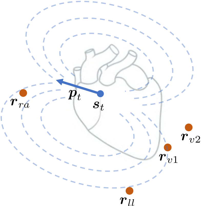
In this work, we pursue a physiological representation of an EKG by modeling the location, orientation, and strength of the electric potential induced by cardiac activity. Such a model has many benefits. First, because our model represents physical electrode locations, our approach can flexibly and coherently incorporate data from systems with more (or fewer) electrodes than standard 12-lead EKGs, including higher-dimensional (e.g.256-electrode body surface EKGs [5]) and lower-dimensional (e.g. 5-electrode Holter monitors) electrocardiographic signals. Second, we show that our model is robust to large amounts of missing observations. Finally, it produces a physically interpretable representation of the EKG that can be used in a variety of applications, such as prediction or causal analysis — for example, measuring the effect of a therapy on some aspect of cardiac function.
We evaluate our model with a lead reconstruction task — given an EKG where data from some leads are missing, how accurately can we reconstruct the held out data? We find that our model can more accurately reconstruct missing EKG leads than non-physical factor models when we have a lot of missing data (which is common in our clinical emergency department setting). We conclude with a discussion of statistical inference challenges and model extensions.
2 Data Description and Model
EKG Background
An EKG lead measures the electric potential difference between two (or more) electrodes. An electrode is a conductive pad placed on a part of the body (e.g. left leg or chest) that measures instantaneous electric potential. A lead records the difference between a pair (or a specific combination) of electrode readings (typically in millivolts); cardiologists visually inspect the lead outputs for abnormalities. The standard twelve leads are commonly referred to as .111There are typically nine electrodes used to produce a twelve lead EKG — see Appendix A. An EKG tracing of length consists of -dimensional observations at time steps,
| (1) |
We model lead EKG observations by describing the physical location, orientation, and strength of the electric potential induced by cardiac activity. We introduce model components that (i) describe the underlying state of electrical activity; (ii) map latent electrical activity to electrode potential values; and (iii) map electrode values to lead observations. To address point (i) we model electrical activity with a single moving dipole, following [6]. We address point (ii) by modeling the 3-d location of electrodes and using a simplified torso conductance model. Point (iii) is straightforward and can be modeled by a fixed linear map — we describe this step in detail in Appendix A.
Moving Dipole Generative Model
Each observation is generated by the electric potential induced by a single latent dipole with state , where is the spatial location of the dipole and is its moment. A dipole is an idealized point whose location and moment induce a spatial electrostatic potential that is measured by each electrode. At time , the latent dipole induces a potential at each of the electrodes that are spatially located at points where and . Assuming a uniform conductance torso model, a single dipole with state will have a potential measured at electrode , located at , given by
| (2) |
where is the (constant) electrical conductivity of the torso [6] (which we set to , following [7]). To get from electrode to lead, there is a fixed linear function which produces the twelve standard leads, namely , where and is detailed in Appendix A.
Priors
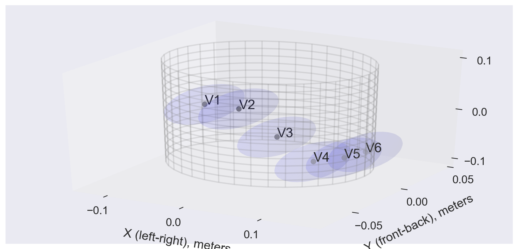
To complete the model, we specify a prior distribution over the latent dipole state, and , and the location of each electrode . We put zero-centered spherical Gaussian priors over and and weakly informative priors over electrode locations, , described in Appendix B.1. The data generating process is
| (3) | |||||
| (4) | |||||
| (5) |
In this current iteration we ignore temporal correlation in and , leaving this for future work.
Inference
The above generative model will admit tractable (though approximate) variational inference [8]. As a first step, however, we use MAP inference to show the utility of this modeling approach, solving the optimization problem
| (6) | ||||
| (7) |
To solve this optimization problem, we use L-BFGS [9] with gradients computed by automatic differentiation [10]. See Section D for further discussion of inference.
3 Experiments
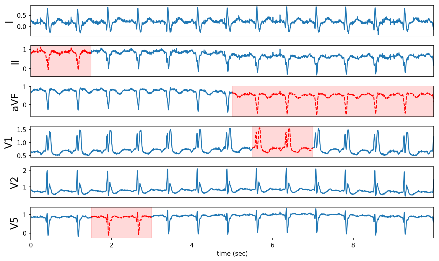
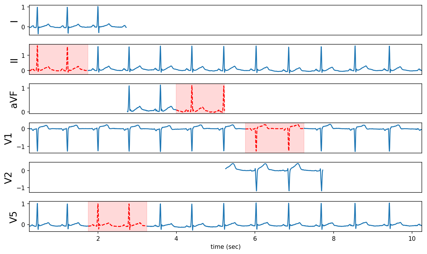
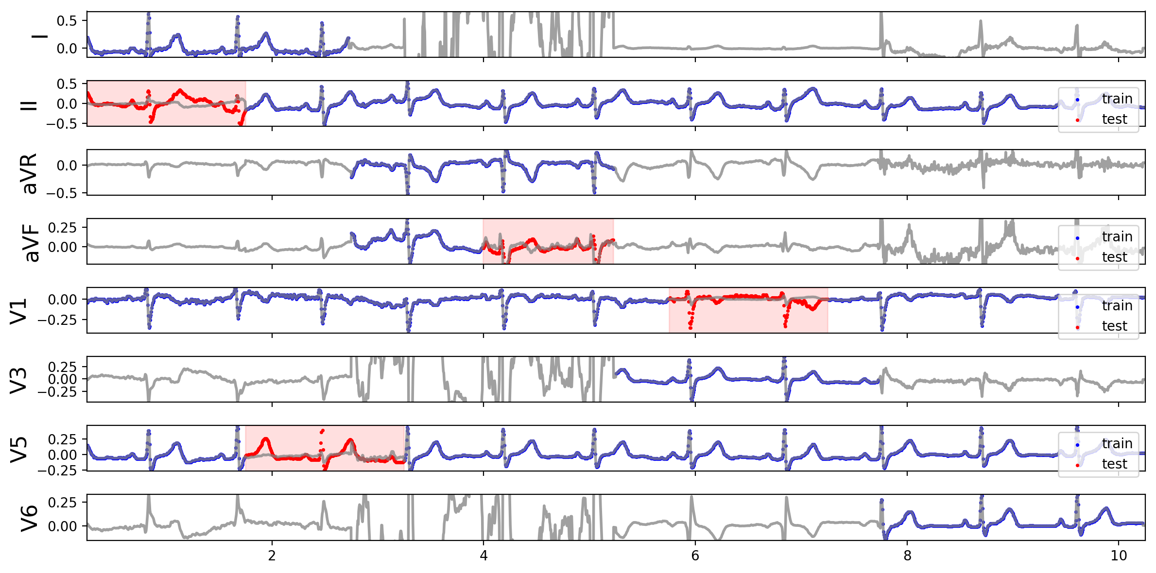
We assess model performance by measuring held-out lead reconstruction error. For each EKG, we hold out portions of the waveform during training (depicted in Figure 2). We then use the model to impute the held-out values and compute the root mean squared error (RMSE). A model that better captures the underlying phenomenon will more accurately impute missing lead values.
We apply our model to a small sample of 10-second EKG segments from two datasets:
- •
-
•
ed: a subset of 997 EKG recordings from emergency department patients from a large metropolitan hospital, each exhibiting “normal sinus rhythm.” These EKGs are derived from a traditional report that saves the full time series for leads II, V1, and V5, and short (approximately 2.5 second) segments of the other 9 leads. This missingness can frustrate analysis of the full EKG object, which we address with both our model and baseline approaches. Figure 2(b) shows a typical ed record.
Baseline linear factor model
We compare the latent dipole model to probabilistic PCA (with and latent dimensions), which describes lead observations as
| (8) |
Here are the latent factors, and is the -dimensional latent state that describes observation (analogous to our dipole location and moment). We use an implementation of PCA designed to handle missing entries [12].
Empirical Results
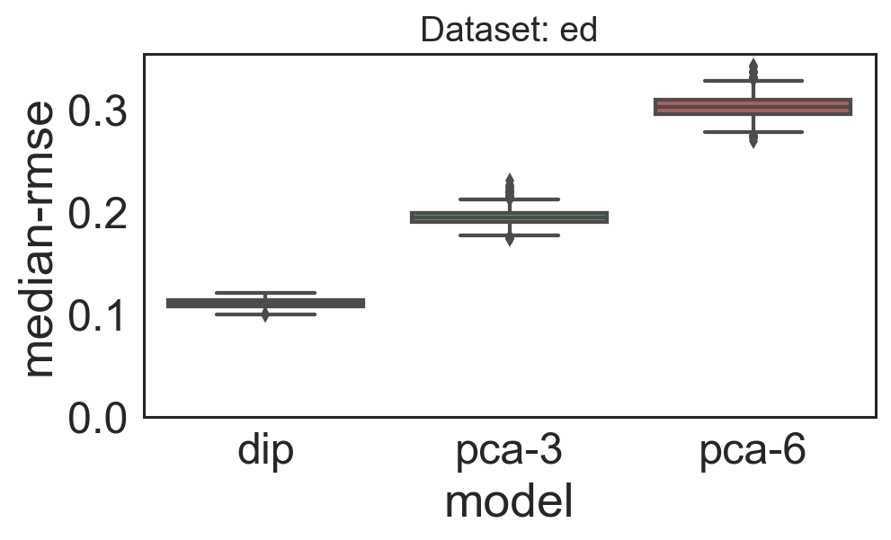
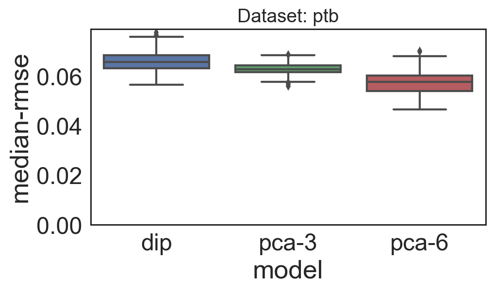
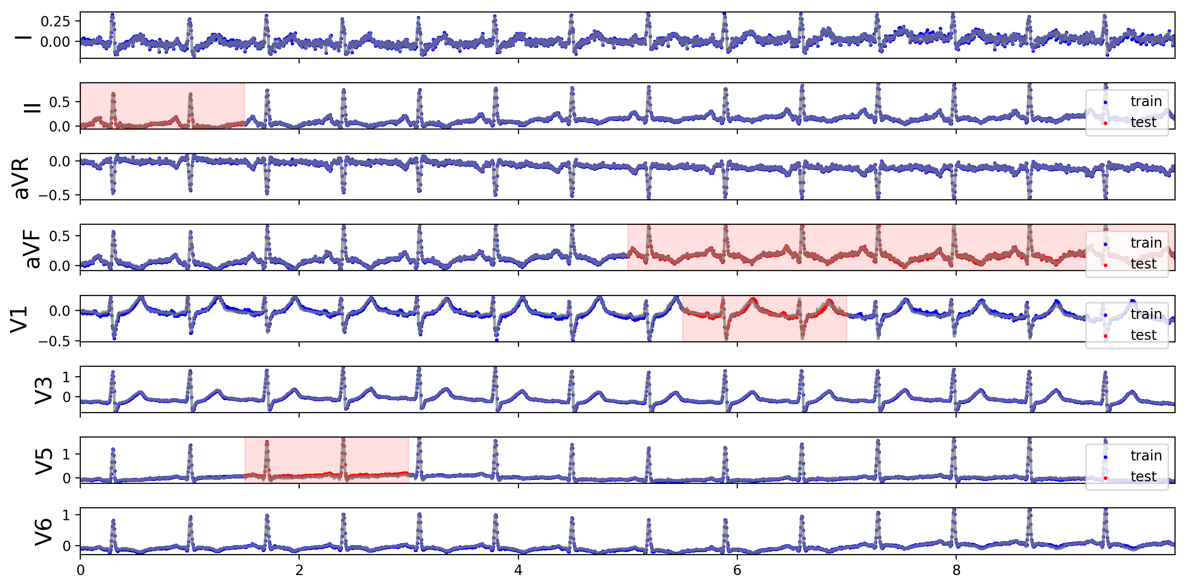
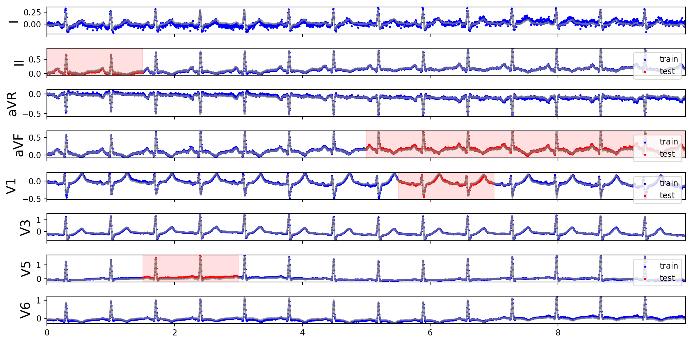
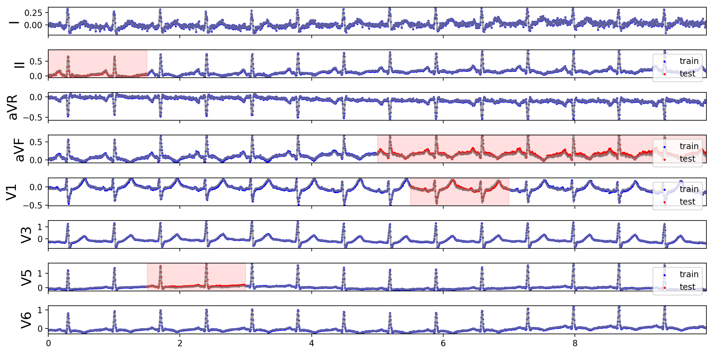
For each dataset, we fit the dipole model and two PCA models ( and ) to each EKG. We compare the median RMSE over all patients in each dataset. Figure 3 depicts the median RMSE for each model for the ed and ptb. We observe that the dipole model more reliably reconstructs out of sample lead observations in the ed setting, where the short leads are missing most entries (see Figure 2). We observe similar performance for all three models in the ptb dataset. The dipole model is constrained to produce a spatially consistent reconstruction of EKG leads, which may help in the absence of many lead observations.
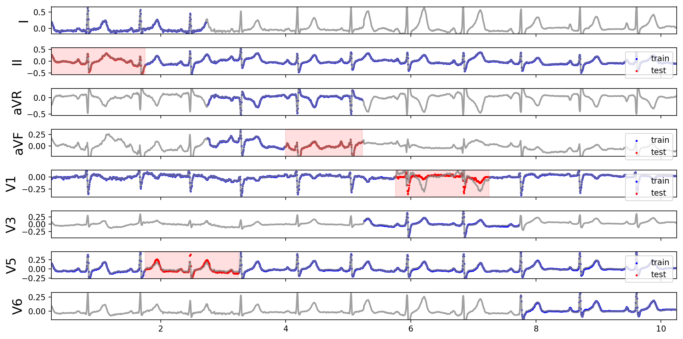
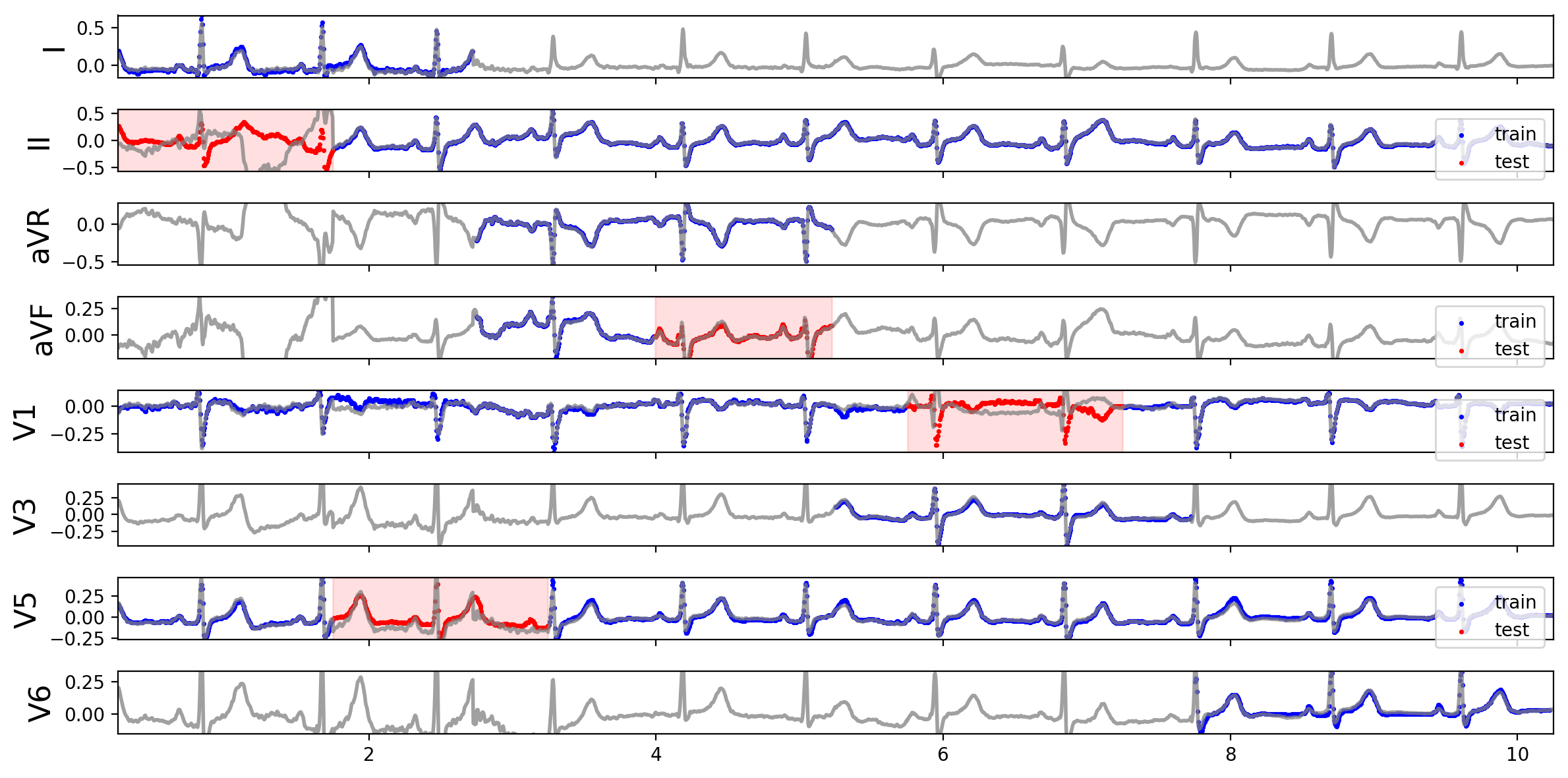
We produce a full imputation of an ed EKG in Figure 5, which shows that the dipole model can have more stable imputations. To contrast this, the ptb EKG imputation in Figure 6 shows that both models have an easier time reconstructing out of sample leads when most of the tracing is present. Figure 4(a) shows the dipole model reconstruction on an ed EKG. Figure 4(b) compares the residuals for the dipole model and two PCA models on the same EKG. We see that the dipole model accurately reconstructs leads II and aVF (almost no structure in the residual), but has a difficult time with the precordial leads V1 and V5, which may be due to inaccurate reconstruction of electrode location. The PCA models have structured residuals for all leads around regions of high voltage.
4 Discussion
We developed a model of EKG observations with a physiological inductive bias. We compared our model to non-physical latent factor models, showing its potential to more accurately characterize patient physiology. There are many directions of future work. We will model temporal dynamics in the latent variables , incorporating local temporal smoothness and quasi-periodicity into the prior. Such dynamics may better characterize arrhythmias or other abnormalities not present in normal sinus rhythm EKGs. The non-conjugacy of the dipole-electrode model complicates inference; a focus will be on efficient approximate inference methods for this model, following [13] and [14]. We also aim to use model output in downstream statistical analyses — exploring the structure of patients with adverse cardiac events, building risk predictors alongside historical patient medical record that can aid physician decision-making, and measuring the causal effect of therapies on aspects of cardiac function.
References
- for Disease Control [2017] Center for Disease Control. Heart disease facts. https://www.cdc.gov/heartdisease/facts.htm, 2017.
- Organization [2017] World Health Organization. Cardiovascular disease. http://www.who.int/cardiovascular_diseases/en/, 2017.
- Rumshisky et al. [2016] A Rumshisky, M Ghassemi, T Naumann, P Szolovits, VM Castro, TH McCoy, and RH Perlis. Predicting early psychiatric readmission with natural language processing of narrative discharge summaries. Translational psychiatry, 6(10):e921, 2016.
- Ghassemi et al. [2017] Marzyeh Ghassemi, Mike Wu, Michael C Hughes, Peter Szolovits, and Finale Doshi-Velez. Predicting intervention onset in the icu with switching state space models. AMIA Summits on Translational Science Proceedings, 2017:82, 2017.
- Cluitmans et al. [2015] MJM Cluitmans, RLM Peeters, RL Westra, and PGA Volders. Noninvasive reconstruction of cardiac electrical activity: update on current methods, applications and challenges. Netherlands Heart Journal, 23(6):301–311, 2015.
- Okamoto et al. [1982] Yoshiwo Okamoto, Yasuaki Teramachi, Toshimitsu MUSHA, Hiroshi Tsunakawa, and Ken-ichi Harumi. Moving multiple dipole model for cardiac activity. Japanese heart journal, 23(3):293–304, 1982.
- Sovilj et al. [2013] Siniša Sovilj, Ratko Magjarević, Nigel H Lovell, and Socrates Dokos. A simplified 3d model of whole heart electrical activity and 12-lead ecg generation. Computational and mathematical methods in medicine, 2013.
- Ranganath et al. [2014] Rajesh Ranganath, Sean Gerrish, and David Blei. Black box variational inference. In Artificial Intelligence and Statistics, pages 814–822, 2014.
- Liu and Nocedal [1989] Dong C Liu and Jorge Nocedal. On the limited memory bfgs method for large scale optimization. Mathematical programming, 45(1-3):503–528, 1989.
- Maclaurin et al. [2015] Dougal Maclaurin, David Duvenaud, and Ryan P Adams. Autograd: Effortless gradients in numpy. 2015.
- Goldberger et al. [2000] AL Goldberger, LA Amaral, L Glass, JM Hausdorff, PC Ivanov, RG Mark, JE Mietus, GB Moody, CK Peng, and HE Stanley. Physiobank, physiotoolkit, and physionet: components of a new research resource for complex physiologic signals. Circulation, 101(23):E215–20, 2000. URL https://physionet.org/physiobank/database/ptbdb/.
- Bailey [2012] Stephen Bailey. Principal component analysis with noisy and/or missing data. Publications of the Astronomical Society of the Pacific, 124(919):1015, 2012.
- Gao et al. [2016] Yuanjun Gao, Evan W Archer, Liam Paninski, and John P Cunningham. Linear dynamical neural population models through nonlinear embeddings. In Advances in neural information processing systems, pages 163–171, 2016.
- Johnson et al. [2016] Matthew Johnson, David K Duvenaud, Alex Wiltschko, Ryan P Adams, and Sandeep R Datta. Composing graphical models with neural networks for structured representations and fast inference. In Advances in neural information processing systems, pages 2946–2954, 2016.
- Geselowitz [1989] David B Geselowitz. On the theory of the electrocardiogram. Proceedings of the IEEE, 77(6):857–876, 1989.
Appendix A Electrode to Lead transformation
Electrocardiogram data are presented as leads, which are differences in potential values between electrode measurements (or averages of electrode measurements). This is a somewhat straightforward transformation that we will account for in the likelihood. The output potential difference for each lead are simple functions of the electrode readings:
We can express these relationships as a simple linear transformation of the electrode values into lead values
| (9) |
where the transformation matrix has a fixed block structure, where the blocks are defined
| (10) |
Appendix B Priors
B.1 Electrode location prior
Fitting data with the above appearance model will require inferring the electrode locations . We can use the general guidelines of where to attach electrodes to place a prior on their relative location.
We use a simple elliptical model of the thorax to set prior values on the location of V1 - V6. We set the chest width to be 25 centimeters and the major-minor axis ratio to be 2.75. The V1 - V6 locations are at even angular locations from 260 degrees to 360 degrees (all the way to the left side of the chest). Figure 1(b) depicts the prior (with 2 standard deviations for the precordial (chest) electrodes (v1 - v6).
The location of the right arm, left arm, and left leg electrodes will be given diffuse priors flanking the modeled torso depicted in Figure 1(b).
B.2 Conductance Parameter Priors
Average thoracic tissue impedance can be approximated as resistive with conductivity values around .2 S/m [15].
Appendix C Additional Model Fit
Figure 4 depicts held-out data, showing the reconstruction performance of the dipole model in leads V1, V5, II and aVF. Figure 4(b) also depicts the residuals for the dipole model and both PCA models. Figure 5 displays the full missing data imputation for an emergency department patient. Similarly, Figure 6 shows the missing data imputation for the ptb example, which has no missing data.


Appendix D Inference
We currently fit the model with MAP inference over both the latent and global parameters. This joint maximization, however, may lead to overfitting — we would prefer to maximize the following marginal likelihood objective
| (11) | ||||
| (12) |
As an example, this is the objective that PCA essentially fits — the local weights are integrated out (in the E-step) and the global factors are optimized (in the M-step).
Our dipole is challenging, however, because the latent factors and global variables enter into the likelihood term, with a complex function, given by Equation 5.
The posterior distribution over given the observations and electrode locations does not admit a closed form
| (13) | ||||
| (14) | ||||
| (15) |
where we define to be the -length electrode observations
| (16) |
recalling that the latent state is divided into a location and moment component. Because is nonlinear in , the posterior distribution over becomes intractable. We do note that is linear in when you fix , , and . If we place a Gaussian prior over , this conditional posterior should be tractable. We plan to use this tractable conditional structure in future work to scale inference in this model.