Stochastic Galerkin method for cloud simulation

Abstract.

We develop a stochastic Galerkin method for a coupled Navier-Stokes-cloud system that models dynamics of warm clouds. Our goal is to explicitly describe the evolution of uncertainties that arise due to unknown input data, such as model parameters and initial or boundary conditions. The developed stochastic Galerkin method combines the space-time approximation obtained by a suitable finite volume method with a spectral-type approximation based on the generalized polynomial chaos expansion in the stochastic space. The resulting numerical scheme yields a second-order accurate approximation in both space and time and exponential convergence in the stochastic space. Our numerical results demonstrate the reliability and robustness of the stochastic Galerkin method. We also use the proposed method to study the behavior of clouds in certain perturbed scenarios, for examples, the ones leading to changes in macroscopic cloud pattern as a shift from hexagonal to rectangular structures.

1. Introduction

Clouds constitute one of the most important component in the Earth-atmosphere system. They influence the hydrological cycle and by interacting with radiation they control the energy budget of the system. However, clouds are one of the most uncertain components, which, unlike the atmospheric flows, cannot be modeled using first principles of physics.

Clouds are composed by myriads of water particles in different phases (liquid and solid), and thus they need to be described by a large ensemble in a statistical sense. A common way of obtaining such an ensemble is by using a mass or size distribution, which would lead to a Boltzmann-type evolution equation. Although there are some approaches available in literature to formulate cloud models in such a way [4, 18, 17], a complete and consistent description is missing. Since measurements of size distributions of cloud particles are difficult, we are often restricted to averaged quantities such as, for example, mass of water per dry air (mass concentrations). Therefore, models are often formulated in terms of so-called bulk quantities, that is, mass and number concentrations of the respective water species. Many cloud processes are necessary to describe the time evolution of the cloud as a statistical ensemble, that is, particle formation or annihilation, growth/evaporation of particles, collision processes, and sedimentation due to gravity. For each of the processes, we have to formulate a representative mathematical term in the sense of a rate equation. Although for some processes the physical mechanisms are quite understood, the formulation of the process rates usually contain uncertain parameters, thus cloud models come with inherent uncertainty. On the other hand, the initial conditions for atmospheric flows and the embedded clouds are also not perfectly constrained, leading to uncertainties in the environmental conditions. It is well-known from former studies that uncertainties in cloud processes and in environmental conditions can lead to drastic changes in simulations, thus these uncertainties influence predictability of moist atmospheric flows, clouds and precipitation in a crucial way; for instance, the distribution of latent heat is changed, which in turn can influence frontogenesis [15] or convection [14, 24].

For investigations of the impact of these uncertain cloud model parameters as well as the impact of variations in environmental conditions on atmospheric flows, sensitivity studies are usually carried out. Since one or more parameters are (randomly) varied, the Monte Carlo approach can be used. This, however, requires a large ensemble of simulations to be conducted, which makes Monte Carlo methods computationally expensive and requires a very fine sampling of the parameter space and possible environmental conditions. In most practical studies, a much smaller set of ensembles (with about $10-100$ samples only) is used.

In order to improve both the efficiency and accuracy of a numerical method, we choose a different way of representing random variations by using spectral expansions in the stochastic space. This approach enables us to investigate the impact of variations in cloud model parameters and initial conditions on the evolution of moist flows with embedded clouds.

We consider a mathematical model of cloud physics that consists of the Navier-Stokes equations coupled with the cloud evolution equations for the water vapor, cloud water and rain. In this model developed in [22, 34] and presented in Section 2, the Navier-Stokes equations describe weakly compressible flows with viscous and heat conductivity effects, while microscale cloud physics is modeled by the system of advection-diffusion-reaction equations.

Meteorological applications typically inherit several sources of uncertainties, such as model parameters, initial and boundary conditions. Consequently, purely deterministic models are insufficient in such situations and more sophisticated methods need to be applied to analyze the influence of uncertainties on numerical solutions. In this paper, we study a stochastic version of the coupled Navier-Stokes-cloud model in order to account for uncertainties in input quantities. Our main goal is to design an efficient numerical method for quantifying uncertainties in solutions of the studied system. In recent years, a wide variety of uncertainty quantification methods has been proposed and investigated in the context of physical and engineering applications. These methods include stochastic Galerkin methods based on generalized polynomial chaos (gPC) [46, 33, 40, 41, 10], stochastic collocation methods [23, 44, 45], and multilevel Monte Carlo methods [37, 29, 28]. Each of these groups of methods has its own pros and cons. While results obtained by the Monte Carlo simulations are generally good, the approach is not very efficient due to a large number of realizations required. Stochastic collocation methods are typically more efficient than the Monte Carlo ones, since they only require solving the underlying deterministic system at the certain quadrature nodes in the stochastic space. These data are then used to reconstruct the gPC expansion using an appropriate set of orthogonal polynomials. The Monte Carlo as well as the stochastic collocation method fall into a class of the non-intrusive methods. Stochastic Galerkin methods offer an alternative approach for computing the gPC expansion. In general, they are more rigorous and efficient than the Monte Carlo and collocation ones; see, e.g., [12]. The stochastic Galerkin method is an intrusive method since it requires changes in the underlying code. In fact, one needs to solve a system of PDEs for the gPC expansion coefficients.

We develop a new stochastic Galerkin method for the coupled Navier-Stokes-cloud system. As it has already been mentioned above, the largest source of uncertainties is cloud physics. Therefore, we restrict our consideration to the case in which the uncertainties are only in the cloud physics representation; extension to full stochastic Navier-Stokes-cloud model is left to future studies. Thus, we need to solve the deterministic Navier-Stokes equations coupled with the PDE system for the gPC expansion coefficients for the cloud variables. Our numerical method is an extension of the approach proposed in [22] for the purely deterministic version of the coupled Navier-Stokes-cloud system. This method is based on the operator splitting approach, in which the system is split into the macroscopic Navier-Stokes equations and microscopic cloud model with random inputs. The Navier-Stokes equations are then solved by an implicit-explicit (IMEX) finite-volume method, while for the cloud equations we develop a stochastic Galerkin method based on the gPC. The resulting gPC coefficient system is numerically solved by a finite-volume method combined with an explicit Runge-Kutta method with an enlarged stability region [27].

The paper is organized as follows. We start in Section 2 with the description of the deterministic Navier-Stokes-cloud model. The numerical method for the deterministic model is presented in Sections 3. In Sections 4, we report on numerical experiments for well-known meteorological benchmarks—rising warm bubble and Rayleigh-Bénard convection—for the deterministic model. We then continue in Section 5 with the presentation of the stochastic model, which is followed by the description of the numerical method (Section 6) and presentation of the numerical experiments (Section 7) for the stochastic model. Our numerical results clearly demonstrate that the proposed stochastic Galerkin method is capable of quantifying the uncertainties of complex atmospheric flows.

2. Deterministic mathematical model

We study a mathematical model of cloud dynamics, which is based on the compressible nonhydrostatic Navier-Stokes equations for moist atmosphere (that is, mixture of ideal gases dry air and water vapor),

$$\rho_{t}+\nabla\cdot\left(\rho\bm{u}\right) =0,$$

$$(\rho\bm{u})_{t}+\nabla\cdot\left(\rho\bm{u}\otimes\bm{u}+p\,{\rm Id}-\mu_{m}\rho\left(\nabla\bm{u}+(\nabla\bm{u})^{\top}\right)\right) =-\rho g\bm{e_{3}},$$ (2.1)

$$(\rho\theta)_{t}+\nabla\cdot\left({\rho\theta}\bm{u}-\mu_{h}\rho\nabla\theta\right) =S_{\theta},$$

and evolution equations for cloud variables,

$$(\rho q_{v})_{t}+\nabla\cdot\left(\rho q_{v}\bm{u}-\mu_{q}\rho\nabla q_{v}\right) =\rho(-C+E),$$

$$(\rho q_{c})_{t}+\nabla\cdot\left(\rho q_{c}\bm{u}-\mu_{q}\rho\nabla q_{c}\right) =\rho(C-A_{1}-A_{2}),$$ (2.2)

$$(\rho q_{r})_{t}+\nabla\cdot\left(-v_{q}\rho q_{r}\bm{e_{3}}+\rho q_{r}\bm{u}-\mu_{q}\rho\nabla q_{r}\right) =\rho(A_{1}+A_{2}-E).$$

Here, $\rho$ is the density, $\bm{u}=(u_{1},u_{2},u_{3})^{\top}$ is the velocity vector, $\theta$ is the moist potential temperature, $p$ is the pressure, $g$ is the acceleration due to gravity, $\mu_{m}$ is the dynamic viscosity, $\mu_{h}$ is the thermal conductivity, and $\mu_{q}$ is the cloud diffusivity. The cloud variables representing the mass concentration of water vapor, cloud droplets and rain drops, $q_{v}$, $q_{c}$, $q_{r}$, respectively, as well as the right-hand side (RHS) terms $E$, $C$, $A_{1}$, $A_{2}$ will be defined below. We denote by $t$ the time variable and by $\bm{x}$ the space vector; $\bm{x}=(x_{1},x_{2},x_{3})$ in the three-dimensional (3-D) and $\bm{x}=(x_{1},x_{3})$ in the two-dimensional (2-D) cases. Furthermore, $\bm{e_{3}}=(0,0,1)^{\top}$ and $\bm{e_{3}}=(0,1)^{\top}$ in the 3-D and 2-D cases, respectively. We set $\mu_{m}=10^{-3}$ and $\mu_{h}=10^{-2}=\mu_{q}$. Note that the systems (2) and (2) are coupled through the source term $S_{\theta}$, which represents the impact of phase changes and will be defined below, see (2.6). The temperature $T$ can be obtained from the moist adiabatic ideal gas equation

$$T=\frac{R}{R_{m}}\theta\left(\frac{p}{p_{0}}\right)^{\nicefrac{{R_{m}}}{{c_{p}}}},$$ (2.3)

where $p_{0}=10^{5}\,\mathrm{Pa}$ is the reference pressure at sea level. In addition to the usual definition of a potential temperature, we use $R_{m}=(1-q_{v}-q_{c}-q_{r})R+q_{v}R_{v}$ with the ideal gas constant of dry air $R=287.05\,\mathrm{\nicefrac{{J}}{{(kg\cdot K)}}}$, the gas constant of water vapor $R_{v}=461.51\,\mathrm{\nicefrac{{J}}{{(kg\cdot K)}}}$ and the specific heat capacity of dry air for constant pressure $c_{p}=1005\,\mathrm{\nicefrac{{J}}{{(kg\cdot K)}}}$. In order to close the system, we determine the pressure from the equation of state that includes moisture

$$p=p_{0}\left(\frac{R\rho\theta}{p_{0}}\right)^{\gamma_{m}}\quad\mbox{with}\quad\gamma_{m}=\frac{c_{p}}{c_{p}-R_{m}}.$$ (2.4)

We note that in the dry case $R_{m}$ reduces to $R$, $S_{\theta}=0$ and the moist ideal gas equation as well as the moist equation of state become their dry analogon.

In this paper, we restrict our investigations to clouds in the lower part of the troposphere, that is, to clouds consisting of liquid droplets exclusively. All of the processes involving ice particles are left for future research. For the representation of liquid clouds in our model we use the so-called single moment scheme, that is, equations for the bulk quantities of mass concentrations of different water phases. For the representation of the relevant cloud processes we adapt a recently developed cloud model [34]. Note that for bulk models, the process rates cannot be derived completely from first principles. Consequently, some uncertain parameters show up naturally. This underlies the need of a rigorous sensitivity study which is the goal of the present paper.

Generally, we follow the standard approach in cloud physics modeling for separating hydrometeors of different sizes, as firstly introduced in [16]. This relies on the observations that small droplets have a negligible falling velocity. In addition, measurements indicate two different modes of droplets in the size distribution, which can be associated to small cloud droplets and large rain drops [42]. Thus, we use the cloud variables $q_{c}$ and $q_{r}$ indicating mass concentration of (spatially stationary) cloud droplets and (falling) rain drops, respectively, and the water vapor concentration $q_{v}$, that is,

$$q_{\ell}=\frac{\mbox{mass of the respective phase}}{\mbox{mass of dry air}}\quad\mbox{for}\quad\ell\in\{v,c,r\}.$$

The rest of this section is devoted to a description of the different terms on the RHS of (2), which represents the following relevant cloud processes, see [34].

2.1. Single particle properties

• General properties of a single water particle

  As we exclusively investigate water clouds, we can assume a spherical shape of water particles. For small cloud droplets this is a very good approximation, while for large rain drops drag effects change their shape [38, 39]. However, for our investigations of ensembles of rain drops, the spherical shape approximation is appropriate. Thus, mass and radius of droplets are related by the usual equation

  $$m=\frac{4}{3}\pi\rho_{\ell}r^{3}\quad\iff\quad r=\left(\frac{3}{4\pi\rho_{\ell}}\right)^{\frac{1}{3}}m^{\frac{1}{3}}$$

  with the liquid water density $\rho_{\ell}=10^{3}\,\mathrm{kg\,m^{-3}}$. We make a general assumption that small cloud droplets are stationary, while large rain drops are accelerated by gravity. After balancing gravity by frictional forces, spherical rain drops fall with a terminal velocity, depending only on the drop mass and the density of air. According to [34], the terminal velocity for a droplet of mass $m$ is given by

  $$\hskip 28.45274ptv_{\tau}(m)=\alpha\,m^{\beta}\left(\frac{m_{\tau}}{m_{\tau}+m}\right)^{\beta}\left(\frac{\rho_{*}}{\rho}\right)^{\frac{1}{2}},\quad\alpha=190.3\,\mathrm{m\,s^{-1}\,kg^{-\beta}},\quad\beta=\frac{4}{15},\quad m_{\tau}=1.21\cdot 10^{-5}\mathrm{kg},$$

  with the reference density $\rho_{*}=1.255\,\mathrm{kg\,m^{-3}}$ at $T_{*}=288\,\mathrm{K}$ and $p_{*}=101\,325\,\mathrm{Pa}$. For masses $m\ll m_{\tau}$, we can approximate the terminal velocity by $v_{\tau}=\alpha\,m^{\beta}\sqrt{\frac{\rho_{*}}{\rho}}$; this approximation will be used in the description of the process accretion (collection of cloud droplets by rain drops).

• Diffusion processes: Growth and evaporation

  Diffusion processes (transfer of water molecules to and from the liquid particle) can be described by the following growth equation:

  $$\frac{dm}{dt}=-4\pi rD_{v}G\rho(q_{*}-q_{v})\,f_{v}=-\underbrace{4\pi D_{v}G\left(\frac{3}{4\pi\rho_{l}}\right)^{\frac{1}{3}}}_{=:d}\rho(q_{*}-q_{v})m^{\frac{1}{3}}f_{v},$$

  where $D_{v}$ denotes the diffusion constant, $G$ determines corrections due to the latent heat release for phase changes, and $f_{v}$ is the ventilation correction for large particles taking into account the effect of flows around the falling spheres. A thermodynamics equilibrium is determined by the saturation mixing ratio $q_{*}=q_{*}(p,T)=\nicefrac{{\varepsilon p_{s}(T)}}{{p}}$ with the saturation water vapor pressure over a liquid surface $p_{s}(T)$ given in [30]. By neglecting curvature effects, water particles grow for $q_{v}>q_{*}$ and evaporate for $q_{v}<q_{*}$, respectively. The diffusion constant is given according to [35]:

  $$D_{v}=D_{v0}\left(\frac{T}{T_{0}}\right)^{1.94}\frac{p_{0}}{p},\quad D_{v0}=2.11\cdot 10^{-5}\mathrm{m^{2}\,s^{-1}},\quad T_{0}=273.15\,\mathrm{K},\quad p_{0}=p_{*}=101\,325\,\mathrm{Pa}$$

  and the impact of latent heat release is described by

  $$G=\left[\left(\frac{L}{R_{v}T}-1\right)\frac{Lp_{s}(T)}{R_{v}T^{2}}\frac{D_{v}}{K_{T}}+1\right]^{-1},$$

  where the latent heat of vaporisation $L=2.53\cdot 10^{6}\mathrm{J\,kg^{-1}}$ and the heat conduction of dry air is (see [11])

  $$K_{T}=\frac{a_{K}T^{\frac{3}{2}}}{T+b_{K}10^{\frac{c_{K}}{T}}},\quad a_{K}=0.002646\,\mathrm{W\,m^{-1}\,K^{-\frac{5}{2}}},\quad b_{K}=245.4\,\mathrm{K},\quad c_{K}=-12\,\mathrm{K}.$$

  Ventilation of large spherical particles of radius $r$ can be taken into account using an empirical ventilation coefficient

  $$f_{v}=a_{v}+b_{v}N_{\rm Sc}^{\frac{1}{3}}N_{\rm Re}^{\frac{1}{2}},\quad a_{v}=0.78,\quad b_{v}=0.308,$$

  where the Schmidt and Reynolds numbers are defined as

  $$N_{\rm Sc}=\frac{\mu}{\rho D_{v}}\quad\mbox{and}\quad N_{\rm Re}=\frac{\rho}{\mu}v_{\tau}(2r),$$ (2.5)

  respectively. In (2.5), $\mu$ is the dynamic viscosity of air, which is expressed according to [11] by

  $$\mu=\frac{\mu_{0}T^{\frac{3}{2}}}{T+T_{\mu}},\quad\mu_{0}=1.458\cdot 10^{-6}\mathrm{s\,Pa\,K^{-\frac{1}{2}}},\quad T_{\mu}=110.4\,\mathrm{K}.$$

  For cloud droplets, we neglect the ventilation correction, thus the mass rate of diffusion for a cloud droplet of mass $m_{c}$ can be expressed as

  $$\frac{dm_{c}}{dt}=d\rho(q_{v}-q_{*})m_{c}^{\frac{1}{3}}.$$

  For rain drops, growth due to the diffusion is negligible, and thus we obtain the mass rate for rain drops of mass $m_{r}$ as

  $$\hskip 36.98866pt\frac{dm_{r}}{dt}=-d\rho(q_{*}-q_{v})_{+}\left[a_{E}m_{r}^{\frac{1}{3}}+b_{E}v_{\tau}(m_{r})^{\frac{1}{2}}m_{r}^{\frac{1}{2}}\right],\quad a_{E}=a_{v},\quad b_{E}=b_{v}\left(\frac{\mu}{\rho D_{v}}\right)^{\frac{1}{3}}\sqrt{\frac{2\rho}{\mu}}\left(\frac{3}{4\pi\rho_{\ell}}\right)^{\frac{1}{6}}.$$

  Here, $(\cdot)_{+}:=\max(\cdot,0)$ denotes the positive part.

• Collision of rain drops with cloud droplets: Accretion

  A spherical rain drop of mass $m_{r}$ (radius $r$) falls with terminal velocity $v_{\tau}(m_{r})$ through a volume $V=\pi r^{2}v_{\tau}(m_{r})\Delta t$ (during a time interval $\Delta t$) and collects cloud droplets of total mass $M_{c}=V\rho q_{c}$. Thus, the corresponding growth rate of the rain drop is given by

  $$\frac{dm_{r}}{dt}=k_{2}^{\prime}\rho\pi q_{c}v_{\tau}(m_{r})\left(\frac{3}{4\pi\rho_{\ell}}\right)^{\frac{2}{3}}m_{r}^{\frac{2}{3}}$$

  with an efficiency $k_{2}^{\prime}>0$.

2.2. Ensemble/collective properties

For the description of clouds as an ensemble of water particles, we would have to introduce such averaged quantities as mass concentrations (as described above, that is, $q_{c}$ and $q_{r}$) as well as number concentrations of cloud droplets, $n_{c}$, and rain drops, $n_{r}$. Since we do not extend the systems of equations for these two quantities, we introduce relations between mass and number concentrations in order to keep the main effects in a simplified way.

• Formation of cloud droplets: Activation

  Cloud droplets can be formed by the activation of so-called cloud condensation nuclei (CCN). Liquid aerosol particles can grow by water vapor uptake to larger sizes; this effect can be described by the Köhler theory; see, e.g., [19, 32]. As described in detail in [34], we represent the cloud droplet number concentration $n_{c}$ by a nonlinear relation

  $$n_{c}=q_{c}\frac{N_{\infty}}{q_{c}+N_{\infty}m_{0}}\coth\left(\frac{q_{c}}{N_{0}m_{0}}\right).$$

  Here, $N_{\infty}$ denotes the maximum number of CCN (depending on environmental conditions, e.g. clean or polluted air), $m_{0}$ can be interpreted as the activation mass of cloud droplets, and $N_{0}$ is the approximated number of activated droplets at $q_{v}=q_{*}$. In our investigations, we set these three parameters to the following values:

  $$N_{\infty}=8\cdot 10^{8}\,\mathrm{kg^{-1}},\quad m_{0}=5.236\cdot 10^{-16}\mathrm{kg},\quad N_{0}=10^{3}\,\mathrm{kg^{-1}}.$$

  For the initialization of the cloud droplet production, we introduce an additional factor in case of supersaturation

  $$C_{\rm act}=N_{0}\,d\rho(q_{v}-q_{*})_{+}\,m_{0}^{\frac{1}{3}}.$$

• Relation between number and mass concentration for rain drops

  In contrast to the formulation in [34], we do not include another equation for the number concentration of rain drops. In a similar way as for cloud activation, we use a relation between $n_{r}$ and $q_{r}$, that is, a closure of the form $n_{r}=f(q_{r},c)$. Since we implicitly assume that the rain drops are distributed according to their size, this approach should be used for mimicking the shape of the distribution in a proper way. We propose the (non)linear relation

  $$n_{r}=c_{r}q_{r}^{\gamma},\quad 0<\gamma\leq 1.$$

  Assuming a constant mean mass of rain drops $\overline{m}_{r}$, we can determine the constants as $c_{r}=\overline{m}_{r}^{-1}$ and $\gamma=1$. This approach would be meaningful for the case of a symmetric size distribution of rain droplets, centered around the mean mass. However, it is well-known that size distributions of rain are usually skew to larger sizes, thus a linear relation is not appropriate. For sizes of rain drops often an exponential distribution is assumed, this leads to an exponent $\gamma=\frac{1}{4}$ and a coefficient $c_{r}=c_{r0}\rho^{-\frac{3}{4}}$ ($c_{r0}=23752.6753\,\mathrm{kg}^{-\frac{1}{4}}\mathrm{m}^{\frac{3}{4}}$, $[c_{r}]=\mathrm{kg}^{-1}$) as derived in Appendix A.

• Rates for diffusion processes

  For the mass mixing ratios $q_{c}$ and $q_{r}$, the rates for the diffusion processes are given by multiplication of the single particle rates by the number concentration of the respective particles, namely:

  $$\frac{dq_{c}}{dt}=n_{c}\frac{dm_{c}}{dt},\quad\frac{dq_{r}}{dt}=n_{r}\frac{dm_{r}}{dt}.$$

  Applying the relations between the mass and number concentrations as stated above, we obtain

  $$C_{1}=\frac{dq_{c}}{dt}=n_{c}d\rho(q_{v}-q_{*})m_{c}^{\frac{1}{3}}\stackrel{{\scriptstyle m_{c}=\frac{q_{c}}{n_{c}}}}{{=}}d\rho(q_{v}-q_{*})\left(\frac{N_{\infty}}{q_{c}+N_{\infty}m_{0}}\coth\left(\frac{q_{c}}{N_{0}m_{0}}\right)\right)^{\frac{2}{3}}q_{c}$$

  and

  $$E=-\frac{dq_{r}}{dt}=n_{r}d\rho (q_{*}-q_{v})_{+}\left[a_{E}m_{r}^{\frac{1}{3}}+b_{E}v_{\tau}(m_{r})m_{r}^{\frac{1}{2}}\right]$$

  $$\stackrel{{\scriptstyle m_{r}=\frac{q_{r}}{n_{r}}}}{{=}}d\rho (q_{*}-q_{v})_{+}\left[a_{E}c_{r}^{\frac{2}{3}}q_{r}^{\frac{1}{3}+\gamma\frac{2}{3}}+b_{E}c_{r}^{\frac{1}{2}}v_{\tau}(q_{r})^{\frac{1}{2}}q_{r}^{\frac{1}{2}+\gamma\frac{1}{2}}\right]$$

  using a reformulated terminal velocity

  $$v_{\tau}(m_{r})=v_{\tau}(q_{r})=\alpha q_{r}^{\beta}\left(\frac{m_{\tau}}{q_{r}+m_{\tau}c_{r}q_{r}^{\gamma}}\right)^{\beta}\left(\frac{\rho_{*}}{\rho}\right)^{\frac{1}{2}}.$$

  Note, that the rates for activation and diffusion growth of cloud droplets are combined in the model formulation, that is, $C=C_{1}+C_{\rm act}$.

• Rate for accretion

  For the rate of accretion of rain water, we obtain

  $$A_{2}=\frac{dq_{r}}{dt}=n_{r}\frac{dm_{r}}{dt}=k_{2}\rho\pi c_{r}^{\frac{1}{3}}\left(\frac{3}{4\pi\rho_{\ell}}\right)^{\frac{2}{3}}q_{c}v_{\tau}(q_{r})q_{r}^{\frac{2+\gamma}{3}}.$$

  Note that for compensating effects of the averaging the parameter $k_{2}$ can be adjusted (such that $k_{2}=0.8\,\mathrm{kg}\neq k_{2}^{\prime}$) and the impact of the uncertainty of this parameter is of high interest, since it cannot be measured or derived from the first principles.

• Collision of cloud droplets, forming a rain drop: Autoconversion

  Beside the growth of an existing rain drop by collecting cloud droplets, a rain drop can be formed by the collision of two cloud droplets. According to [34], we formulate the growth rate similarly to population models, namely:

  $$A_{1}=\frac{dq_{c}}{dt}=k_{1}\frac{\rho q_{c}^{2}}{\rho_{\ell}}.$$

  Note that the coefficient $k_{1}$ cannot be measured or derived from the first principles. It is a free parameter, which must be fixed using parameter estimations. Thus, the impact of the uncertainty of this parameter is of high interest. In our deterministic experiments, we choose $k_{1}=0.0041\,\mathrm{kg\,s}^{-1}$, as indicated in [34].

• Sedimentation of rain mass mixing ratio

  We have introduced an additional convection term into the equation for the evolution of $q_{r}$ in (2), that is, the term $\nabla\cdot(-v_{q}\rho q_{r}\bm{e_{3}})$, where

  $$v_{q}=v_{q}(q_{r})=\alpha q_{r}^{\beta}\left(\frac{m_{\tau}}{q_{r}+m_{\tau}c_{r}q_{r}^{\gamma}}\right)^{\beta}\left(\frac{\rho_{*}}{\rho}\right)^{\frac{1}{2}}.$$

  The parameter $\alpha$ can be derived empirically, but the influence of uncertainty in $\alpha$ is of high interest.

Note that activation and diffusion processes are formulated explicitly, in contrast to the usual approach of saturation adjustment (see, e.g., [21]), which is less accurate, but commonly used in operational weather forecast models. This explicit formulation introduces stiffness caused by modeling cloud processes on the RHS of the cloud equations with fractional exponents between $-1$ and $1$. In order to avoid the root evaluation for an argument that is close to zero, we introduce a cut-off function and replace $\zeta^{\xi}$, $\xi\in(-1,1)$, with

$$\begin{cases}\zeta^{\xi},\quad&\mbox{if}~{}\zeta>10^{-16},\\ 0,\quad&\mbox{otherwise}.\end{cases}$$

Due to phase changes (activation and growth/evaporation of water particles) latent heat is released or absorbed. These processes are modeled by the source term in (2):

$$S_{\theta}=\rho\frac{L\theta}{c_{p}T}\left(C-E\right).$$ (2.6)

Solving the Navier-Stokes equations (2) in a weakly compressible regime is known to cause numerical instabilities due to the multiscale effects. We follow the approach typically used in meteorological models, where the dynamics of interest is described by a perturbation of a background state, which is the hydrostatic equilibrium. The latter expresses a balance between the gravity and pressure forces. Denoting by $\bar{p}$, $\bar{\rho}$, $\bar{\bm{u}}=0$, $\bar{\theta}$ and $\overline{\rho\theta}$ the respective background state, the hydrostatic equilibrium satisfies

$$\frac{\partial\bar{p}}{\partial x_{3}}=-\bar{\rho}g,\quad S_{\theta}=0,$$

where $\bar{p}$ is obtained from the equation of state (2.4)

$$\bar{p}=p(\overline{\rho\theta})=p_{0}\left(\frac{R\overline{\rho\theta}}{p_{0}}\right)^{\gamma_{m}}.$$ (2.7)

Let $p^{\prime}$, $\rho^{\prime}$, $\bm{u}^{\prime}$, $\theta^{\prime}$ and $(\rho\theta)^{\prime}$ stand for the corresponding perturbations of the equilibrium state, then

$$p=\bar{p}+p^{\prime},~{}~{}\rho=\bar{\rho}+\rho^{\prime},~{}~{}\theta=\bar{\theta}+\theta^{\prime},~{}~{}\bm{u}=\bm{u}^{\prime},~{}~{}\rho\theta=\bar{\rho}\bar{\theta}+\bar{\rho}\theta^{\prime}+\rho^{\prime}\bar{\theta}+\rho^{\prime}\theta^{\prime}=\overline{\rho\theta}+(\rho\theta)^{\prime}.$$

The pressure perturbation $p^{\prime}$ is derived from (2.4) and (2.7) using the following Taylor expansion

$$p(\rho\theta)\approx p(\overline{\rho\theta})+\frac{\partial p}{\partial(\rho\theta)}\left(\rho\theta-\overline{\rho\theta}\right)=\bar{p}+\gamma_{m}p_{0}\left(\frac{R\overline{\rho\theta}}{p_{0}}\right)^{\gamma_{m}}\frac{(\rho\theta)^{\prime}}{\overline{\rho\theta}},$$

which results in

$$p^{\prime}\approx\gamma_{m}p_{0}\left(\frac{R\overline{\rho\theta}}{p_{0}}\right)^{\gamma_{m}}\frac{(\rho\theta)^{\prime}}{\overline{\rho\theta}}.$$

Consequently, a physical motivation from the hydrostatic balance state leads to a numerically preferable scaling and the perturbation formulation of the Navier-Stokes equations (2) then reads as

$$\rho^{\prime}_{t}+\nabla\cdot\left(\rho\bm{u}\right) =0,$$

$$(\rho\bm{u})_{t}+\nabla\cdot\left(\rho\bm{u}\otimes\bm{u}+p^{\prime}\,{\rm Id}-\mu_{m}\rho\left(\nabla\bm{u}+(\nabla\bm{u})^{\top}\right)\right) =-\rho^{\prime}g\bm{e_{3}},$$ (2.8)

$$(\rho\theta)^{\prime}_{t}+\nabla\cdot\left({\rho\theta}\bm{u}-\mu_{h}\rho\nabla\theta\right) =S_{\theta}.$$

For alternative representations of cloud dynamics and their numerical investigations, we refer the reader to [36, 3] and references therein.

3. Numerical scheme for the deterministic model

The numerical approximation of the coupled model (2.2), (2) is based on the second-order Strang operator splitting. Therefore, we split the whole system into the macroscopic Navier-Stokes flow equations and the microscopic cloud equations. The Navier-Stokes equations (2.2) are approximated by an IMEX finite-volume method and the cloud equations (2) are approximated by a finite-volume method in space and an explicit Runge-Kutta method with an enlarged stability region in time.

3.1. Operator form

Let $\bm{w}:=(\rho^{\prime},\rho\bm{u},(\rho\theta)^{\prime})^{\top}$ and $\bm{w}_{q}:=(\rho q_{v},\rho q_{c},\rho q_{r})^{\top}$ denote the solution vectors of (2.2) and (2), respectively. Then, the coupled system can be written as

$$\bm{w}_{t} =-\nabla\cdot\bm{F}(\bm{w})+\mathfrak{D}(\bm{w})+\mathfrak{R}(\bm{w}),$$

$$(\bm{w}_{q})_{t} =-\nabla\cdot\bm{F}_{q}(\bm{w}_{q})+\mathfrak{D}_{q}(\bm{w}_{q})+\mathfrak{R}_{q}(\bm{w}_{q}),$$

where $\bm{F}$ and $\bm{F}_{q}$ are advection fluxes and $\mathfrak{D}$, $\mathfrak{R}$ and $\mathfrak{D}_{q}$, $\mathfrak{R}_{q}$ denote the diffusion and reaction operators of the respective systems. They are given by

$$\bm{F}(\bm{w}) :=\left(\rho\bm{u},\rho\bm{u}\otimes\bm{u}+p^{\prime}\,{\rm Id},\rho\theta\bm{u}\right)^{\top},$$

$$\mathfrak{D}(\bm{w}) :=\left(0,\nabla\cdot(\mu_{m}\rho(\nabla\bm{u}+(\nabla\bm{u})^{\top})),\nabla\cdot(\mu_{h}\rho\nabla\theta)\right)^{\top},$$ (3.1)

$$\mathfrak{R}(\bm{w}) :=\left(0,-\rho^{\prime}g\bm{e_{3}},S_{\theta}\right)^{\top},$$

$$\phantom{mi}\bm{F}_{q}(\bm{w}_{q}) :=\left(\rho q_{v}\bm{u},\rho q_{c}\bm{u},\rho q_{r}\bm{u}-v_{q}\rho q_{r}\bm{e_{3}}\right)^{\top},$$

$$\mathfrak{D}_{q}(\bm{w}_{q}) :=\left(\nabla\cdot(\mu_{q}\rho\nabla q_{v}),\nabla\cdot(\mu_{q}\rho\nabla q_{c}),\nabla\cdot(\mu_{q}\rho\nabla q_{r})\right)^{\top},$$

$$\mathfrak{R}_{q}(\bm{w}_{q}) :=\left(-C+E,C-A_{1}-A_{2},A_{1}+A_{2}-E\right)^{\top}.$$

In order to derive an asymptotically stable, accurate and computational efficient scheme for the Navier-Stokes equations, we first split the equations into linear and nonlinear parts; see [6, 22] and references therein. Consequently, we introduce

• $\bm{F}(\bm{w})=\bm{F}_{L}(\bm{w})+\bm{F}_{N}(\bm{w})$ with $\bm{F}_{L}(\bm{w}):=\left(\rho\bm{u},p^{\prime}\,{\rm Id},\bar{\theta}\rho\bm{u}\right)^{\top}$ and $\,\bm{F}_{N}(\bm{w}):=\left(0,\rho\bm{u}\otimes\bm{u},\theta^{\prime}\rho\bm{u}\right)^{\top}$;

• $\mathfrak{D}(\bm{w})=\mathfrak{D}_{L}(\bm{w})+\mathfrak{D}_{N}(\bm{w})$ with

  $$\mathfrak{D}_{L}(\bm{w}) :=\left(0,\mu_{m}(\Delta(\rho\bm{u})+\nabla(\nabla\cdot(\rho\bm{u}))),\mu_{h}\Delta(\rho\theta)^{\prime}\right)^{\top}~{}\mbox{and}$$

  $$\mathfrak{D}_{N}(\bm{w}) :=\left(0,-\mu_{m}((\Delta\rho)\bm{u}+(D^{2}\rho)\bm{u}+\nabla\bm{u}\nabla\rho+\nabla\rho\nabla\cdot\bm{u}),\mu_{h}(\Delta(\overline{\rho\theta})-\theta\Delta\rho-\nabla\rho\cdot\nabla\theta)\right)^{\top};$$

• $\mathfrak{R}(\bm{w})=\mathfrak{R}_{L}(\bm{w})+\mathfrak{R}_{N}(\bm{w})$ with $\mathfrak{R}_{L}(\bm{w}):=\left(0,-\rho^{\prime}g\bm{e_{3}},0\right)^{\top}$ and $\,\mathfrak{R}_{N}(\bm{w}):=\left(0,0,S_{\theta}\right)^{\top}$.

We would like to point out that the choice of the linear and nonlinear operators is crucial. We choose the linear part to model linear acoustic and gravitational waves as well as linear viscous fluxes. The nonlinear part describes nonlinear advective effects together with the remaining nonlinear viscous fluxes and the influence of the latent heat. We will use the following notation:

$$\mathcal{L}:=-\nabla\cdot\bm{F}_{L}(\bm{w})+\mathfrak{D}_{L}(\bm{w})+\mathfrak{R}_{L}(\bm{w})\quad\mbox{and}\quad\mathcal{N}:=-\nabla\cdot\bm{F}_{N}(\bm{w})+\mathfrak{D}_{N}(\bm{w})+\mathfrak{R}_{N}(\bm{w}).$$

3.2. Discretization in space

The spatial discretization is realized by a finite-volume method. We take a cuboid computational domain $\Omega\subset\mathbb{R}^{d}$, which is divided into $N$ uniform Cartesian cells. The cells are labeled in a certain order using a single-index notation. For simplicity of notation, we assume that the cells are cubes with the sides of size $h$ so that $|C_{i}|=h^{d}$. We also introduce the notation $S(i)$ for the set of all neighboring cells of cell $C_{i}$, $i=1,\ldots,N$.

We assume that at a certain time $t$ the approximate solution is realized in terms of its cell averages

$$\bm{w}_{i}(t)\approx\frac{1}{h^{d}}\int\limits_{C_{i}}\bm{w}(\bm{x},t)\,{\rm d}\bm{x}\quad\mbox{and}\quad(\bm{w}_{q})_{i}(t)\approx\frac{1}{h^{d}}\int\limits_{C_{i}}\bm{w}_{q}(\bm{x},t)\,{\rm d}\bm{x},\quad i=1,\ldots,N.$$

In order to simplify the notation, we will now omit the time dependence of $\bm{w}_{i}(t)$ and $(\bm{w}_{q})_{i}(t)$. Next, we introduce the notation $\bm{w}_{h}:=\{\bm{w}_{i}\}_{i=1}^{N}$ and $(\bm{w}_{q})_{h}:=\{(\bm{w}_{q})_{i}\}_{i=1}^{N}$ and consider the following approximation of the advection, diffusion and reaction operators:

$$\mathcal{A}_{i}(\bm{w}_{h})=(\mathcal{A}_{L})_{i}(\bm{w}_{h})+(\mathcal{A}_{\color[rgb]{0,0,0}N})_{i}(\bm{w}_{h}) \approx\frac{1}{h^{d}}\int\limits_{C_{i}}\nabla\cdot\bm{F}_{L}(\bm{w}(\bm{x},t))\,{\rm d}\bm{x}+\frac{1}{h^{d}}\int\limits_{C_{i}}\nabla\cdot\bm{F}_{N}(\bm{w}(\bm{x},t))\,{\rm d}\bm{x},$$

$$\mathcal{D}_{i}(\bm{w}_{h})=(\mathcal{D}_{L})_{i}(\bm{w}_{h})+(\mathcal{D}_{N})_{i}(\bm{w}_{h}) \approx\frac{1}{h^{d}}\int\limits_{C_{i}}\mathfrak{D}_{L}(\bm{w}(\bm{x},t))\,{\rm d}\bm{x}+\frac{1}{h^{d}}\int\limits_{C_{i}}\mathfrak{D}_{N}(\bm{w}(\bm{x},t))\,{\rm d}\bm{x},$$

$$\mathcal{R}_{i}(\bm{w}_{h})=(\mathcal{R}_{L})_{i}(\bm{w}_{h})+(\mathcal{R}_{N})_{i}(\bm{w}_{h}) \approx\frac{1}{h^{d}}\int\limits_{C_{i}}\mathfrak{R}_{L}(\bm{w}(\bm{x},t))\,{\rm d}\bm{x}+\frac{1}{h^{d}}\int\limits_{C_{i}}\mathfrak{R}_{N}(\bm{w}(\bm{x},t))\,{\rm d}\bm{x}.$$

Analogous notation will be used for the approximations $(\mathcal{A}_{q})_{i}(\bm{w}_{h})$, $(\mathcal{D}_{q})_{i}(\bm{w}_{h})$ and $(\mathcal{R}_{q})_{i}(\bm{w}_{h})$ of the cloud operators.

3.2.1. Advection

The advection terms are discretized using flux functions as follows:

$$(\mathcal{A}_{L})_{i}(\bm{w}_{h}) =\frac{1}{h}\sum_{j\in S(i)}H_{ij}^{L}(\bm{w}_{h})\sum_{k=1}^{d}n_{ij}^{(k)},$$

$$(\mathcal{A}_{N})_{i}(\bm{w}_{h}) =\frac{1}{h}\sum_{j\in S(i)}H_{ij}^{N}(\bm{w}_{h})\sum_{k=1}^{d}n_{ij}^{(k)},$$

$$(\mathcal{A}_{q})_{i}((\bm{w}_{q})_{h}) =\frac{1}{h}\sum_{j\in S(i)}(H_{q})_{ij}((\bm{w}_{q})_{h})\sum_{k=1}^{d}n_{ij}^{(k)},$$

where the numerical fluxes $H_{ij}^{L}$, $H_{ij}^{N}$ and $(H_{q})_{ij}$ approximate the corresponding fluxes between the computational cells $C_{i}$ and $C_{j}$, and $n_{ij}^{(k)}$ denotes the $k$-th component of the outer normal unit vector of cell $C_{i}$ in the direction of cell $C_{j}$. We use the Rusanov numerical flux for $H_{ij}^{N}$ and $(H_{q})_{ij}$ and the central flux for $H_{ij}^{L}$. For $(\mathcal{A}_{N})_{i}(\bm{w}_{h})$ and $(\mathcal{A}_{q})_{i}((\bm{w}_{q})_{h})$ a discretization is obtained via a MUSCL-type approach using piecewise linear reconstructions with the minmod limiter. It is well-known this approach yields an approximation, which is almost second-order accurate as its accuracy deteriorates at extrema. The numerical fluxes are given by

$$H_{ij}^{L}(\bm{w}_{h}) =\frac{1}{2}\left(\bm{F}_{L}(\bm{w}_{j})+\bm{F}_{L}(\bm{w}_{i})\right),$$

$$H_{ij}^{N}(\bm{w}_{h}) =\frac{1}{2}\left(\bm{F}_{N}(\bm{w}_{ij}^{+})+\bm{F}_{N}(\bm{w}_{ij}^{-})\right)-\frac{\lambda_{ij}}{2}\left(\bm{w}_{ij}^{+}-\bm{w}_{ij}^{-}\right),$$ (3.2)

$$(H_{q})_{ij}((\bm{w}_{q})_{h}) =\frac{1}{2}\left(\bm{F}_{q}((\bm{w}_{q})_{ij}^{+})+\bm{F}_{q}((\bm{w}_{q})_{ij}^{-})\right)-\frac{(\lambda_{q})_{ij}}{2}\left((\bm{w}_{q})_{ij}^{+}-(\bm{w}_{q})_{ij}^{-}\right).$$

Here, $\bm{w}_{ij}^{-}$, $\bm{w}_{ij}^{+}$ and $(\bm{w}_{q})_{ij}^{-}$, $(\bm{w}_{q})_{ij}^{+}$ denote the corresponding interface values, which are computed using a piecewise linear reconstruction so that

$$\bm{w}_{ij}^{-}=\bm{w}_{i}+\bm{s}_{ij}\frac{h}{2}\sum_{k=1}^{d}n_{ij}^{(k)},\quad\bm{w}_{ij}^{+}=\bm{w}_{j}-\bm{s}_{ji}\frac{h}{2}\sum_{k=1}^{d}n_{ij}^{(k)},$$

where the slopes $\bm{s}_{ij}$ are computed by the minmod limiter,

$$\bm{s}_{ij}=\frac{1}{h}{\rm minmod}\left(\bm{w}_{j}-\bm{w}_{i},\bm{w}_{i}-\bm{w}_{j^{*}}\right)\sum_{k=1}^{d}n_{ij}^{(k)},$$

applied in a component-wise manner. Here,

$${\rm minmod}(a,b)=\begin{cases}a,~{}\mbox{if}~{}|a|<|b|~{}\mbox{and}~{}ab>0,\\ b,~{}\mbox{if}~{}|b|<|a|~{}\mbox{and}~{}ab>0,\\ 0,~{}\mbox{if}~{}ab\leq 0,\end{cases}$$

and $(\bm{w}_{q})_{ij}^{-}$ and $(\bm{w}_{q})_{ij}^{+}$ are obtained similarly. Thereby $C_{j*}$ is the other neighboring cell of $C_{i}$ in the opposite direction from $C_{j}$. Finally, the values $\lambda_{ij}$ and $(\lambda_{q})_{ij}$ are given by

$$\lambda_{ij}=\max\left\{\sigma\left(\frac{\partial\bm{F}_{N}(\bm{w}_{ij}^{-})}{\partial\bm{w}}\right),\,\sigma\left(\frac{\partial\bm{F}_{N}(\bm{w}_{ij}^{+})}{\partial\bm{w}}\right)\right\},\quad(\lambda_{q})_{ij}=\max\left\{\sigma\left(\frac{\partial\bm{F}_{q}((\bm{w}_{q})_{ij}^{-})}{\partial\bm{w}_{q}}\right),\,\sigma\left(\frac{\partial\bm{F}_{q}((\bm{w}_{q})_{ij}^{+})}{\partial\bm{w}_{q}}\right)\right\},$$

where $\sigma$ denotes the spectral radius of the corresponding Jacobians.

Remark 3.1.

Note that in the computation of $H_{ij}^{L}$ in (3.2.1), we use the cell averages rather than the point values at the cell interfaces for the following two reasons. First, the flux is second-order accurate. Second, in Section 3.3, we will treat the linear part of the flux implicitly and this is much easier to do when the numerical flux is linear as well.

3.2.2. Diffusion

The components of the discrete diffusion operators are discretized in a straightforward manner using second-order central differences.

3.2.3. Reaction

The reaction terms are discretized by a direct evaluation of the reaction operators at the cell centers:

$$\mathcal{R}_{i}(\bm{w}_{h})=\mathfrak{R}_{L}(\bm{w}_{i})+\mathfrak{R}_{N}(\bm{w}_{i}),\quad(\mathcal{R}_{q})_{i}((\bm{w}_{q})_{h})=\mathfrak{R}_{q}((\bm{w}_{q})_{i}).$$

After the spatial discretization, we obtain the following system of time-dependent ODEs:

$$\frac{{\rm d}}{{\rm d}t}\bm{w}_{i} =-\mathcal{A}_{i}(\bm{w}_{h})+\mathcal{D}_{i}(\bm{w}_{h})+\mathcal{R}_{i}(\bm{w}_{h}),$$ (3.3)

$$\frac{{\rm d}}{{\rm d}t}(\bm{w}_{q})_{i} =-(\mathcal{A}_{q})_{i}((\bm{w}_{q})_{h})+(\mathcal{D}_{q})_{i}((\bm{w}_{q})_{h})+(\mathcal{R}_{q})_{i}((\bm{w}_{q})_{h}).$$ (3.4)

This system has to be solved using an appropriate ODE solver as discussed in Section 3.3.

3.3. Discretization in time

Let $\bm{w}_{h}^{n}$ and $(\bm{w}_{q})_{h}^{n}$ denote the numerical approximation of the solutions $\bm{w}_{h}(t)$ and $(\bm{w}_{q})_{h}(t)$ at the discrete time level $t^{n}$. We evolve the solution to the next time level $t^{n+1}=t^{n}+\Delta t^{n}$, where $\Delta t^{n}$ is the size of the Strang operator splitting time step. In the operator splitting approach, we first numerically solve the ODE system (3.3) with $\Delta t^{n}_{\rm NS}=\nicefrac{{\Delta t^{n}}}{{2}}$, we then numerically integrate the ODE system (3.4) with $\Delta t^{n}$ and finally we solve the system (3.3) again with $\Delta t^{n}_{\rm NS}$.

Notice that the system (3.3) may be very stiff as the Navier-Stokes equations are in the weakly compressible regime. We therefore follow the approach in [6] (see also [5]), and employ the second-order ARS(2,2,2) IMEX method from [2]:

$$\bm{w}_{h}^{n+\frac{1}{4}} =\bm{w}_{h}^{n}+\beta\Delta t^{n}_{\rm NS}\left(\mathcal{L}\left(\bm{w}_{h}^{n+\frac{1}{4}}\right)+\mathcal{N}\left(\bm{w}_{h}^{n}\right)\right),$$ (3.5)

$$\bm{w}_{h}^{n+\frac{1}{2}} =\bm{w}_{h}^{n}+\Delta t^{n}_{\rm NS}\left(\delta\mathcal{N}\left(\bm{w}_{h}^{n}\right)+(1-\delta)\mathcal{N}\left(\bm{w}_{h}^{n+\frac{1}{4}}\right)\right)+\Delta t^{n}_{\rm NS}\left(\beta\mathcal{L}\left(\bm{w}_{h}^{n+\frac{1}{2}}\right)+(1-\beta)\mathcal{L}\left(\bm{w}_{h}^{n+\frac{1}{4}}\right)\right),$$

where $\alpha=1-\nicefrac{{1}}{{\sqrt{2}}}$, $\delta=1-\nicefrac{{1}}{{2\beta}}$, $t^{n+\frac{1}{2}}=t^{n}+\Delta t^{n}_{\rm NS}$, $t^{n+\frac{1}{4}}=t^{n}+\nicefrac{{\Delta t^{n}_{\rm NS}}}{{2}}$, and $\Delta t^{n}_{\rm NS}$ satisfies the following CFL condition:

$$\max_{s=1,2,3}\,\max_{i=1,\ldots,N}(|(u_{s})_{i}|)\,\frac{\Delta t^{n}_{\rm NS}}{h}<0.5.$$

For solving the linear systems arising in (3.5), we use the generalized minimal residual (GMRES) method combined with a preconditioner, the incomplete LU factorization (ILU). As it was shown in [6] (see also [5]), the resulting method is both accurate and efficient in the weakly compressible regime.

The ODE system (3.4) is also stiff, but its stiffness only comes from the diffusion and power-law-type source terms. We therefore efficiently solve it using the large stability domain third-order Runge-Kutta method from [27]. We have utilized the ODE solver DUMKA3, which is a free software that can be found in [26]. We note that DUMKA3 selects time steps automatically, but in order to improve its efficiency, one needs to provide the code with a time step stability restriction for the forward Euler method; see [26, 27]. This bound is obtained by $\min\{\Delta t^{n},\,\Delta t^{n}_{\rm cloud}\}$, where $\Delta t^{n}_{\rm cloud}$ satisfies the following CFL condition for the cloud system:

$$\max_{s=1,2}\,\max_{i=1,\ldots,N}(|(u_{s})_{i}|,|(u_{3})_{i}+v_{q}|)\,\frac{\Delta t^{n}_{\rm cloud}}{h}<0.5.$$

4. Deterministic numerical experiments

In this section, we test the numerical method described in Section 3. The experimental order of convergence is computed for the so-called free convection of a moist warm air bubble and the structure formation in cloud dynamics is shown in the Rayleigh-Bénard convection. The latter will be simulated in both the 2-D and 3-D cases.

4.1. Free convection of a moist warm air bubble in 2-D

We start with the well-known meteorological benchmark describing the free convection of a smooth warm air bubble; see, e.g., [7, 9].

Example 1

In this experiment, the warm bubble rises and deforms axisymmetrically due to the shear friction with the surrounding air at the warm/cold air interface, gradually forming a mushroom-like shape. The warm air bubble is placed at $(3500\,\mathrm{m},2000\,\mathrm{m})$ with the initial perturbation:

$$\rho^{\prime}(\bm{x},0)=-\bar{\rho}(\bm{x})\frac{\theta^{\prime}(\bm{x},0)}{\bar{\theta}(\bm{x})+\theta^{\prime}(\bm{x},0)},\quad\bar{\rho}(\bm{x})=\frac{p_{0}}{R\bar{\theta}(\bm{x})}\pi_{e}(\bm{x})^{\frac{1}{\gamma-1}},\quad\pi_{e}(\bm{x})=1-\frac{gx_{3}}{c_{p}\bar{\theta}},$$

$$\bm{u}(\bm{x},0)=0,$$

$$\theta^{\prime}(\bm{x},0)=\begin{cases}2\cos^{2}\left(\frac{\pi r}{2}\right),&r:=\sqrt{(x_{1}-3500)^{2}+(x_{3}-2000)^{2}}\leq 2000,\\ 0,&\text{otherwise},\end{cases}$$

where $\bar{\theta}=300\,\mathrm{K}$ and $p_{0}=\bar{p}=10^{5}\,\mathrm{Pa}$. The experiment was simulated in a domain $\Omega=[0,7000]\times[0,5000]\,\mathrm{m^{2}}$. For the cloud variables we choose the following initial conditions:

$$q_{v}(\bm{x},0)=0.08\,\theta^{\prime}(\bm{x},0),\quad q_{c}=10^{-3}\,\theta^{\prime}(\bm{x},0),\quad q_{r}=10^{-5}\,\theta^{\prime}(\bm{x},0).$$

Furthermore, we apply the no-flux boundary conditions $\bm{u}\cdot\bm{n}=0$, $\nabla\rho^{\prime}\cdot\bm{n}=0$, $\nabla(\rho\theta)^{\prime}\cdot\bm{n}=0$, $\nabla(\rho q_{\ell})\cdot\bm{n}=0$, $\ell\in\{v,c,r\}$.

In Figure 1, we show the potential temperature $\theta$ and cloud variables $q_{v}$, $q_{c}$ and $q_{r}$, computed on a $160\times 160$ mesh at $t=150$ and $200s$. One can clearly observe condensation taking place on the interface between cold and warm air and leading to cloud formation in this region. In consequence, rain is formed in the clouds and falls towards the surface. Note that the order of magnitude of the different water mass concentrations is very different, that is, $q_{v}\gg q_{c}\gg q_{r}$, as expected. The experimental convergence study for the cloud and flow variables is presented in Tables 1 and 2, respectively. The experimental order of convergence (EOC) has been computed in the following way:

$$EOC=\log_{2}\left(\frac{\|v_{N,\Delta t}-v_{2N,\nicefrac{{\Delta t}}{{2}}}\|_{L^{2}(\Omega)}}{\|v_{2N,\nicefrac{{\Delta t}}{{2}}}-v_{4N,\nicefrac{{\Delta t}}{{4}}}\|_{L^{2}(\Omega)}}\right),$$

where $v_{N,\Delta t}$ is the numerical solution computed on a grid with $N\times N$ grid cells and using a fixed time step $\Delta t$. As one can clearly see, the expected second order of accuracy has been achieved. For comparison, we present in Figures 2 and 3 the errors measured in the $L^{1}$-, $L^{2}$- and $L^{\infty}$-norms. They all give similar results.

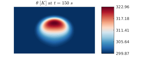
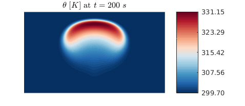
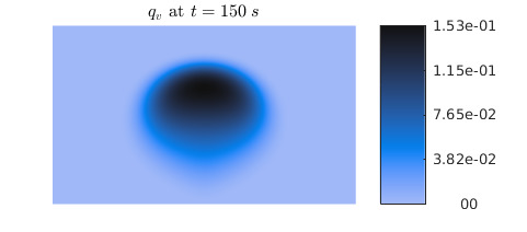
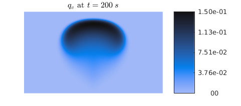
Figure 1. Example 1: Potential temperature $\theta$, water vapor concentration $q_{v}$, cloud drops concentration $q_{c}$ and rain concentration $q_{r}$ at times $t=150$ (left column) and $200s$ (right column) simulated on a $160\times 160$ mesh.

$N$	$L^{2}$-error in $\rho q_{v}$	EOC	$L^{2}$-error in $\rho q_{c}$	EOC	$L^{2}$-error in $\rho q_{r}$	EOC
10	6.870e+00	–	1.019e-01	–	1.159e-03	–
20	1.711e+00	2.01	2.544e-02	2.00	3.152e-04	1.88
40	4.271e-01	2.00	6.380e-03	2.00	1.240e-04	1.35
80	1.080e-01	1.98	1.611e-03	1.99	4.952e-05	1.32
160	2.703e-02	2.00	4.042e-04	1.99	1.571e-05	1.67
320	6.765e-03	2.00	1.016e-04	1.99	5.666e-06	1.47

Table 1. Example 1: $L^{2}$-errors and EOC for the cloud variables computed at time $t=10s$ using $\Delta t=\nicefrac{{20}}{{N}}$.

$N$	$L^{2}$-error in $\rho^{\prime}$	EOC	$L^{2}$-error in $\rho u_{1}$	EOC	$L^{2}$-error in $\rho u_{2}$	EOC	$L^{2}$-error in $(\rho\theta)^{\prime}$	EOC
10	7.522e-01	–	1.134e+02	–	5.805e+01	–	1.213e+02	–
20	1.757e-01	2.10	2.607e+01	2.12	1.744e+01	1.74	3.494e+01	1.80
40	4.418e-02	2.00	5.604e+00	2.22	5.462e+00	1.67	9.641e+00	1.86
80	1.147e-02	1.95	1.436e+00	1.96	1.658e+00	1.72	2.584e+00	1.90
160	3.170e-03	1.85	3.972e-01	1.85	5.875e-01	1.50	7.577e-01	1.77
320	9.810e-04	1.70	1.159e-01	1.78	2.420e-01	1.28	2.556e-01	1.57

Table 2. Example 1: $L^{2}$-errors and EOC for the flow variables computed at time $t=10s$ using $\Delta t=\nicefrac{{20}}{{N}}$.

     

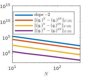
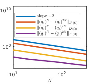
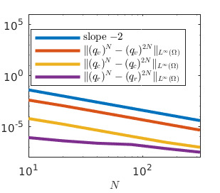
Figure 2. Example 1: Comparison of different error norms for the cloud variables $q_{v}$, $q_{c}$ and $q_{r}$ computed at time $t=10s$ using $\Delta t=\nicefrac{{20}}{{N}}$.

     

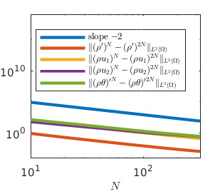
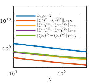
Figure 3. Example 1: Comparison of different error norms for the flow variables $\rho^{\prime}$, $\rho u_{1}$, $\rho u_{2}$ and $(\rho\theta)^{\prime}$ at time $t=10s$ using $\Delta t=\nicefrac{{20}}{{N}}$.

4.2. Rayleigh-Bénard convection

In this experiment, we study a natural convection that is used to model structure formation. It occurs in a planar flow between two horizontal plates, where the lower one is heated from below and the upper one is cooled from above. Due to the presence of buoyancy, and hence gravity, the fluid develops a regular pattern of convection roles, known as the Bénard cells. In 3-D, these convection roles form additionally hexagonal structures; see, e.g., [13, 31, 1].

For our numerical simulations, we prescribe the following initial conditions:

$$\rho^{\prime}(\bm{x},0)=-\bar{\rho}(\bm{x})\frac{\theta^{\prime}(\bm{x},0)}{\bar{\theta}(\bm{x})+\theta^{\prime}(\bm{x},0)},\quad\bar{\rho}(\bm{x})=\frac{p_{0}}{R\bar{\theta}(\bm{x})}\pi_{e}(\bm{x})^{\frac{1}{\gamma-1}},\quad\pi_{e}(\bm{x})=1-\frac{gx_{3}}{c_{p}\bar{\theta}},$$

$$\bm{u}(\bm{x},0)=0,\quad\theta^{\prime}(\bm{x},0)=\eta(\bm{x}),\quad\bar{\theta}(\bm{x})=284-\frac{1}{1000}x_{3},$$

where $p_{0}=\bar{p}=10^{5}\,\mathrm{Pa}$ and $\eta(\bm{x})$ is a random perturbation uniformly distributed in $[-0.0021,0.0021]$. For the cloud equations, the following initial data are used:

$$q_{v}(\bm{x},0)=2\cdot 10^{-5}\bar{\theta}(\bm{x}),\quad q_{c}=0,\quad q_{r}=0.$$

We apply periodic boundary conditions in horizontal direction and the following conditions vertically: $\bm{u}\cdot\bm{n}=0$, $\nabla\rho^{\prime}\cdot\bm{n}=0$, $\nabla(\rho q_{\ell})\cdot\bm{n}=0$, $\ell\in\{v,c,r\}$ with the Dirichlet boundary conditions for the potential temperature,

$$\theta(x_{3}=0)=284\,\mathrm{K}\quad\mbox{and}\quad\theta(x_{3}=1000)=283\,\mathrm{K}.$$

Example 2: 2-D case

In Figures 4–7, we present time snapshots of the numerical solution computed in a domain $\Omega=[0,5000]\times[0,1000]\,\mathrm{m^{2}}$ that has been discretized using $320\times 320$ mesh cells. The potential temperature, water vapor mixing ratio, cloud mass and rain mass concentration are presented at two distinct times ($t=800$ and $1400s$) in Figures 4–7, where we can clearly see the formation and evolution of a pattern. At an earlier time $t=800\,s$, one can observe the formation of small convective cells, visible as narrow finger-like structures reaching towards the top of the domain. Inside these cells, the potential temperature is enhanced, partly due to the upward transport of higher values from below and partly due to phase changes and thus latent heat release. Also the mass concentrations of water vapor and cloud water follow the small scale structure and show enhanced values inside the fingers. Even at this early stage, rain can be formed at the top of the domain, since there the cloud water concentration is high enough for autoconversion and accretion. Nevertheless, the structure of rain water is very different since after the formation of rain, it is vertically transported due to sedimentation leading to vertically smeared structures. By a later time $t=1400\,s$, much larger structures, which are similar to classical structures for dry thermal convection, have been formed. In the variables $\theta$, $q_{v}$ and $q_{c}$, the spatially extended convective cells can be clearly seen. In contrast, rain water is not following the convective structure although some larger features can be seen. In general, smearing due to sedimentation is again a major feature of the rain mass concentration.

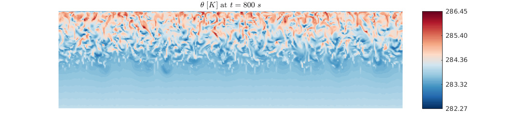
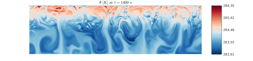
Figure 4. Example 2: Time evolution of the potential temperature $\theta$.

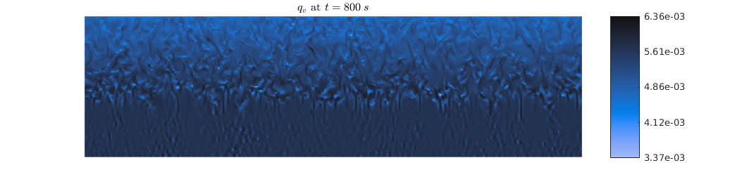
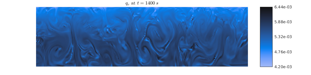
Figure 5. Example 2: Time evolution of the water vapor concentration $q_{v}$.

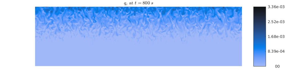
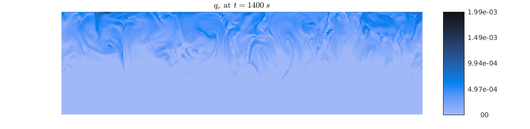
Figure 6. Example 2: Time evolution of the cloud drops concentration $q_{c}$.

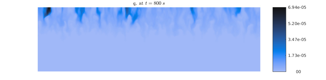
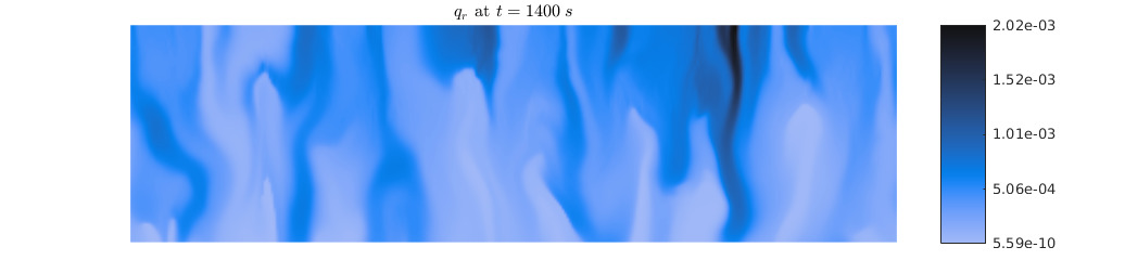
Figure 7. Example 2: Time evolution of the rain concentration $q_{r}$.

Example 3: 3-D case

In this example, we compute the numerical solution in a domain $\Omega=[0,5000]\times[0,5000]\times[0,1000]\,\mathrm{m^{3}}$ that has been discretized using $50\times 50\times 50$ mesh cells. Figures 8–11 show $\theta$, $q_{v}$, $q_{c}$ and $q_{r}$ computed at times $t=1200$, $1600$, $1800$ and $2000s$. In order to better visualize the computed structures, we have plotted the solution in a slightly smaller domain $[0,5000]\times[0,5000]\times[0,980]\,\mathrm{m^{3}}$. As in the 2-D case, different structures are formed in the different variables. At an earlier time $t=1200\,s$, small scale structures can be seen at the top layer of the domain, especially in the potential temperature (Figure 8) and cloud water (Figure 10). As time progresses, these structures aggregate and reorganize to quasi-hexagonal structures, which would be typical for classical dry thermal convection—Rayleigh-Bénard convection. These structures in potential temperature seem to be quite robust as the overall scales and pattern do not change from $t=1800\,s$ to $t=2000\,s$. As one can see in Figure 10, the structures in the cloud water are very similar since the variables $\theta$ and $q_{c}$ are closely connected; the structures are mainly visible in horizontal planes. For the rain distribution, the evolved structures are quite different since rain is formed at regions with high cloud water (that is, at the top layers) and then transported by sedimentation leading to more pronounced pattern in the vertical direction, since sedimentation is the dominant process after the rain has formed.

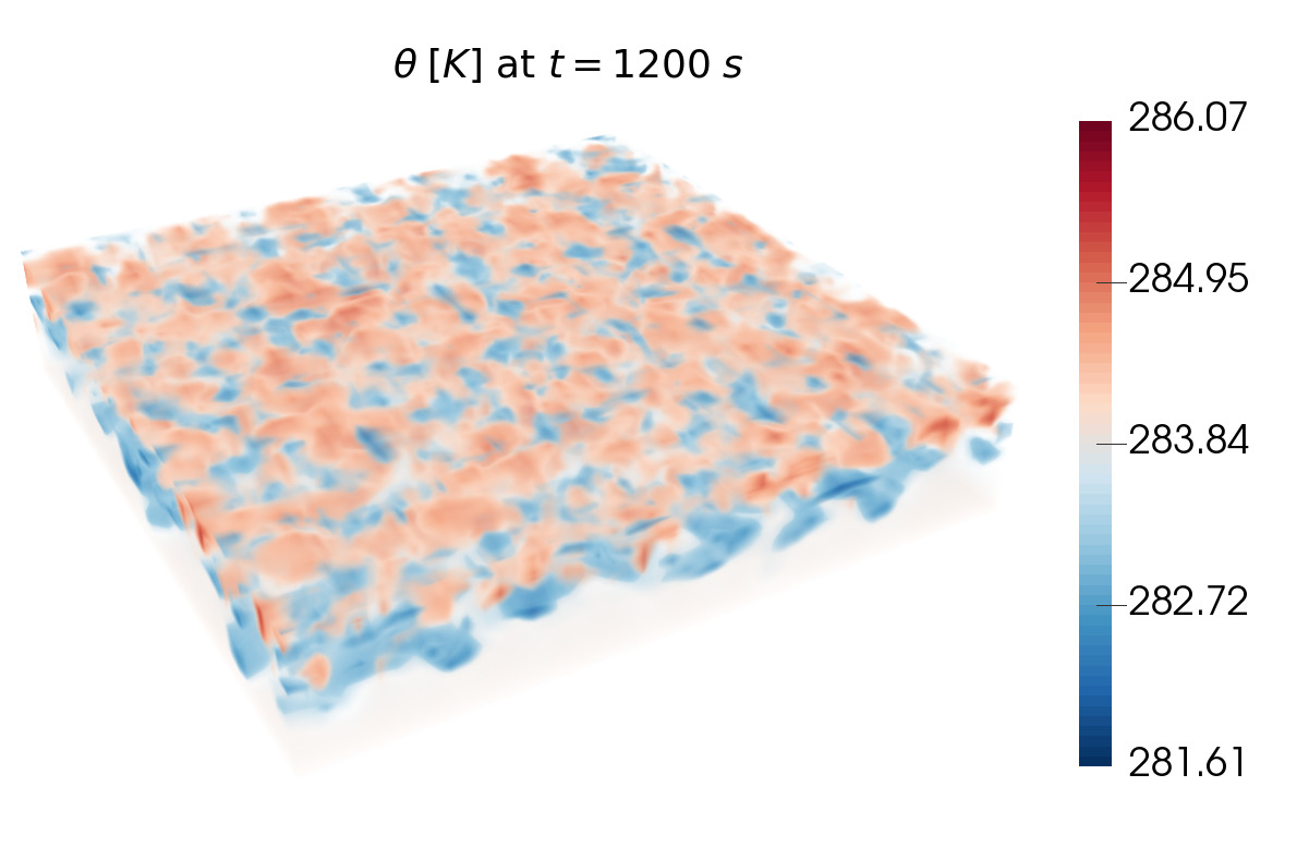
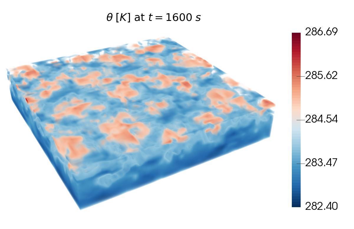
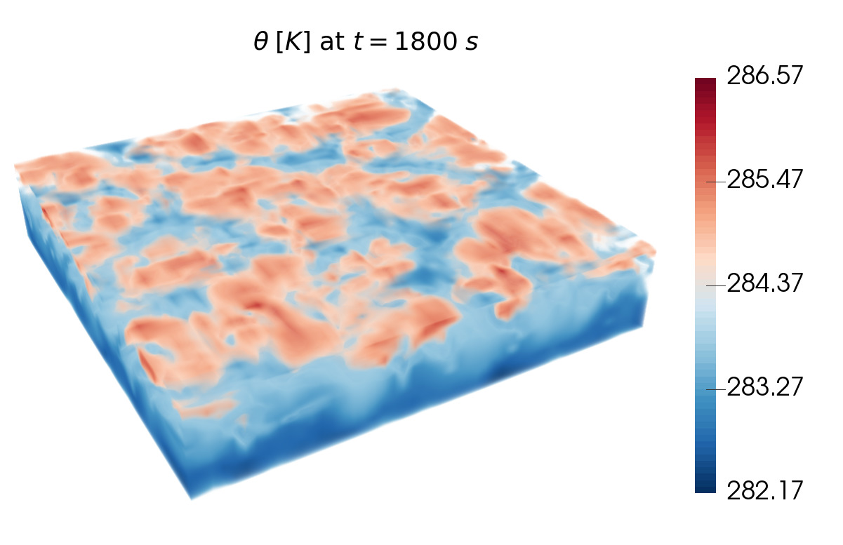
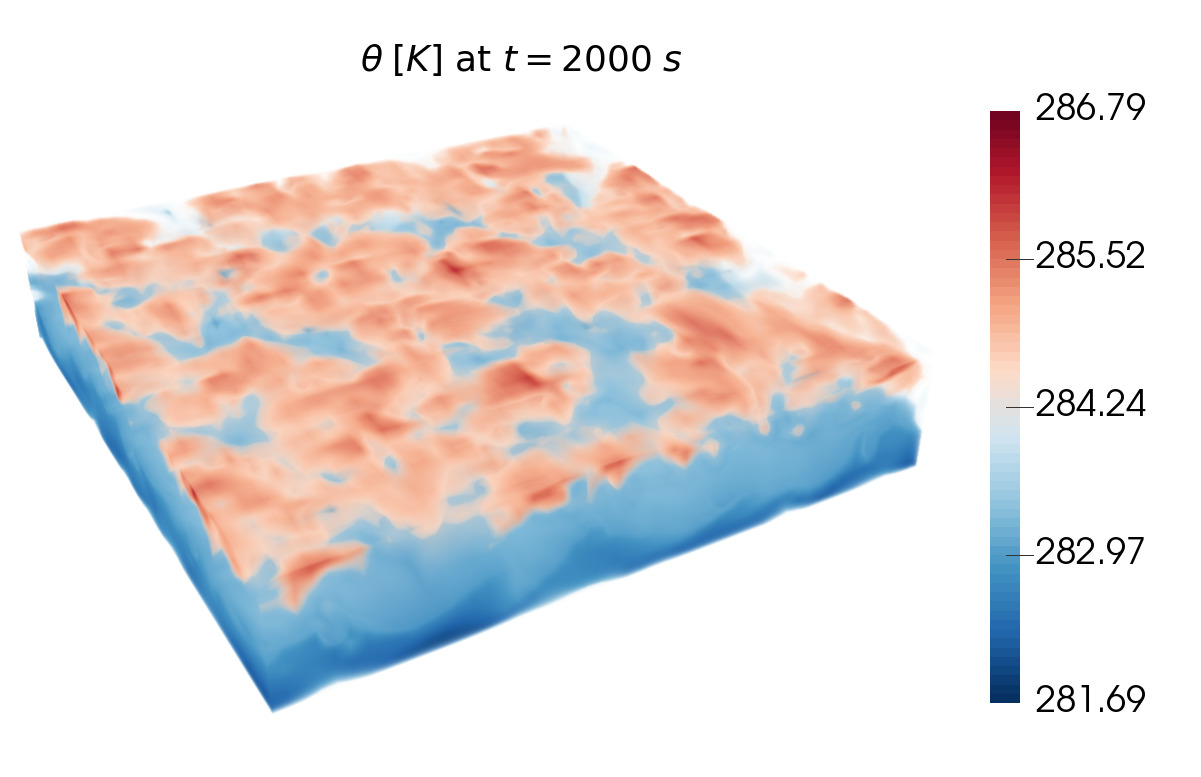
Figure 8. Example 3: Time evolution of the potential temperature $\theta$.

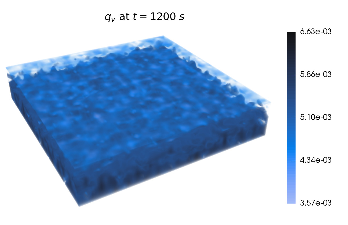
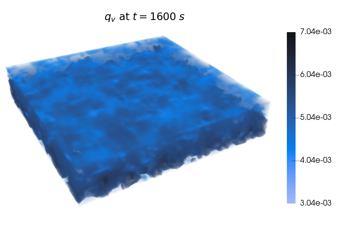
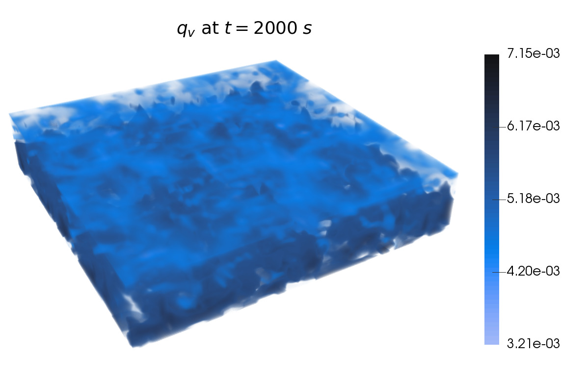
Figure 9. Example 3: Time evolution of the water vapor concentration $q_{v}$.

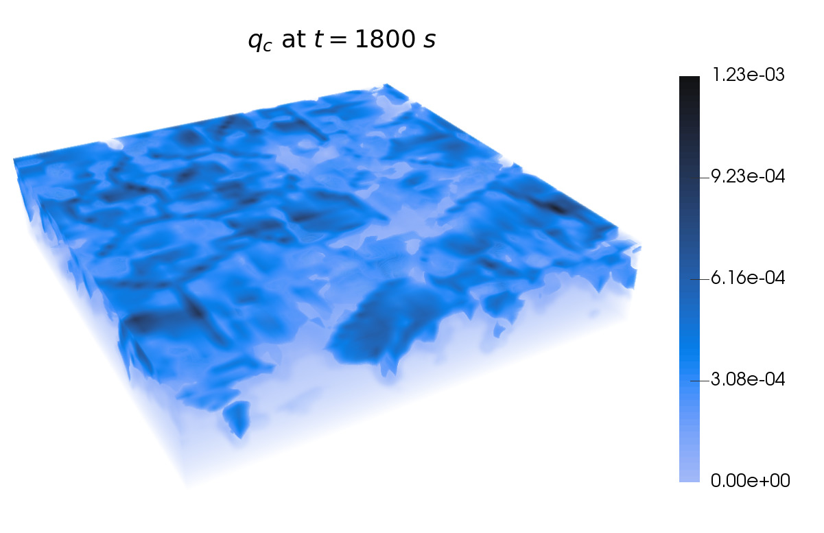
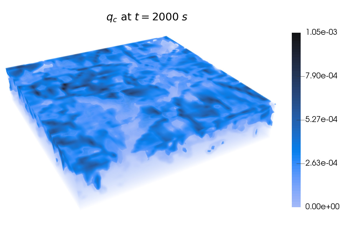
Figure 10. Example 3: Time evolution of the cloud drops concentration $q_{c}$.

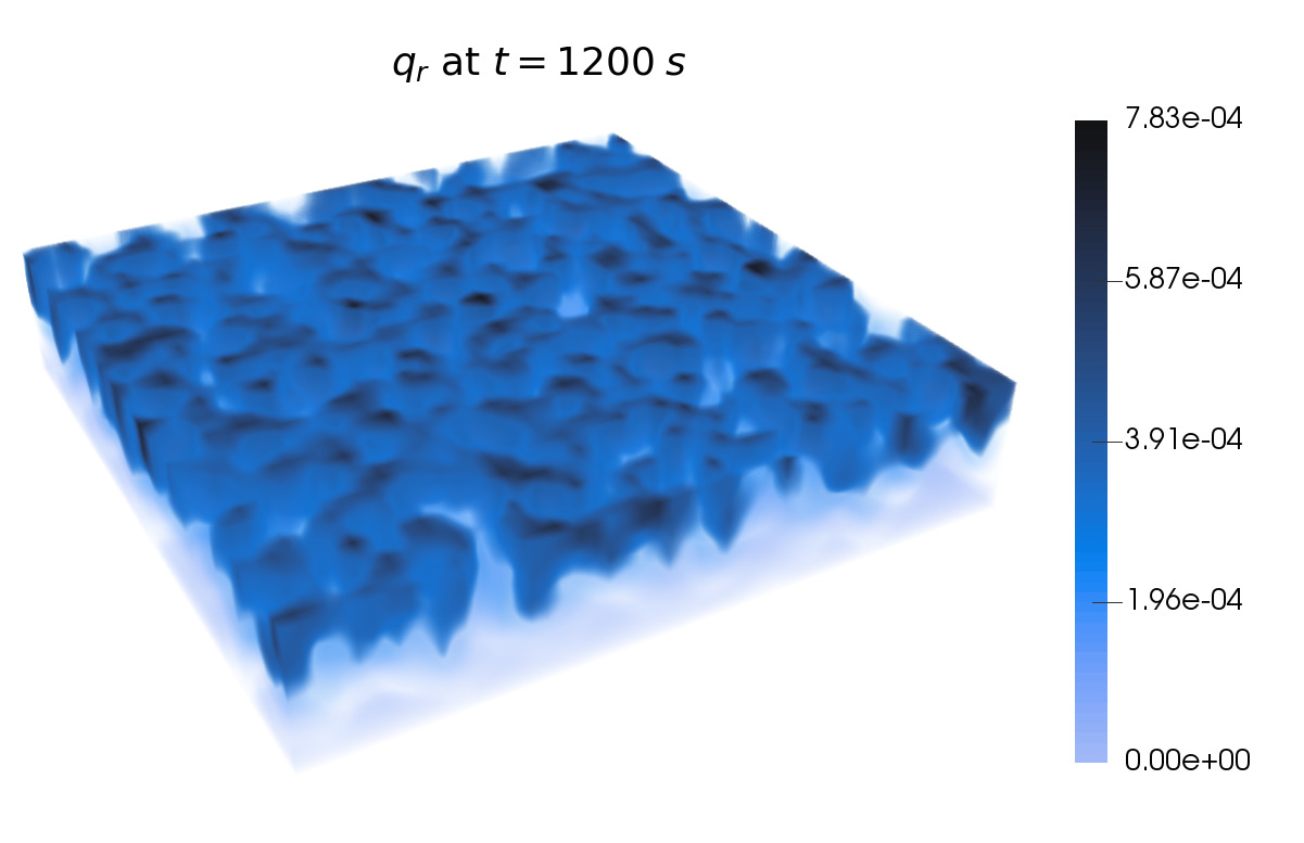
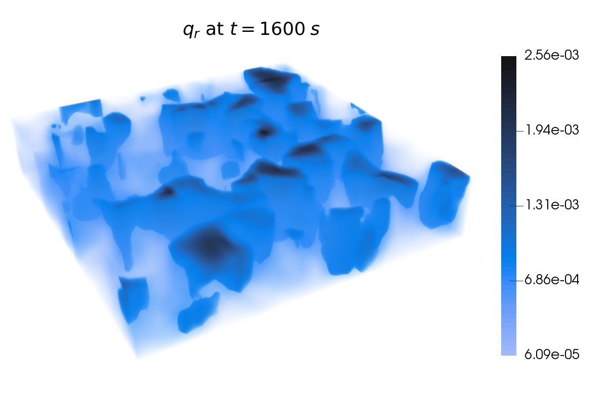
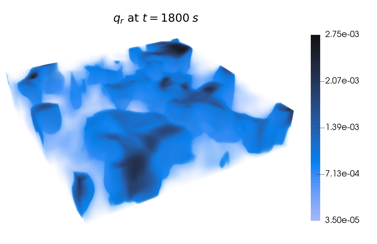
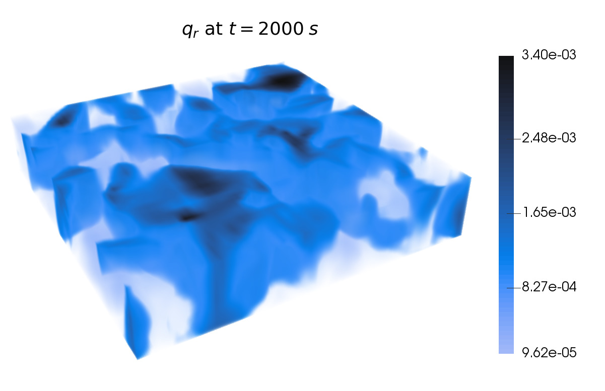
Figure 11. Example 3: Time evolution of the rain concentration $q_{r}$.

Remark 4.1.

Let us note that the Rayleigh-Bénard convection can be understood as a very simplified model for atmospheric convection in the turbulent planetary boundary layer. In [31, 43], numerical simulations for moist Rayleigh-Bénard convection have been realized using the Boussinesq approximation, a simplified equation of state, and the rigid-lid boundary conditions at the top and bottom of the computational domain. Our mathematical model is more general and takes weakly compressible effects into account. Numerical experiments presented in Examples 2 and 3 are in good agreement with the results presented in the literature, but the focus of those studies differs from ours.

5. Stochastic mathematical model

In meteorological applications, it is typical that initial or boundary data as well as parameters are uncertain. In order to take this into account and analyze the influence of such uncertainties on the output of numerical simulations, we apply the stochastic Galerkin method that will be described below. In this paper, we consider the case where the uncertainty arises from the initial data or some coefficients in the microphysical cloud parametrizations. In order to mathematically describe the uncertainty, we introduce a random variable $\omega$. We assume that either the initial data or some well-chosen model parameters depend on $\omega$, that is,

$$(\rho q_{\ell})\big{|}_{t=0}=(\rho q_{\ell})(\bm{x},t=0,\omega)\quad\mbox{with}\quad\ell\in\{v,c,r\}$$

or

$$k_{1}=k_{1}(\omega),\quad k_{2}=k_{2}(\omega),\quad\alpha=\alpha(\omega).$$

Consequently, the solution at later time will also depend on $\omega$, that is, $(\rho q_{\ell})(\bm{x},t,\omega)$ for $\ell\in\{v,c,r\}$, and the system (2) for cloud variables will read as

$$((\rho q_{v})(\omega))_{t}+\nabla\cdot\left((\rho q_{v})(\omega)\bm{u}-\mu_{q}\rho\nabla q_{v}(\omega)\right) =\rho(-C(\omega)+E(\omega)),$$

$$((\rho q_{c})(\omega))_{t}+\nabla\cdot\left((\rho q_{c})(\omega)\bm{u}-\mu_{q}\rho\nabla q_{c}(\omega)\right) =\rho(C(\omega)-A_{1}(\omega)-A_{2}(\omega)),$$ (5.1)

$$((\rho q_{r})(\omega))_{t}+\nabla\cdot\left((\rho q_{r})(\omega)(-v_{q}(\omega)\bm{e_{3}}+\bm{u})-\mu_{q}\rho\nabla q_{r}(\omega)\right) =\rho(A_{1}(\omega)+A_{2}(\omega)-E(\omega)).$$

From now on we will stress the dependence on $\omega$, but we will omit the dependence on $\bm{x}$ and $t$ to simplify the notation. We would like to point out that the solution of the Navier-Stokes equations (2.2) will also depend on $\omega$, because of the source term $S_{\theta}$. In this paper, we will consider a simplified situation by replacing

$$S_{\theta}(\omega)=\rho\frac{L\theta}{c_{p}T}\big{\{}C((\rho q_{v})(\omega),(\rho q_{c})(\omega))-E((\rho q_{v})(\omega),(\rho q_{r})(\omega))\big{\}}$$

in (2.2) by $\bar{S}_{\theta}$ which only depends on the expected values of the cloud variables

$$\bar{S}_{\theta}:=\rho\frac{L\theta}{c_{p}T}\big{\{}C(\mathbb{E}[\rho q_{v}],\mathbb{E}[\rho q_{c}])-E(\mathbb{E}[\rho q_{v}],\mathbb{E}[\rho q_{r}])\big{\}}.$$

This ensures that all of the fluid variables, $\rho^{\prime}$, $\rho\bm{u}$ and $(\rho\theta)^{\prime}$, remain deterministic.

6. Numerical scheme for the stochastic model

In this section, we describe a generalized polynomial chaos stochastic Galerkin (gPC-SG) method for the system of cloud equations (5). Such method belongs to the class of intrusive methods and the use of the Galerkin expansion leads to a system of deterministic equations for the expansion coefficients. In the gPC-SG method, the solution is sought in the form of a polynomial expansion

$$\rho q_{\ell}(\bm{x},t,\omega)=\sum_{k=0}^{M}(\widehat{\rho q_{\ell}})_{k}(\bm{x},t)\Phi_{k}(\omega)\quad\mbox{with}\quad\ell\in\{v,c,r\},~{}M\geq 0,$$ (6.1)

where $\Phi_{k}(\omega)$, $k=0,\ldots,M$, are polynomials of $k$-th degree that are orthogonal with respect to the probability density function $\mu(\omega)$. The choice of the orthogonal polynomials $\{\Phi_{k}(\omega)\}_{k=0}^{M}$ depends on the distribution of $\omega$. In our case, we use a uniformly distributed $\omega\in\Gamma=(-1,1)$, which defines the Legendre polynomials, which satisfy

$$\int\limits_{\Gamma}\Phi_{k}(\omega)\Phi_{k^{\prime}}(\omega)\mu(\omega)\,{\rm d}\omega={\color[rgb]{0,0,0}\frac{1}{2k+1}}\delta_{kk^{\prime}}\quad\mbox{for}\quad 0\leq k,k^{\prime}\leq M,$$ (6.2)

where $\delta_{kk^{\prime}}$ is the Kronecker symbol and $\Gamma$ is the sample space.

We use the same expansion for the uncertain coefficients,

$$k_{1}(\omega)=\sum_{k=0}^{M}(\widehat{k_{1}})_{k}\Phi_{k}(\omega),\quad k_{2}(\omega)=\sum_{k=0}^{M}(\widehat{k_{2}})_{k}\Phi_{k}(\omega),\quad\alpha(\omega)=\sum_{k=0}^{M}\widehat{\alpha}_{k}\Phi_{k}(\omega),$$ (6.3)

for the source terms on the RHS of (5),

$$\rho\left(-C(\bm{x},t,\omega)+E(\bm{x},t,\omega)\right)=:R_{1}(\bm{x},t,\omega) =\sum_{k=0}^{M}(\widehat{r_{1}})_{k}(\bm{x},t)\Phi_{k}(\omega),$$

$$\rho\left(C(\bm{x},t,\omega)-A_{1}(\bm{x},t,\omega)-A_{2}(\bm{x},t,\omega)\right)=:R_{2}(\bm{x},t,\omega) =\sum_{k=0}^{M}(\widehat{r_{2}})_{k}(\bm{x},t)\Phi_{k}(\omega),$$ (6.4)

$$\rho\left(A_{1}(\bm{x},t,\omega)+A_{2}(\bm{x},t,\omega)-E(\bm{x},t,\omega)\right)=:R_{3}(\bm{x},t,\omega) =\sum_{k=0}^{M}(\widehat{r_{3}})_{k}(\bm{x},t)\Phi_{k}(\omega),$$

as well as for the raindrop fall velocity,

$$v_{q}(\bm{x},t,\omega)=\sum_{k=0}^{M}(\widehat{v_{q}})_{k}(\bm{x},t)\Phi_{k}(\omega).$$ (6.5)

Since $\rho(\bm{x},t)=\widehat{\rho}_{0}(\bm{x},t)$, we also obtain

$$q_{\ell}(\bm{x},t,\omega)=\sum_{k=0}^{M}(\widehat{q_{\ell}})_{k}(\bm{x},t)\Phi_{k}(\omega)\quad\mbox{with}\quad(\widehat{q_{\ell}})_{k}(\bm{x},t)=\frac{(\widehat{\rho q_{\ell}})_{k}(\bm{x},t)}{\rho(\bm{x},t)}~{}~{}~{}\mbox{for}~{}\ell\in\{v,c,r\},~{}k=1,\ldots,M.$$ (6.6)

We note that if $\rho(\bm{x},t)$ is very small, the computation of the coefficients $(\widehat{q_{\ell}})_{k}(\bm{x},t)$ should be desingularized; see [20, formulae (5.16)–(5.18)].

Applying the Galerkin projection to (5) yields

$$\left\langle(\rho q_{v})_{t}+\nabla\cdot\left(\rho q_{v}\bm{u}-\mu_{q}\rho\nabla q_{v}\right),\Phi_{k}\right\rangle =\left\langle\rho(-C+E),\Phi_{k}\right\rangle,$$

$$\left\langle(\rho q_{c})_{t}+\nabla\cdot\left(\rho q_{c}\bm{u}-\mu_{q}\rho\nabla q_{c}\right),\Phi_{k}\right\rangle =\left\langle\rho(C-A_{1}-A_{2}),\Phi_{k}\right\rangle,$$ (6.7)

$$\left\langle(\rho q_{r})_{t}+\nabla\cdot\left(\rho q_{r}(-v_{q}\bm{e_{3}}+\bm{u})-\mu_{q}\rho\nabla q_{r}\right),\Phi_{k}\right\rangle =\left\langle\rho(A_{1}+A_{2}-E),\Phi_{k}\right\rangle,$$

for $k=0,\ldots,M$, where $\langle\cdot,\cdot\rangle$ is the scalar product in our probability space which is given through

$$\langle u,v\rangle=\int\limits_{-1}^{1}u(\omega)v(\omega)\mu(\omega)\,{\rm d}\omega.$$

We now substitute (6.1), (6)–(6.6) into (6) and use the orthogonality property (6.2) to obtain the following $3(M+1)\times 3(M+1)$ deterministic system for the gPC coefficients:

$$\frac{\partial}{\partial t}(\widehat{\rho q_{v}})_{k}+\sum_{s=1}^{d}\frac{\partial}{\partial x_{s}}\left((\widehat{\rho q_{v}})_{k}u_{s}\right)-\mu_{q}\sum_{s=1}^{d}\left(\frac{\partial\rho}{\partial x_{s}}\frac{\partial}{\partial x_{s}}(\widehat{q_{v}})_{k}+\rho\frac{\partial^{2}}{\partial x_{s}^{2}}(\widehat{q_{v}})_{k}\right) =(\widehat{r_{1}})_{k},$$

$$\frac{\partial}{\partial t}(\widehat{\rho q_{c}})_{k}+\sum_{s=1}^{d}\frac{\partial}{\partial x_{s}}\left((\widehat{\rho q_{c}})_{k}u_{s}\right)-\mu_{q}\sum_{s=1}^{d}\left(\frac{\partial\rho}{\partial x_{s}}\frac{\partial}{\partial x_{s}}(\widehat{q_{c}})_{k}+\rho\frac{\partial^{2}}{\partial x_{s}^{2}}(\widehat{q_{c}})_{k}\right) =(\widehat{r_{2}})_{k},$$ (6.8)

$$\frac{\partial}{\partial t}(\widehat{\rho q_{r}})_{k}-\frac{\partial}{\partial x_{d}}\widehat{\alpha}_{k}+\sum_{s=1}^{d}\frac{\partial}{\partial x_{s}}\left((\widehat{\rho q_{r}})_{k}u_{s}\right)-\mu_{q}\sum_{s=1}^{d}\left(\frac{\partial\rho}{\partial x_{s}}\frac{\partial}{\partial x_{s}}(\widehat{q_{r}})_{k}+\rho\frac{\partial^{2}}{\partial x_{s}^{2}}(\widehat{q_{r}})_{k}\right) =(\widehat{r_{3}})_{k},$$

for $k=0,\ldots,M$. Here, the coefficients $\{\widehat{\alpha}_{k}\}_{k=0}^{M}$ are obtained using the following expansion:

$$v_{q}(\bm{x},t,\omega)(\rho q_{r})(\bm{x},t,\omega)=\sum_{j=0}^{M}(\widehat{v_{q}})_{j}(\bm{x},t)\Phi_{j}(\omega)\sum_{m=0}^{M}(\widehat{\rho q_{r}})_{m}(\bm{x},t)\Phi_{m}(\omega)=:\sum_{k=0}^{M}\widehat{\alpha}_{k}(\bm{x},t)\Phi_{k}(\omega).$$

The coefficients $\{(\widehat{r_{1}})_{k},(\widehat{r_{2}})_{k},(\widehat{r_{3}})_{k}\}_{k=0}^{M}$, as well as $\{\widehat{\alpha}_{k}\}_{k=0}^{M}$ are calculated via discrete Legendre transform (DLT) and inverse discrete Legendre transform (IDLT), which can be briefly described as follows.

• DLT: First, the Galerkin projection applied to the expansion $f(\bm{x},t,\omega)=\sum_{k=0}^{M}\widehat{f}_{k}(\bm{x},t)\Phi_{k}(\omega)$ yields

  $$\widehat{f}_{k}(\bm{x},t)=\frac{2k+1}{2}\int\limits_{-1}^{1}f(\bm{x},t,\omega)\Phi_{k}(\omega)\,{\rm d}\omega\quad\mbox{for}\quad 0\leq k\leq M.$$ (6.9)

  Then, approximating the integral in (6.9) using the Gauss-Legendre quadrature leads to

  $$\mbox{DLT}\left[\left\{f(\bm{x},t,\omega_{\ell})\right\}_{\ell=0}^{M}\right]=\left\{\widehat{f}_{k}(\bm{x},t)\right\}_{k=0}^{M}=\left\{\frac{2k+1}{2}\sum_{l=0}^{M}\beta_{\ell}f(\bm{x},t,\omega_{\ell})\Phi_{k}(\omega_{\ell})\right\}_{k=0}^{M},$$

  where $\beta_{\ell}$ are the Gauss-Legendre quadrature weights and $\omega_{\ell}$ is the $\ell$-th root of $\Phi_{M+1}$.

• IDLT: Given the coefficients $\{\widehat{f}_{k}\}_{k=0}^{M}$, we compute the function $f$ through the gPC expansion

  $$\mbox{IDLT}\left[\left\{\widehat{f}_{k}(\bm{x},t)\right\}_{k=0}^{M}\right]=\left\{f(\bm{x},t,\omega_{\ell})\right\}_{l=0}^{M}=\left\{\sum_{k=0}^{M}\widehat{f}_{k}(\bm{x},t)\Phi_{k}(\omega_{\ell})\right\}_{\ell=0}^{M}.$$

Consequently, we obtain

$$\{(\widehat{r_{1}})_{k}\}_{k=0}^{M}=\mbox{DLT}\left[R_{1}\left(\mbox{IDLT}\left[\left\{(\widehat{\rho q_{v}})_{k}\right\}_{k=0}^{M}\right],\mbox{IDLT}\left[\left\{(\widehat{\rho q_{c}})_{k}\right\}_{k=0}^{M}\right],\mbox{IDLT}\left[\left\{(\widehat{\rho q_{r}})_{k}\right\}_{k=0}^{M}\right]\right)\right],$$

and analogously for $\{(\widehat{r_{2}})_{k}\}_{k=0}^{M}$, $\{(\widehat{r_{3}})_{k}\}_{k=0}^{M}$ and $\{\widehat{\alpha}_{k}\}_{k=0}^{M}$.

Remark 6.1.

We stress that since the values $\Phi_{k}(\omega_{\ell})$, $0\leq k,\ell\leq M$, are needed every time either DLT or IDLT is applied, one can pre-compute them for the code efficiency.

For the spatial and temporal discretizations of the system (6), we apply the same finite volume method as described in Section 3.2 and the same large stability domain explicit time integration method mentioned in Section 3.3. As in the deterministic case, we implement the ODE solver DUMKA3, which we provide with the following time step stability restriction for the forward Euler method:

$$\max_{s=1,2}\,\max_{i=1,\ldots,N}(|(u_{s})_{i}|,|(u_{3})_{i}+v_{q}(\omega_{l})|)\,\frac{\Delta t^{n}_{\rm cloud}}{h}<0.5,$$

which should be satisfied for all of the Legendre roots $\omega_{\ell}$, $\ell={\color[rgb]{0,0,0}0},\ldots,M$.

7. Stochastic numerical experiments

In this section, we conduct numerical experiments with the stochastic Galerkin method described in Section 6 for the free convection of a moist warm air bubble and the Rayleigh-Bénard convection. We demonstrate the influence of uncertainty in initial data as well as in cloud parameters on the solution of the coupled Navier-Stokes-cloud model (2.2), (5). In all of our numerical examples below, we take $M=3$. Our extensive tests, from which we present here only a selected part, showed that this was sufficient. Indeed, as documented in Example 6, high-order stochastic coefficients typically have very small influence on a solution (see Figure 15), and thus can be neglected. Similar behavior was observed in other experiments.

7.1. Free convection of a smooth warm air bubble

In this test, we modify Example 1 by randomly perturbing either the initial data or selected model parameters.

Example 4: 2-D case with stochastic initial data

We begin by considering the following experiment with a $10\%$ perturbation of the initial water vapor concentration:

$$(\widehat{q_{v}})_{0}(\bm{x},0) =0.02\theta^{\prime}(\bm{x},0),~{}~{}~{}(\widehat{q_{v}})_{1}(\bm{x},0)=0.1(\widehat{q_{v}})_{0}(\bm{x},0),~{}~{}~{}(\widehat{q_{v}})_{k}(\bm{x},0)=0\quad\mbox{for}\quad 2\leq k\leq M,$$

$$(\widehat{q_{c}})_{k}(\bm{x},0) =(\widehat{q_{r}})_{k}(\bm{x},0)=0\quad\mbox{for}\quad 0\leq k\leq M.$$

We compute the solution using different meshes until the final time $t=10s$.

The experimental convergence study for the cloud and flow variables is presented in Figure 12. Similarly to the deterministic case, one can observe second-order convergence in space and time. In order to test the convergence in the stochastic space, we obtain a reference solution computed by the stochastic Galerkin method with 20 stochastic modes. The convergence study is presented in Figure 13, where we plot the difference between the approximate and reference solutions, both computed using a mesh with $160\times 160$ cells and $\Delta t=0.01$ at time $t=10s$. One can clearly see a spectral convergence with the rate $e^{-0.3M}$.

              

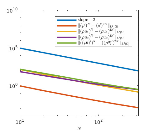
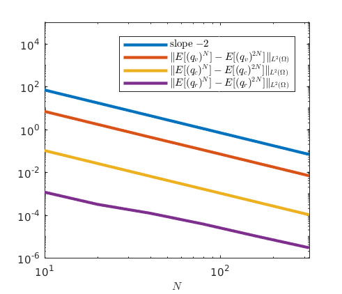
Figure 12. Example 4: Convergence study for the flow variables (left) and the expected values of $(\rho q_{\ell})_{k}$, $\ell\in\{v,c,r\}$ (right) in space and time.

     

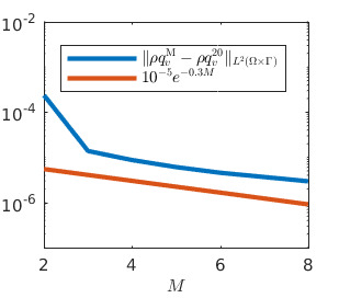
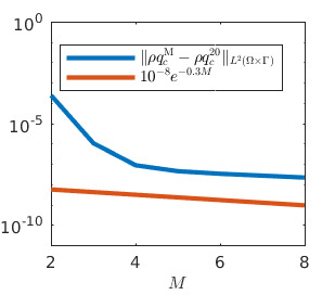
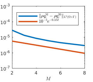
Figure 13. Example 4: Convergence study for the cloud variables $(\rho q_{\ell})$, $\ell\in\{v,c,r\}$ in the stochastic space.

Example 5: 2-D case with stochastic parameters

In this experiment, we perturb the three selected model parameters ($k_{1}$, $k_{2}$ and $\alpha$) by $50\%$ each:

$$(\widehat{k_{1}})_{0} =0.0041,\quad(\widehat{k_{1}})_{1}=0.5(\widehat{k_{1}})_{0},\quad(\widehat{k_{1}})_{k}=0\quad\mbox{for}\quad 2\leq k\leq M,$$

$$(\widehat{k_{2}})_{0} =0.8,\quad(\widehat{k_{2}})_{1}=0.5(\widehat{k_{2}})_{0},\quad(\widehat{k_{2}})_{k}=0\quad\mbox{for}\quad 2\leq k\leq M,$$

$$\widehat{\alpha}_{0} =190.3,\quad\widehat{\alpha}_{1}=0.5\widehat{\alpha}_{0},\quad\widehat{\alpha}_{k}=0\quad\mbox{for}\quad 2\leq k\leq M.$$

These parameters were proposed in [34] as the most sensitive model parameters. We study the convergence in the stochastic space. To this end, we plot in Figure 14 the difference between the approximate and reference (obtained with 20 stochastic modes) solutions, both computed using a mesh with $160\times 160$ cells and $\Delta t=0.01$ at time $t=10s$. As in Example 4, one can observe a spectral convergence with the rate $e^{-0.3M}$.

     

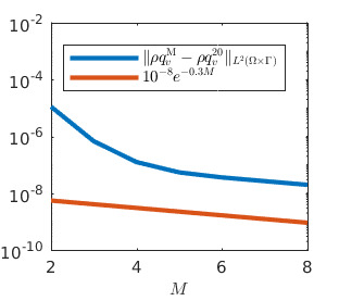
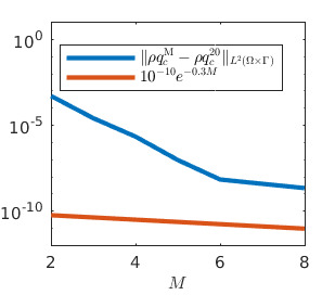
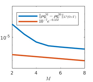
Figure 14. Example 5: Convergence study for the cloud variables $(\rho q_{\ell})$, $\ell\in\{v,c,r\}$ in the stochastic space.

Example 6: Comparison of the stochastic Galerkin and stochastic collocation methods in the 3-D case

In this comparison test, we consider free convection of a moist smooth warm air bubble with perturbed initial data as in Example 4. Numerical solutions are computed on $50\times 50\times 50$ mesh at time $t=1s$. We compare the performance of the stochastic Galerkin and stochastic collocation methods. The collocation method (see, e.g., [8]) is an interpolation method in the stochastic space, which uses a deterministic model with the values of the stochastic variable taken at collocation points suitably chosen on the interval $(-1,1)$; here, we use the Gauss-Legendre points.

In Figure 15, the $L^{2}$-norms of the stochastic coefficients of the stochastic Galerkin ($\|(\widehat{\rho q_{\ell}})_{m}\|_{L^{2}(\Omega)}$) and stochastic collocation ($\|(\widetilde{\rho q_{\ell}})_{m}\|_{L^{2}(\Omega)}$) methods for $\ell\in\{v,c,r\}$ and $m=0,\ldots,19$ are shown. One can observe an exponential decay with respect to $m$ and good agreement between both methods that demonstrates the reliability of the stochastic Galerkin method. We note, however, that the norms of the solutions computed by these two different methods are not equal since the stochastic Galerkin method uses the expected values of the cloud variables in the Navier-Stokes equations.

     

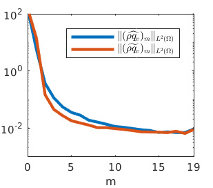
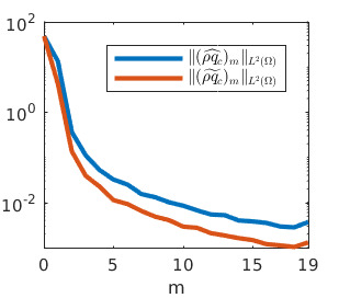
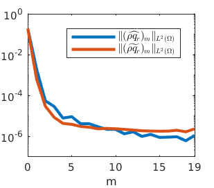
Figure 15. Example 6: $L^{2}(\Omega)$-norms of the stochastic coefficients computed by the stochastic Galerkin ($(\widehat{\rho q_{\ell}})_{m}$) and stochastic collocation ($(\widetilde{\rho q_{\ell}})_{m}$) methods, $\ell\in\{v,c,r\}$.

In Figure 16, we compare the CPU times consumed by the stochastic Galerkin and stochastic collocation methods with the same number $M$ of stochastic modes/collocation points. Since the stochastic Galerkin method solves the Navier-Stokes equations just once instead of $M$ times, as needed by the stochastic collocation method does, it is expected to outperform the stochastic collocation method. This has been confirmed by our simulations.

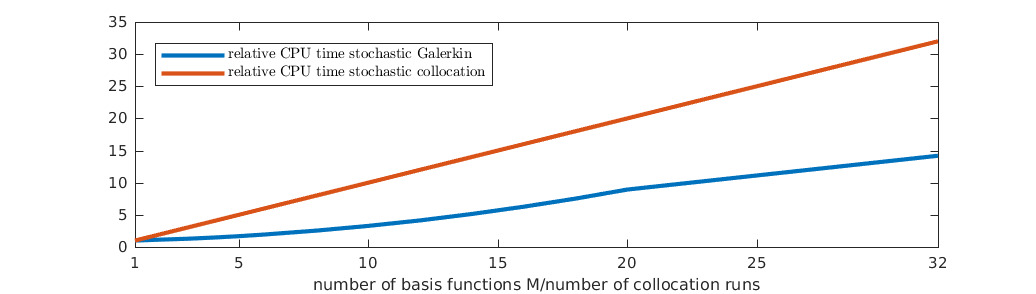
Figure 16. Example 6: Relative CPU times consumed by the stochastic Galerkin and stochastic collocation methods.

7.2. Rayleigh-Bénard convection

In this section, we present results of uncertainty study for the Rayleigh-Bénard convection in both 2-D and 3-D. We investigate uncertainty propagation, which is triggered either by the initial data or cloud parameters.

Example 7: 2-D case with stochastic initial data

In this experiment, we choose the same initial data for the flow variables as in Section 4.2 and perturb the initial data in $q_{v}$ by $5\%$, $10\%$, $20\%$ and $50\%$:

$$(\widehat{q_{v}})_{0}(\bm{x},0) =2\cdot 10^{-5}\bar{\theta},\,(\widehat{q_{v}})_{1}(\bm{x},0)=\nu(\widehat{q_{v}})_{0}(\bm{x},0),\,(\widehat{q_{v}})_{k}=0\quad\mbox{for}\quad 2\leq k\leq M,$$ (7.1)

$$(\widehat{q_{c}})_{k}(\bm{x},0) =(\widehat{q_{r}})_{k}(\bm{x},0)=0\quad\mbox{for}\quad 0\leq k\leq M,$$

where $\nu=0.05$, $0.1$, $0.2$ and $0.5$, respectively. It should be observed that uniform perturbations in the initial conditions for $q_{v}$ may lead to either reduced or enhanced water vapor concentrations as compared to the deterministic simulations. Since the temperature gradient is quite small, a change in $q_{v}$ translates to an (almost) linear change in saturation ratio, which directly controls cloud formation. Thus, in the case of positive perturbations, a higher water vapor concentration leads to earlier cloud formation and, in addition, a higher potential temperature change since more water is available in the system. On the other hand, lower values of $q_{v}$ lead to a time delay in the formation of clouds, even if small convective cells are driven by the dry unstable situation. In a feedback cycle, a reduced or even delayed formation of cloud water propagates further to a weaker rain formation. Finally, the evaporation of rain water leads to a strong cooling effect of the lower layers of the domain, which also crucially depends on the amount of sedimenting rain water. These effects have to be taken into account for the evaluation of the different perturbation scenarios.

Numerical solutions for both the potential temperature $\theta$ (Figure 17) and the expected value of the cloud drops concentration $q_{c}$ (Figure 18) are computed at time $t=1400s$ using $320\times 320$ mesh cells and presented for $\nu=0$, $0.05$, $0.1$, $0.2$ and $0.5$. For a better comparison, we have used the same range of values for different perturbations in all of the plots.

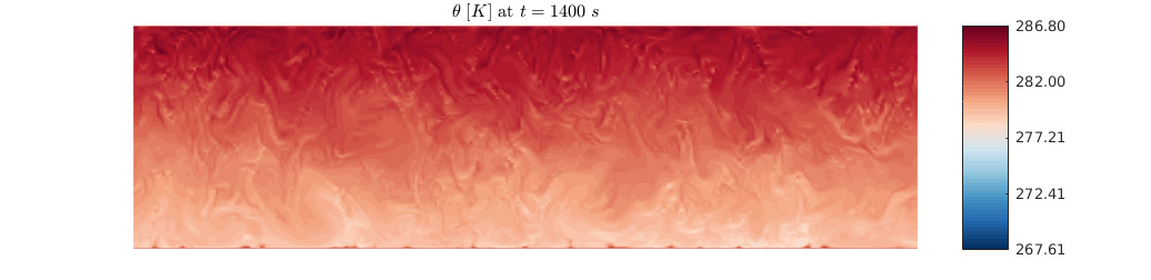
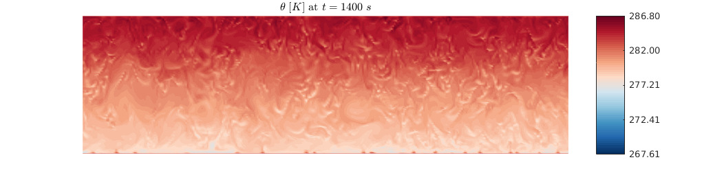
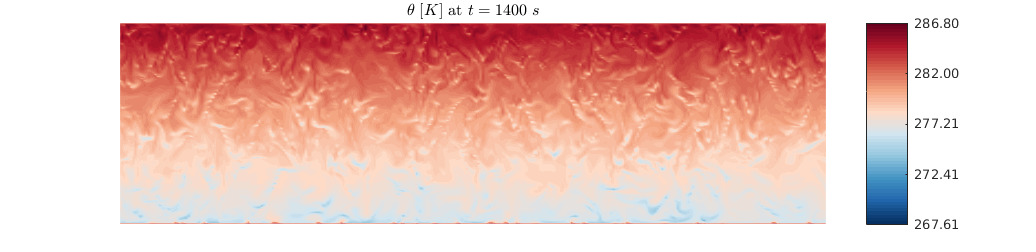
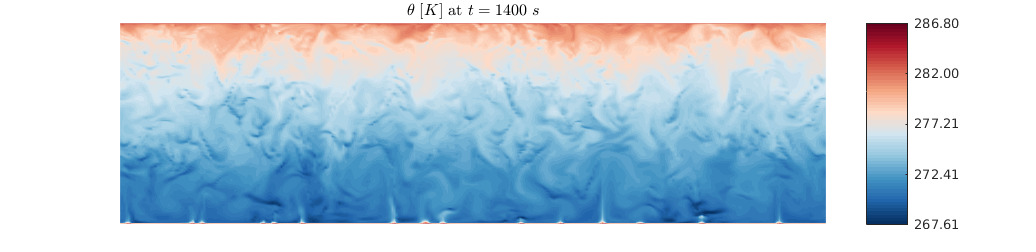
Figure 17. Example 7: Potential temperature $\theta$ for $\nu=0$, $0.05$, $0.1$, $0.2$ and $0.5$ (from top to down).

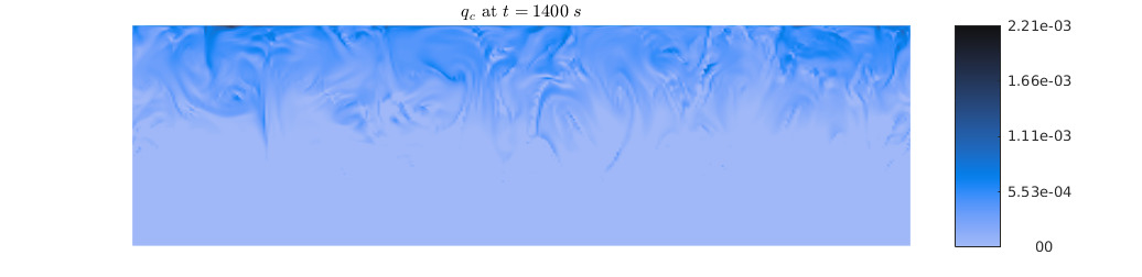
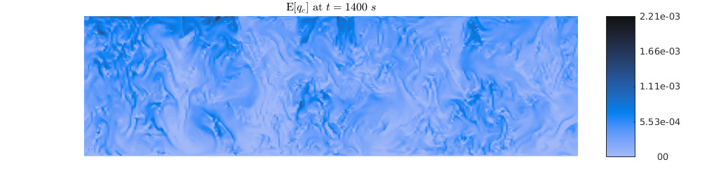
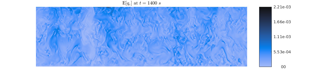
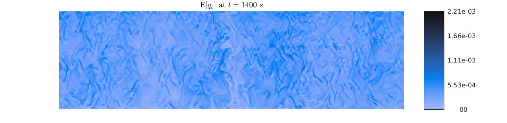
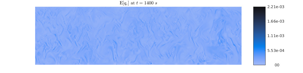
Figure 18. Example 7: Cloud drops concentration $q_{c}$ for $\nu=0$, $0.05$, $0.1$, $0.2$ and $0.5$ (from top to down).

From the results shown in Figure 17 for the potential temperature $\theta$, one can observe two major features that increase in strength with increasing strength of perturbations. First, larger perturbations lead to more concise fine structures, that is, for the deterministic simulation ($\nu=0$), the variable is quite smooth, whereas for large perturbations, large gradients on a very small scale appear. This feature can also be recognized for the cloud water, that is, for the expected values $\mathbb{E}[q_{c}]$ of cloud water concentrations in Figure 18. This is probably due to the fact that even small variations in water vapor have a strong impact on cloud formation, since the activation of cloud droplet is basically a threshold process. For values closer to saturation, even small variations in vertical upward motions can trigger cloud formation. Thus, the small scale variations are more prominent in the massively perturbed scenarios. The second feature is even more striking. Increasing the perturbation in the initial water vapor distribution leads to a stronger vertical gradient in potential temperature, that is, at low levels the temperature is much smaller than in the deterministic case. This feature is due to cooling of sedimenting rain water. For simulations with a high water vapor loading, more cloud and thus more rain is formed, which is subsequently falling down into lower levels and cools the environment by evaporation. Since this process is very effective, the temperature can be reduced drastically. Note that this feature is well-known for the real atmosphere: Falling rain can cool lower levels efficiently, so that a transition from melting rain droplets to snow can be possible for winter seasons. The efficient formation of rain also leads to a strong reduction in cloud water, since accretion can eat up cloud droplets in the lower level; see Figure 18. For reduced values of initial water vapor, processes of cloud and precipitation formation is strongly reduced. However, on average the positive perturbations dominate the statistical picture.

In Figure 19, we plot the standard deviation of the cloud drops concentration. Here, we compute the standard deviation for a function $f(\bm{x},t,\omega)=\sum_{k=0}^{M}\widehat{f_{k}}(\bm{x},t)\Phi_{k}(\omega)$ as

$$\sigma(f(\bm{x},t,\omega))=\sqrt{\sum_{k=1}^{M}\frac{1}{2k+1}\widehat{f_{k}}(\bm{x},t)^{2}},$$ (7.2)

which follows from the orthogonal property (6.2).

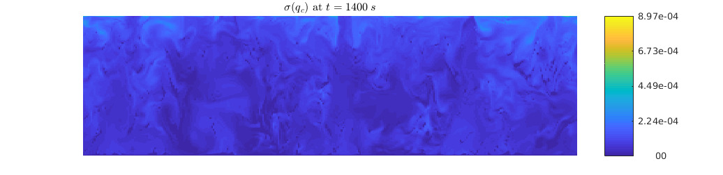
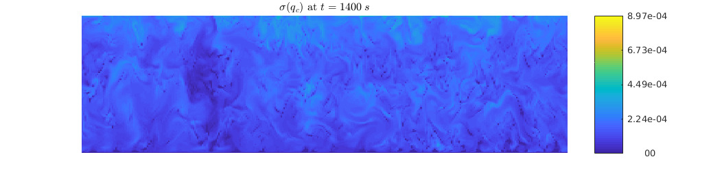
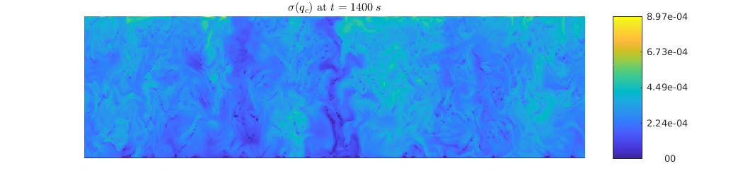
Figure 19. Example 7: Standard deviation of the cloud drops concentration $q_{c}$ for $\nu=0.05$, $0.1$, $0.2$ and $0.5$ (from top to down).

In order to investigate the influence of perturbations, the time evolution of the mean expected value per $m^{2}$ as well as the mean standard deviation per $m^{2}$ for the cloud variables are presented in Figure 20. In $d$-space dimensions these quantities can be computed in the following way:

$$\mathbb{E}\left[\frac{h^{d}}{|\Omega|}\sum_{i=1}^{N}(q_{\ell})_{i}\right] =\frac{h^{d}}{|\Omega|}\sum_{i=1}^{N}\mathbb{E}\left[(q_{\ell})_{i}\right]=\frac{h^{d}}{|\Omega|}\sum_{i=1}^{N}\widehat{((q_{\ell})_{i})_{0}},$$

$$\sigma\left(\frac{h^{d}}{|\Omega|}\sum_{i=1}^{N}(q_{\ell})_{i}\right) =\frac{h^{d}}{|\Omega|}\sqrt{\sum_{k=1}^{M}\left(\sum_{i=1}^{N}\widehat{((q_{\ell})_{i})_{k}}\right)^{2}\frac{1}{2k+1}},$$

where $N$ is the number of mesh cells and $\ell\in\{v,c,r\}$.

        

        

        

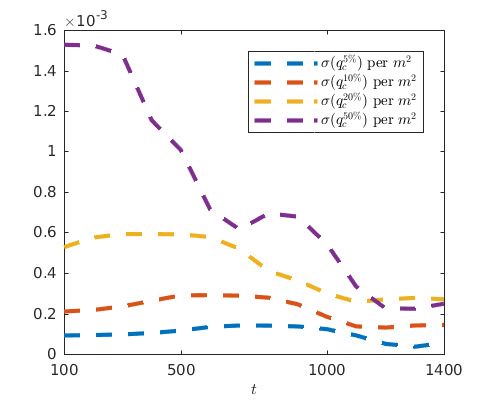
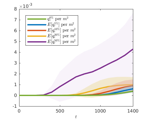
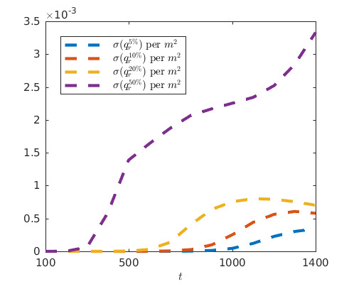
Figure 20. Example 7: Time evolution of the expected values with their standard deviations for the cloud variables per $m^{2}$ (shaded region, left column) and standard deviation (right column) for $\nu=0.05$, $0.1$, $0.2$ and $0.5$ (from top to down).

These averaged quantities show the qualitative difference in the different perturbations scenarios, as already described above. For low perturbations, the difference of the expectation value is quite small and also the standard deviation remains small. For increasing perturbations, the spread is increased. As noted before, the averaged quantities are dominated by the positive perturbations, leading to (i) earlier cloud formation, (ii) thicker clouds due to more available water vapor, and (iii) to enhanced rain formation. These three features can be seen very nicely in the strongest perturbations ($\nu=0.5$), with a large drop in water vapor concentration accompanied by a strong increase in cloud water and earlier onset of precipitation. We would also like to note that the spread is only given by the standard deviation, whereas the actual minima (for instance, almost no cloud formation) cannot be seen directly, although these scenarios are possible.

Example 8: 2-D case with stochastic parameters

In the following experiment we study uncertainty propagation due to incomplete information about the model parameters which is a very typical problem arising in atmospheric science. We chose the same initial data for the flow and cloud variables as in Section 4.2. More precisely, we take the following initial cloud variables:

$$(\widehat{q_{v}})_{0}(\bm{x},0)=0.02\theta^{\prime}(\bm{x},0),\quad(\widehat{q_{v}})_{k}(\bm{x},0)=(\widehat{q_{c}})_{k}(\bm{x},0)=(\widehat{q_{r}})_{k}(\bm{x},0)=0\quad\mbox{for}\quad 1\leq k\leq M.$$

Consequently, in order to investigate uncertainty propagation in the numerical solution we choose $10\%$, $20\%$ and $50\%$ perturbation of these coefficients, namely, we take

$$(\widehat{k_{1}})_{0} =0.0041,\quad(\widehat{k_{1}})_{1}=\nu(\widehat{k_{1}})_{0},\quad(\widehat{k_{1}})_{k}=0\quad\mbox{for}\quad 2\leq k\leq M,$$

$$(\widehat{k_{2}})_{0} =0.8,\quad(\widehat{k_{2}})_{1}=\nu(\widehat{k_{2}})_{0},\quad(\widehat{k_{2}})_{k}=0\quad\mbox{for}\quad 2\leq k\leq M,$$

$$\widehat{\alpha}_{0} =190.3,\quad\widehat{\alpha}_{1}=\nu\widehat{\alpha}_{0},\quad\widehat{\alpha}_{k}=0\quad\mbox{for}\quad 2\leq k\leq M,$$

where $\nu=0.1$, 0.2 and 0.5, respectively. The numerical solution is computed at time $t=1400s$ on a $320\times 320$ mesh. Figures 21 and 22 present the potential temperature $\theta$ and the expected values of the cloud drops concentration $q_{c}$, respectively, for $\nu=0$, $0.1$, $0.2$ and $0.5$.

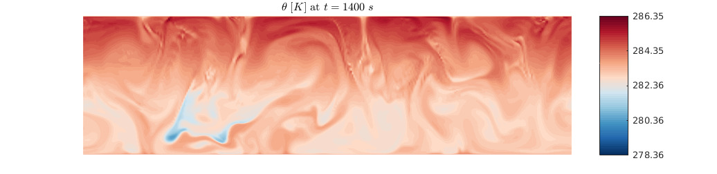
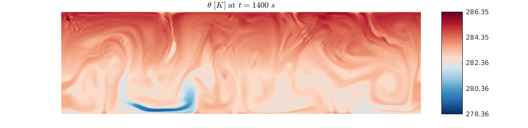
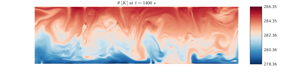
Figure 21. Example 8: Potential temperature $\theta$ for $\nu=0$, $0.1$, $0.2$ and $0.5$ (from top to down).

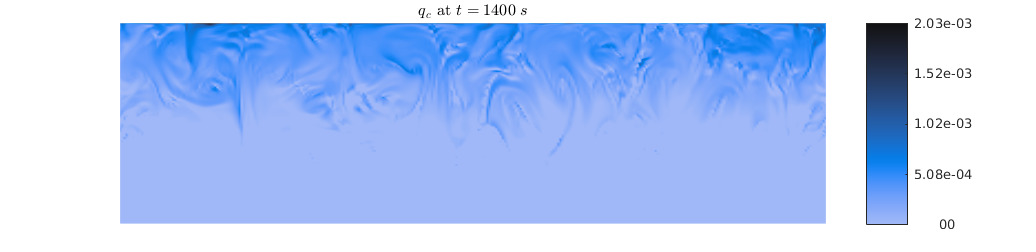
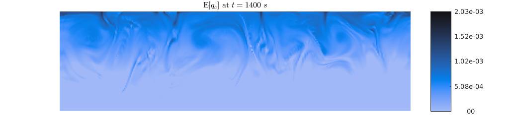
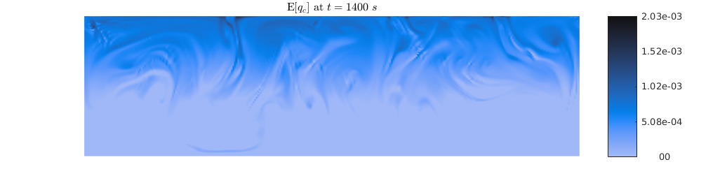
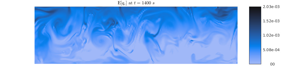
Figure 22. Example 8: Cloud drops concentration $q_{c}$ for $\nu=0$, $0.1$, $0.2$ and $0.5$ (from top to down).

In these scenarios with perturbed cloud model parameters, the overall structures are more stable and changes are less pronounced than in Example 7. Nevertheless, the main features of the variations are obviously driven by precipitation processes since the only perturbed parameters are those determining rain processes. Again, one key feature of the perturbed scenarios is the signature of evaporating rain in lower levels of the 2-D domain. For positive perturbations, that is, larger parameters $k_{1}$, $k_{2}$ and $\alpha$, rain formation is enhanced (more rain is formed from cloud water, due to larger $k_{1}$ and $k_{2}$) and sedimentation is enhanced (more rain is falling downwards due to larger $\alpha$). Thus, more rain water is transported downwards into subsaturated regions, which is then evaporated inducing cooling due to latent heat consumption. These positive variations again dominate the potential temperature field; see Figure 21. For the cloud water field (Figure 22), one can observe higher expected values for stronger perturbations. This is probably due to the fact that more rain is evaporated in lower levels, thus more water vapor is then available for cloud formation in upward motions of the convective cells. This redistribution of water vapor as well as the reduction of rain for negative perturbation lead to larger variations of cloud water in the 2-D domain, as can be seen in the standard deviation for the cloud drops concentration $q_{c}$, as depicted in Figure 23.

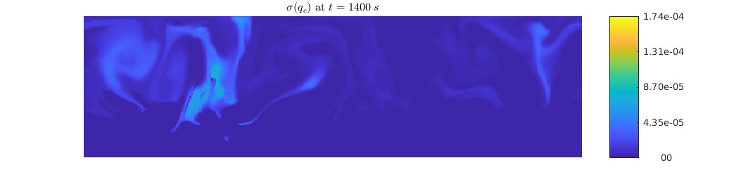
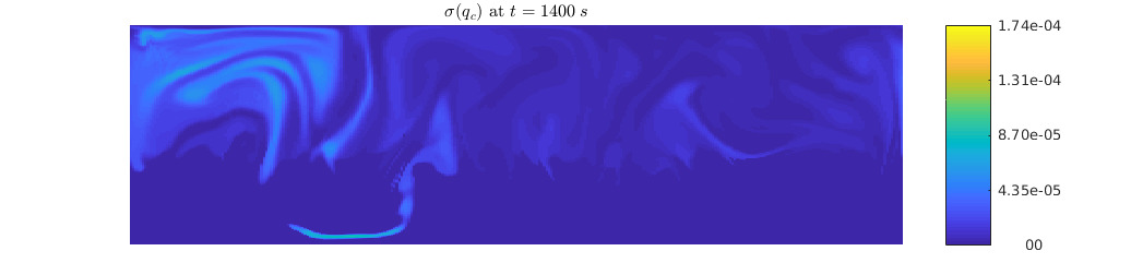
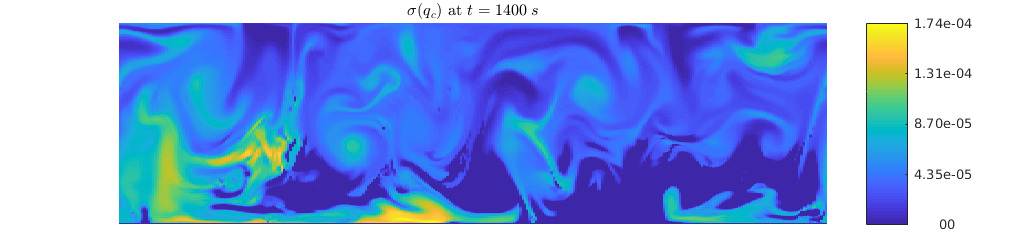
Figure 23. Example 8: Standard deviation of the cloud drops concentration $q_{c}$ for $\nu=0.1$, $0.2$ and $0.5$ (from top to down).

The expected values as well as the standard deviation for the cloud variables vary considerably with respect to the perturbation of model parameters; see Figure 24. Our numerical experiments indicate that the standard deviation increases in time and also depends on the size of the parameter perturbation. Indeed, the larger the parameter perturbation, the higher is the standard deviation of the cloud variables. The size of the corresponding standard deviations is depicted in the right column of Figure 24. As expected, rain formation sets on earlier for large perturbations, leading also to a strong decrease in the overall water vapor in comparison to less perturbed scenarios. However, the variations in all water variables increase a lot from the onset of precipitation to later times, and even the spread in cloud water increases in contrast to the time evolution in Example 7. Generally, the spread in the mean values is smaller than in Example 7; changes in initial data produce a larger variation, that means the model physics is quite stable with respect to perturbations in rain process formulations.

        

        

        

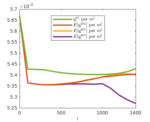
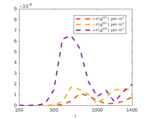
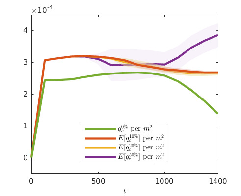
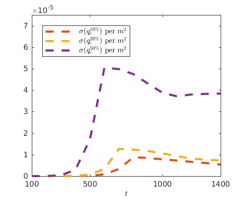
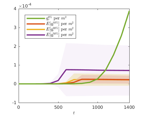
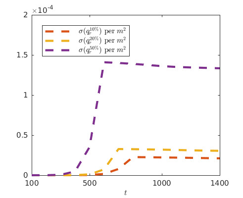
Figure 24. Example 8: Time evolution of the expected values with their standard deviations for the cloud variables per $m^{2}$ (shaded region, left column) and standard deviation (right column) for $\nu=0.1$, $0.2$ and $0.5$ (from top to down).

Example 9: 3-D case with stochastic initial data

Similarly to Example 7, we now investigate the uncertainty quantification in the 3-D Rayleigh-Bénard convection for stochastically perturbed initial data of the cloud variables given by (7.1). The numerical solution is computed in a domain $\Omega=[0,5000]\times[0,5000]\times[0,1000]\,\mathrm{m^{3}}$, which is discretized using $50\times 50\times 50$ mesh cells. In Figure 25, we show the influence of $0\%$, $10\%$, $20\%$ and $50\%$ perturbation on the potential temperature $\theta$ as well as the expected value of the cloud drop concentration $q_{c}$. For the perturbation scenarios in the case of the 3-D moist Rayleigh-Bénard convection, one can see overall a qualitatively similar picture as for the corresponding 2-D simulations. However, due to an additional spatial direction, the 3-D structures can further change their patterns. For positive perturbations, clouds can be formed even at low vertical upward motions. The latent heat release increases the vertical motions in the convective cells, which leads to additional feedback, such as stronger cloud formation, which in turn leads to formation of larger amount of rain water. As in the 2-D case, the potential temperature distribution changes considerably at lower levels of the 3-D domain since evaporative cooling of precipitation is a dominant process. Similarly, the mean cloud water distribution is crucially changed. For positive perturbations, which are dominant on average in the beginning, more cloud water is formed and is later removed. Thus, less cloud water is available in the domain at later times. This can also be seen in the time evolution of spatially averaged variables, as shown in Figure 26, where the time evolution of the mean expected value per $m^{3}$ and the mean standard deviation per $m^{3}$ of the cloud variables are plotted. The time evolution of these variables is very similar to the 2-D case, but the 3-D scenarios show a very interesting feature, which is not available in 2-D. For larger perturbations, the pattern of the convective cells is changed. While convective cells have a quasi hexagonal shape for the deterministic simulation, they are ordered in a different way for larger perturbations. At upper levels, a more roll-like structure or even rectangular shape is formed. Thus, there is a transition of structures due to perturbations in the initial conditions. This feature has not been documented until now. A more detailed analysis of these structures is left for future studies.

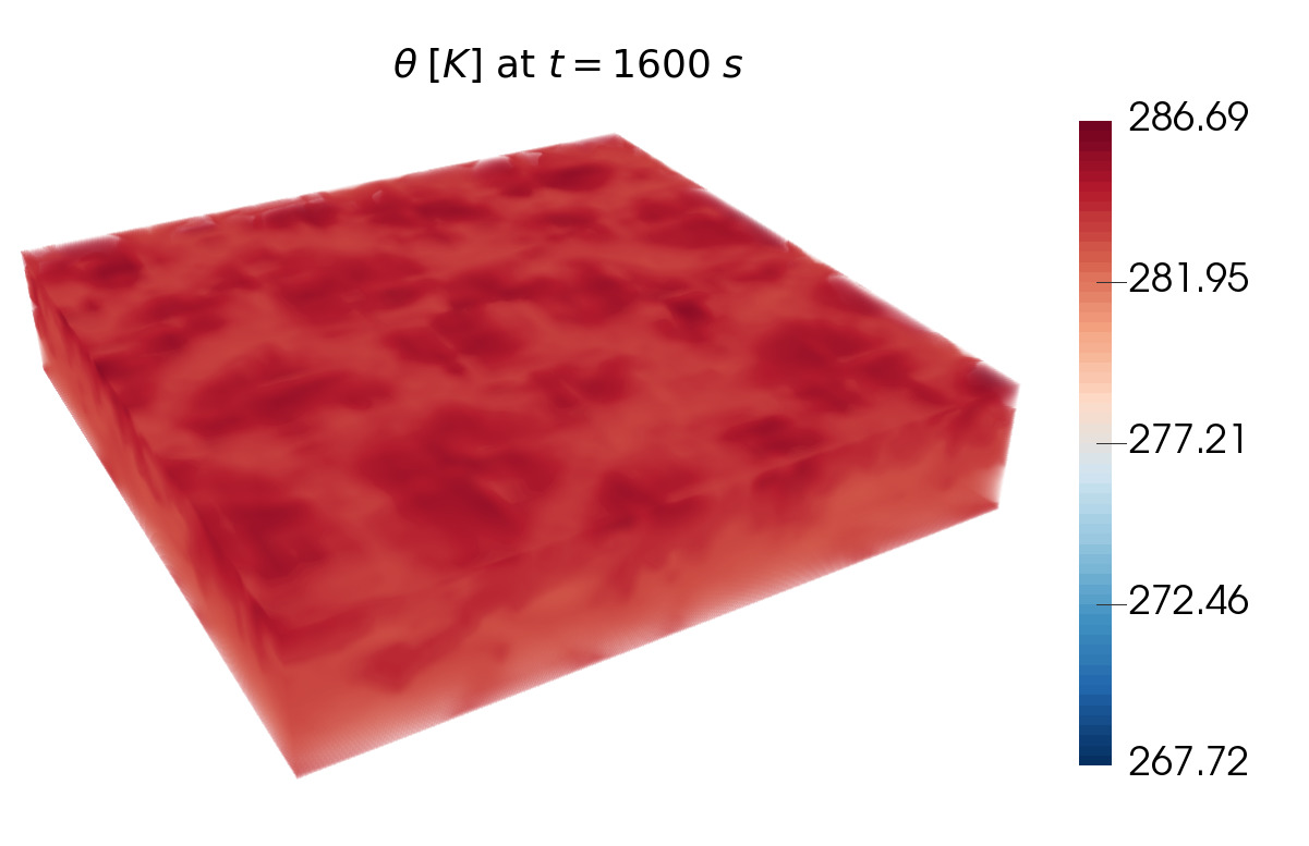
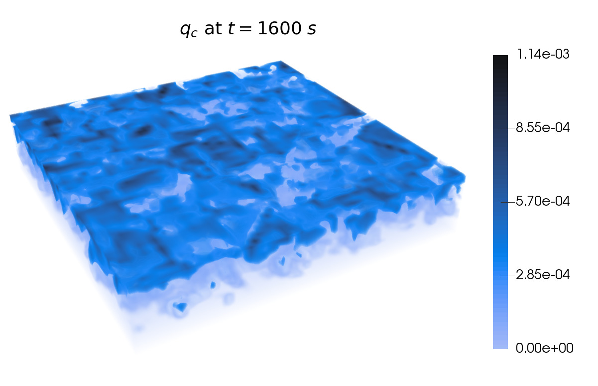
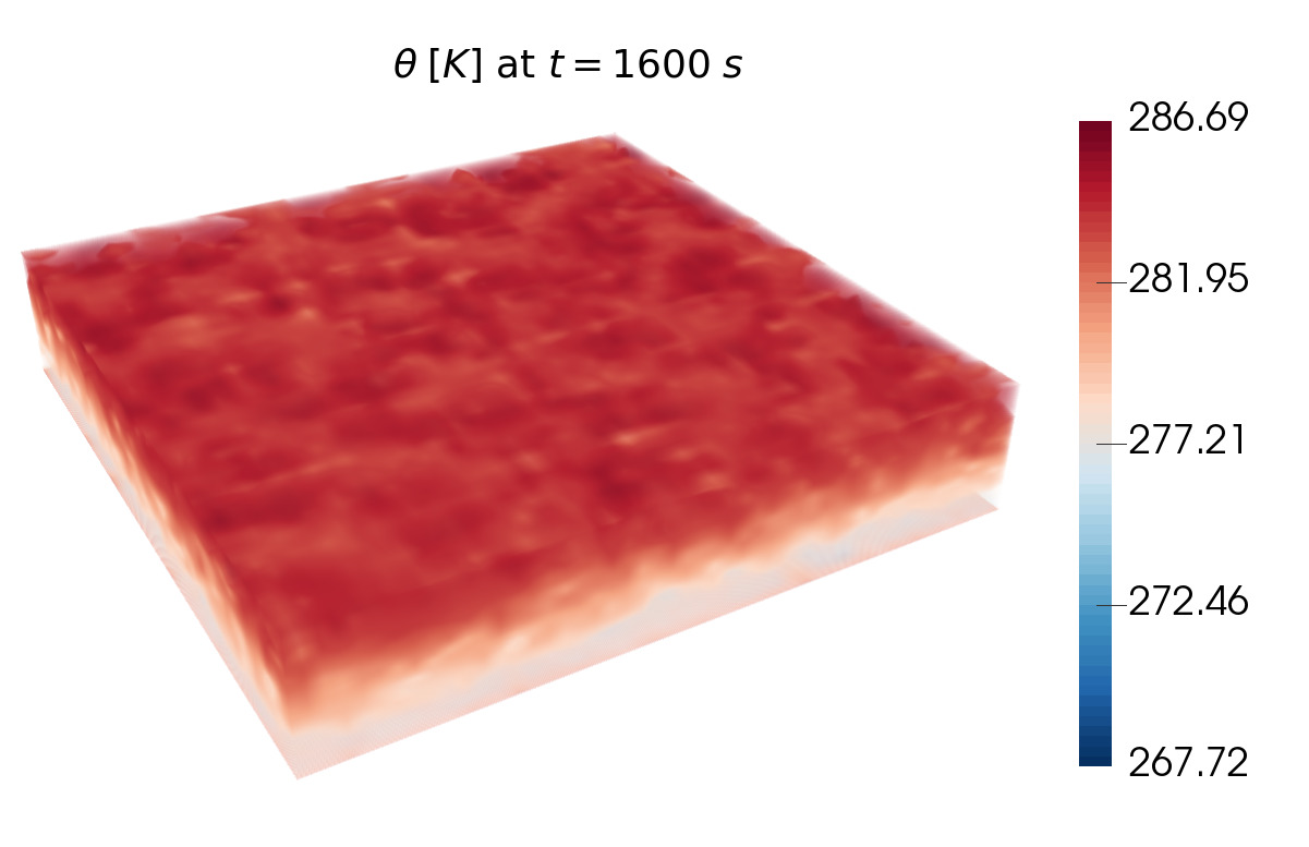
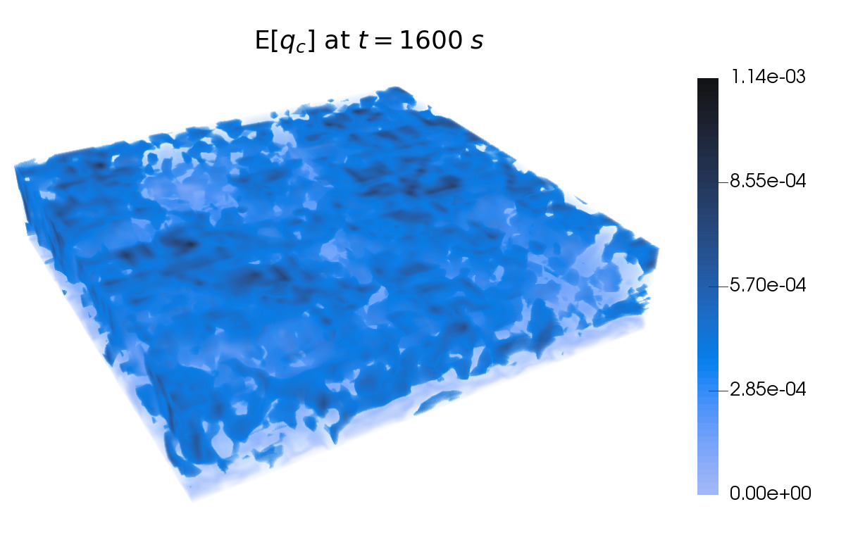
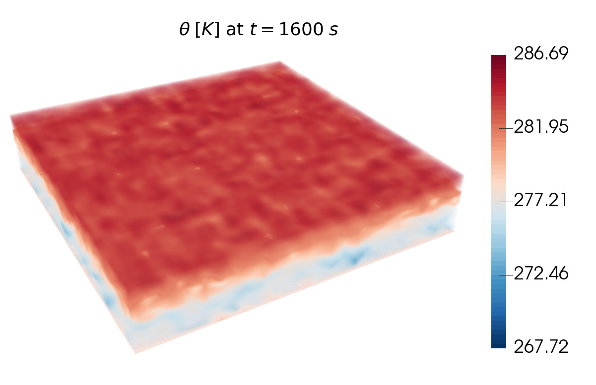
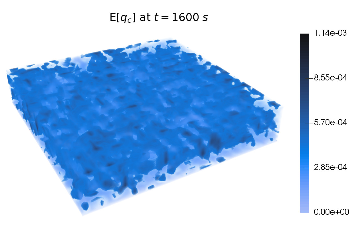
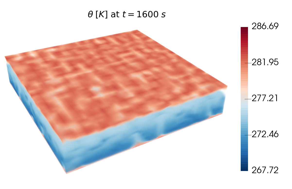
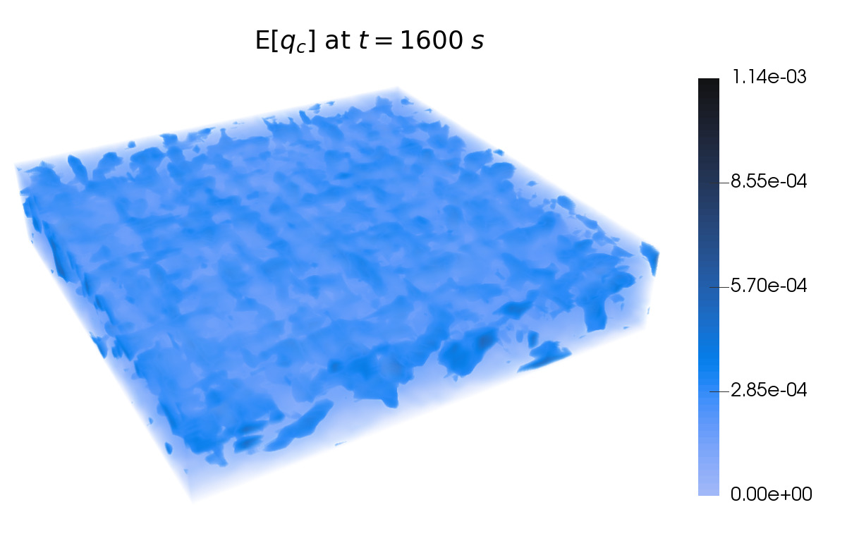
Figure 25. Example 9: Potential temperature $\theta$ (left column) and cloud drops concentration $q_{c}$ (right column) using $0\%$, $10\%$, $20\%$ and $50\%$ (from top to down) perturbation of the initial data in $q_{v}$.

        

        

        

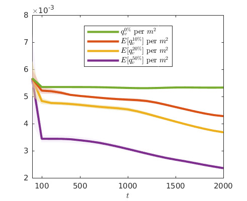
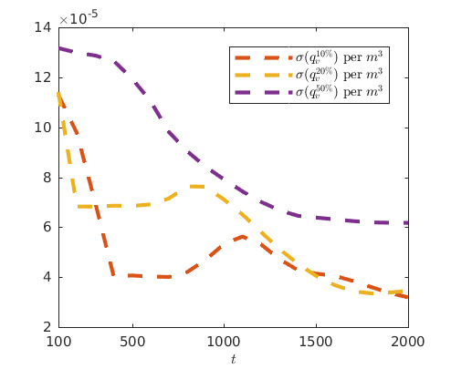
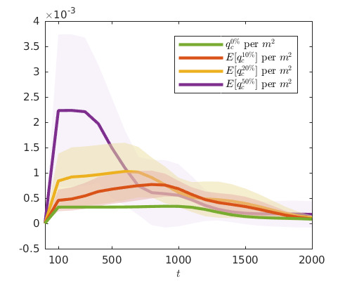
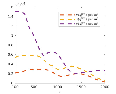
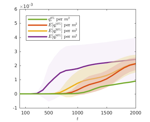
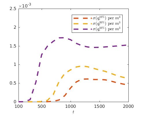
Figure 26. Example 9: Time evolution of the expected values with their standard deviations for the cloud variables per $m^{3}$ (shaded region, left column) and standard deviation (right column) using $0\%$, $10\%$, $20\%$ and $50\%$ (from top to down) perturbation of the initial data in $q_{v}$.

8. Conclusion

In the present paper, we have studied uncertainty propagation in an atmospheric model that combines the Navier-Stokes equations for weakly compressible fluids (2) with the cloud equations (2). The latter has been recently proposed in [34] and is based on the so-called single moment approach considering the evolution equations for the mass concentrations of the water vapor, cloud drops and rain. Our numerical strategy is based on the stochastic Galerkin method that combines a finite-volume method for space-time discretization with a spectral approximation in the stochastic space. We point out that atmospheric flows are weakly compressible which leads to the low Mach number problem. One therefore needs to use a finite-volume method, which is accurate and efficient in the low Mach number regime; see [6, 5]. To this end, we have chosen a suitable linear-nonlinear splitting between the fast and slow flow variables and the second-order IMEX discretization in time (the ARS (2,2,2) scheme) as described in Section 3. Coupling between the cloud model (2) and the Navier-Stokes system (2.2) is realized numerically by the second-order Strang splitting. The cloud equations are approximated in space by the finite-volume method and in time using the explicit third-order Runge-Kutta method with an enlarged stability region as explained in Section 3. Note that microscopic cloud dynamics requires a smaller time step than the flow dynamics and thus several microscopic cloud subiterations are realized within one macroscopic splitting time step, whose size is dictated by the flow dynamics. To the best of our knowledge, this is the first contribution that combines an accurate and efficient method for the weakly compressible Navier-Stokes equations with the stochastic Galerkin method for the uncertainty quantification of time evolution of the mass densities of water vapor, cloud drops and rain.

We have conducted extensive numerical benchmarking for both the deterministic and stochastic models and present the obtained numerical results in Sections 4 and 7. In the latter, we took into account the uncertainties in both initial data and cloud model parameters. Our numerical study clearly demonstrates applicability of the stochastic Galerkin method for the uncertainty quantification in complex atmospheric models. We have obtained interesting results illustrating the behavior of clouds in different perturbed scenarios and demonstrated that perturbations in the initial conditions can crucially change the time evolution of the moist Rayleigh-Bénard convection. In particular, it has been shown that for larger perturbation, on average the positive perturbations dominate the expectation values, although the standard deviation can be quite large. The main feature is a strong evaporative cooling in lower levels of the (2-D/3-D) domain due to enhance rain formation and sedimentation into low humidity levels. In the 3-D case, a change in the formed pattern can be seen, changing from hexagons to rolls/rectangles, which is quite surprising. For perturbations in parameters for rain processes, the results are also dominated by the positive part of the perturbations. Since rain processes are affected, the spread in the time evolution is increasing since the changes depend crucially on the interaction of formed rain drops with other variables. Overall, it seems that for cloud physics, the expectation values are dominated by the positive perturbations leading to a change in the distributions. This is an interesting topic for detailed studies in future. Our further goal is to extend the developed numerical method to the fully random Navier-Stokes-cloud system by considering random weakly compressible Navier-Stokes equations. We are also interested in considering different random effects, such as initial data, boundary data and model parameters simultaneously, which would require a multivariate stochastic Galerkin method. This will allow one to quantify more precisely the propagation of small scale stochastic errors initiated at cloud scales to macroscopic scales of flow dynamics.

Acknowledgement
The research leading to these results has been done within the sub-project A2 of the Transregional Collaborative Research Center SFB/TRR 165 “Waves to Weather” funded by the German Science Foundation (DFG). The work of A. Chertock was supported in part by NSF grants DMS-1521051 and DMS-1818684. The work of A. Kurganov was supported in part by NSFC grant 11771201 and NSF grants DMS-1521009 and DMS-1818666.

The authors gratefully acknowledge the support of the Data Center (ZDV) in Mainz for providing computation time on MOGON and MOGON II clusters and of NSF RNMS Grant DMS-1107444 (KI-Net). M. Lukáčová-Medvid’ová and B. Wiebe would like to thank L. Yelash (University of Mainz) for fruitful discussions. P. Spichtinger would like to thank P. Reutter (University of Mainz) for fruitful discussions on the results of the 2-D/3-D simulations.

9. Appendix A: Closure for single moment schemes

The number concentration of rain drops can be approximated by a function of the respective mass concentration $n_{r}=f(q_{r},c_{r})$. Since we implicitly assume that rain drops are distributed according to a size distribution, this approach should be used for mimicking the shape of the distribution in a proper way. If we use a constant mean mass of rain drops, the function will be a simple linear relation $n_{r}=\frac{1}{\overline{m}_{r}}q_{r}$. We extend this approach and propose the following nonlinear relation:

$$n_{r}=c_{r}\cdot q_{r}^{\gamma},\quad 0<\gamma\leq 1.$$

Using this approach, one can replace the quantity $n_{r}$ in the processes related to rain drop number concentration. For the simple case of a constant mean mass $\overline{m}_{r}$, we can determine the constants as $c_{r}=\overline{m}_{r}^{-1}$ and $\gamma=1$. This approach would be meaningful for the case of a symmetric size distribution of rain droplets centered around the mean mass. However, it is well-known that size distributions of rain are usually skew to larger sizes and thus a linear relation is inappropriate. For sizes of rain drops, an exponential distribution is often assumed (see [25]), namely:

$$f(r)=B_{r}e^{-\lambda r}$$

with a constant parameter $B_{r}=2\cdot 10^{7}\,\mathrm{m}^{-4}$ and the drop radius $r$. Using the general moments of the distribution,

$$\mu_{k}[r]=\frac{\Gamma(k+1)}{\lambda^{k+1}}B_{r}$$

with the gamma function $\Gamma(x):=\int_{0}^{\infty}t^{x-1}\exp(-t)\,dt$, we obtain

$$\rho n_{r}=\mu_{0}[r]=\frac{B_{r}}{\lambda}\quad\mbox{and}\quad\rho q_{r}=\frac{4}{3}\pi\rho_{\ell}\frac{\Gamma(4)}{\lambda^{4}}B_{r}.$$

Using these relations, one can derive the following function for the number concentration $n_{r}$:

$$n_{r}=\underbrace{B_{r}^{\frac{3}{4}}\rho^{-\frac{3}{4}}\left(8\pi\rho_{\ell}\right)^{-\frac{1}{4}}}_{=c_{r}}q_{r}^{\frac{1}{4}}=c_{r}q_{r}^{\gamma},\quad\gamma=\frac{1}{4}.$$

We stress that $c_{r}$ is, in fact, a function of the air density $\rho$, that is, $c_{r}=c_{r0}\cdot\rho^{-\frac{3}{4}}$.

10. Appendix B: Explicit formulation of the cloud equations

We present the equations of microphysical processes in an explicit way as they are used in our numerical experiments. In Tables 3 and 4, we present physical constants and model parameters with their values used in our numerical simulations.

$$n_{c} =q_{c}\frac{8\cdot 10^{8}}{q_{c}+4.1888\cdot 10^{-7}}\coth\left(\frac{q_{c}}{5.236\cdot 10^{-13}}\right),\quad C_{{\rm act}}=6.2832\cdot 10^{-3}D_{v}G\rho\left(q_{v}-q_{*}\right)_{+},$$

$$C_{1} =0.7796D_{v}G\left(q_{v}-q_{*}\right)\left(\frac{8\cdot 10^{8}}{q_{c}+4.1888\cdot 10^{-7}}\coth\left(\frac{q_{c}}{5.236\cdot 10^{-13}}\right)\right)^{\frac{2}{3}}\rho q_{c},$$

$$p_{s}(T) =\exp\Big{\{}54.842763-\nicefrac{{6763.22}}{{T}}-4.21\ln T+0.000367T+\tanh(0.0415(T-218.8))$$

$$\quad\cdot(53.878-\nicefrac{{1331.22}}{{T}}-9.44523\ln T+0.014025T)\Big{\}},$$

$$n_{r} =23752.6753\rho^{-\frac{3}{4}}q_{r}^{\frac{1}{4}},\quad r=\left(\frac{1.21\cdot 10^{-5}}{q_{r}+0.2874\rho^{-\frac{3}{4}}q_{r}^{\frac{1}{4}}}\right)^{\frac{4}{15}},$$

$$E =-0.7796D_{v}G\left(q_{*}-q_{v}\right)_{+}\left(644.5198\sqrt{\rho q_{r}}+17.5904\mu^{-\frac{1}{6}}D_{v}^{-\frac{1}{3}}\sqrt{\alpha r}\rho^{\frac{13}{24}}q_{r}^{\frac{91}{120}}\right),$$

$$A_{1} =10^{-3}k_{1}\rho q_{c}^{2},\quad A_{2}=0.3846\alpha k_{2}\rho^{\frac{1}{4}}q_{c}rq_{r}^{\frac{61}{60}},\quad v_{q}=1.1068\alpha q_{r}^{\frac{4}{15}}r\rho^{-\frac{1}{2}}.$$

Constant	Description
$p_{*}=$101\,325\text{\,}\mathrm{Pa}$$	reference pressure
$T_{*}=$288\text{\,}\mathrm{K}$$	reference temperature
$T_{0}=$273.15\text{\,}\mathrm{K}$$	melting temperature
$\rho_{*}=$1.225\text{\,}\mathrm{kg}\text{\,}{\mathrm{m}}^{-3}$$	reference air density
$\rho_{l}=$1000\text{\,}\mathrm{kg}\text{\,}{\mathrm{m}}^{-3}$$	density of liquid water
$R_{v}=$461.52\text{\,}\mathrm{J}\text{\,}{\mathrm{kg}}^{-1}\text{\,}{\mathrm{K}}^{-1}$$	specific gas constant, water vapor
$c_{p}=$1005\text{\,}\mathrm{J}\text{\,}{\mathrm{kg}}^{-1}\text{\,}{\mathrm{K}}^{-1}$$	specific heat capacity, dry air
$g=$9.81\text{\,}\mathrm{m}\text{\,}{\mathrm{s}}^{-2}$$	acceleration due to gravity
$L=$2.53\text{\times}{10}^{6}\text{\,}\mathrm{J}\text{\,}{\mathrm{kg}}^{-1}$$	latent heat of vaporization
$\varepsilon=\frac{M_{\text{mol},v}}{M_{\text{mol},a}}=0.622$	ratio of molar masses of water and dry air
$D_{0}=$2.11\text{\times}{10}^{-5}\text{\,}{\mathrm{m}}^{2}\text{\,}{\mathrm{s}}^{-1}$$	diffusivity constant

Table 3. Physical constants and reference quantities, [34].

Parameter	Description
$\alpha=190.3\pm 0.5\cdot$190.3\text{\,}\mathrm{m}\text{\,}{\mathrm{s}}^{-1}\text{\,}{\mathrm{kg}}^{-\beta}$$	parameter for terminal velocity
$k_{1}=0.0041\pm 0.5\cdot$0.0041\text{\,}\mathrm{kg}\text{\,}{\mathrm{s}}^{-1}$$	parameter for autoconversion
$k_{2}=0.8\pm 0.5\cdot$0.8\text{\,}\mathrm{kg}$$	parameter for accretion
$\beta=\frac{4}{15}$	parameter for terminal velocity
$m_{t}=$1.21\text{\times}{10}^{-5}\text{\,}\mathrm{kg}$$	parameter for terminal velocity
$N_{0}=$1000\text{\,}{\mathrm{m}}^{-3}$$	parameter for activation
$N_{\infty}=$8\text{\times}{10}^{8}\text{\,}{\mathrm{kg}}^{-1}$$	parameter for activation
$m_{0}=$5.236\text{\times}{10}^{-16}\text{\,}\mathrm{kg}$$	parameter for activation
$a_{E}=0.78$	parameter for evaporation
$a_{v}=0.78$	parameter for ventilation
$b_{v}=0.308$	parameter for ventilation

Table 4. Model parameters, [34].

References

- [1] T. Alboussière and Y. Ricard. Rayleigh-Bénard stability and the validity of quasi-Boussinesq or quasi-anelastic liquid approximations. J. Fluid Mech., 817:264–305, 2017.
- [2] U. M. Ascher, S. J. Ruuth, and R. J. Spiteri. Implicit-explicit Runge-Kutta methods for time-dependent partial differential equations. Appl. Numer. Math., 25(2-3):151–167, 1997. Special issue on time integration (Amsterdam, 1996).
- [3] M. Baldauf, J. Förstner, S. Klink, T. Reinhardt, C. Schraff, A. Seifert, and K. Stephan. Kurze modell- und datenbankbeschreibung COSMO-DE (LMK). 2014.
- [4] K. D. Beheng. The Evolution of Raindrop Spectra: A Review of Microphysical Essentials. In F. Y. Testik and M. Gebremichael, editors, Rainfall: State of the Science, Geophysical Monograph Series, pages 29–48, 2010.
- [5] G. Bispen. IMEX finite volume schemes for the shallow water equations, PhD thesis. Johannes Gutenberg-University, Mainz, 2015.
- [6] G. Bispen, M. Lukáčová-Medvid’ová, and L. Yelash. Asymptotic preserving IMEX finite volume schemes for low Mach number Euler equations with gravitation. J. Comput. Phys., 2017.
- [7] G. H. Bryan and J. M. Fritsch. A benchmark simulation for moist nonhydrostatic numerical models. Mont. Weather Rev., 130:2917–2928, 2002.
- [8] C. Canuto. Spectral Methods - Fundamentals in Single Domains. Springer, 2006.
- [9] R. M. Davies and F. J. Taylor. The mechanism of large bubbles rising through extended liquids and through liquids in tubes. Proc. Royal Soc. Lond. A, 200:375–390, 1950.
- [10] B. Després, G. Poëtte, and D. Lucor. Robust uncertainty propagation in systems of conservation laws with the entropy closure method. In Uncertainty Quantification in Computational Fluid Dynamics, pages 105–149. Springer, 2013.
- [11] J. Dixon. The Shock Absorber Handbook. Wiley, 2007.
- [12] H. C. Elman, C. W. Miller, E. T. Phipps, and R. S. Tuminaro. Assessment of collocation and Galerkin approaches to linear diffusion equations with random data. Int. J. Uncertain. Quantif., 1(1):19–33, 2011.
- [13] A. V. Getling. Rayleigh-Bénard convection, Structure and Dynamics. World Sci. Publ., Singpore, 2001.
- [14] W. W. Grabowski. Untangling microphysical impacts on deep convection applying a novel modeling methodology. J. Atmos. Sci., 72(6):2446–2464, 2015.
- [15] A. L. Igel and S. C. van den Heever. The role of latent heating in warm frontogenesis. Quart. J. Roy. Met. Soc., 140(678, A):139–150, 2014.
- [16] E. Kessler. On the distribution and continuity of water substance in atmospheric circulations., volume 32 of Meteorol. Monographs. American Meteorological Society, Boston, 1969.
- [17] A. P. Khain, M. Ovtchinnikov, M. Pinsky, A. Pokrovsky, and H. Krugliak. Notes on the state-of-the-art numerical modeling of cloud microphysics. Atmos. Res., 55(3-4):159 – 224, 2000.
- [18] V. I. Khvorostyanov. Mesoscale processes of cloud formation, cloud-radiation interaction, and their modeling with explicit cloud microphysics. Atmos. Res., 39(1-3):1–67, 1995.
- [19] H. Köhler. The nucleus in and the growth of hygroscopic droplets. T. Faraday Soc., 32(2):1152–1161, 1936.
- [20] A. Kurganov. Finite-volume schemes for shallow-water equations. Acta Numer., 27:289–351, 2018.
- [21] D. Lamb and J. Verlinde. Physics and chemistry of clouds. Cambridge University Press, 2011.
- [22] M. Lukáčová-Medvid’ová, J. Rosemeier, P. Spichtinger, and B. Wiebe. IMEX finite volume methods for cloud simulation. In Finite volumes for complex applications VIII—hyperbolic, elliptic and parabolic problems, volume 200 of Springer Proc. Math. Stat., pages 179–187. Springer, Cham, 2017.
- [23] X. Ma and N. Zabaras. An adaptive hierarchical sparse grid collocation algorithm for the solution of stochastic differential equations. J. Comput. Phys., 228(8):3084–3113, 2009.
- [24] P. J. Marinescu, S. C. van den Heever, S. M. Saleeby, S. M. Kreidenweis, and P. J. DeMott. The microphysical roles of lower-tropospheric versus midtropospheric aerosol particles in mature-stage mcs precipitation. J. Atmos. Sci., 74(11):3657–3678, 2017.
- [25] J. S. Marshall and W. McK. Palmer. The distributions of raindrops with size. J. Meteorol., 5:165–166, 1948.
- [26] A. A. Medovikov. Dumka 3 code, available at http://dumkaland.org/.
- [27] A. A. Medovikov. High order explicit methods for parabolic equations. BIT, 38(2):372–390, 1998.
- [28] S. Mishra and C. Schwab. Sparse tensor multi-level Monte Carlo finite volume methods for hyperbolic conservation laws with random initial data. Math. Comp., 81(280):1979–2018, 2012.
- [29] S. Mishra, C. Schwab, and J. Šukys. Multi-level Monte Carlo finite volume methods for uncertainty quantification in nonlinear systems of balance laws. In Uncertainty quantification in computational fluid dynamics, volume 92 of Lect. Notes Comput. Sci. Eng., pages 225–294. Springer, Heidelberg, 2013.
- [30] D. Murphy and T. Koop. Review of the vapour pressure of ice and supercooled water for atmospheric applications. Quarterly Journal of the Royal Meterorological Society, 131:1539–1565, 2005.
- [31] O. Pauluis and J. Schumacher. Idealized moist Rayleigh-Bénard convection with piecewise linear equation of state. Comm. Math. Sci., 8:295–319, 2010.
- [32] M. D. Petters and S. M. Kreidenweis. A single parameter representation of hygroscopic growth and cloud condensation nucleus activity. Atmos. Chem. Phys., 7(8):1961–1971, 2007.
- [33] G. Poëtte, B. Després, and D. Lucor. Uncertainty quantification for systems of conservation laws. J. Comput. Phys., 228(7):2443–2467, 2009.
- [34] N. Porz, M. Hanke, M. Baumgartner, and P. Spichtinger. A consistent model for liquid clouds. Math. Clim. Weather Forecast., 4(1):50–78, 2018.
- [35] H. R. Pruppacher and J. D. Klett. Microphysics of Clouds and Precipitation. Springer, 2010.
- [36] D. Schuster, S. Brdar, M. Baldauf, A. Dedner, R. Klöfkorn, and D. Kröner. On discontinuous Galerkin approach for atmospheric flow in the mesoscale with and without moisture. Meteorol. Z., 23(4):449–464, 2011.
- [37] J. Šukys, S. Mishra, and C. Schwab. Multi-level Monte Carlo finite difference and finite volume methods for stochastic linear hyperbolic systems. In Monte Carlo and quasi-Monte Carlo methods 2012, volume 65 of Springer Proc. Math. Stat., pages 649–666. Springer, Heidelberg, 2013.
- [38] M. Szakall, K. Diehl, S. K. Mitra, and S. Borrmann. A wind tunnel study on the shape, oscillation, and internal circulation of large raindrops with sizes between 2.5 and 7.5 mm. Journalof the Atmospheric Sciences, 66(3):755–765, 2009.
- [39] M. Szakall, S. K. Mitra, K. Diehl, and S. Borrmann. Shapes and oscillations of falling raindrops - a review. Atmospheric Research, 97(4, SI):416–425, 2010.
- [40] J. Tryoen, O. Le Maître, M. Ndjinga, and A. Ern. Intrusive Galerkin methods with upwinding for uncertain nonlinear hyperbolic systems. J. Comput. Phys., 229(18):6485–6511, 2010.
- [41] X. Wan and G. E. Karniadakis. Long-term behavior of polynomial chaos in stochastic flow simulations. Comput. Methods Appl. Mech. Engrg., 195(41-43):5582–5596, 2006.
- [42] J. Warner. The microstructure of cumulus cloud. part i. general features of the droplet spectrum. J. Atmos. Sci., 26(5):1049–1059, 1969.
- [43] T. Weidauer and J. Schumacher. Toward a mode reduction strategy in shallow moist convection. New Journal of Physics, 15:125025–125249, 2013.
- [44] J. A. S. Witteveen, A. Loeven, and H. Bijl. An adaptive stochastic finite elements approach based on Newton-Cotes quadrature in simplex elements. Comput. & Fluids, 38(6):1270–1288, 2009.
- [45] D. Xiu and J. S. Hesthaven. High-order collocation methods for differential equations with random inputs. SIAM J. Sci. Comput., 27(3):1118–1139 (electronic), 2005.
- [46] D. Xiu and G. E. Karniadakis. The Wiener-Askey polynomial chaos for stochastic differential equations. SIAM J. Sci. Comput., 24(2):619–644 (electronic), 2002.