Adversarial Examples as
an Input-Fault Tolerance Problem

Abstract

We analyze the adversarial examples problem in terms of a model’s fault tolerance with respect to its input. Whereas previous work focuses on arbitrarily strict threat models, i.e., $\epsilon$-perturbations, we consider arbitrary valid inputs and propose an information-based characteristic for evaluating tolerance to diverse input faults.

1 Introduction

Fault tolerance is a qualitative term that refers to the ability of a system to perform within specification despite faults in its subsystems. A way of characterizing a complex system’s fault tolerance is to measure its performance under induced faults of varying strength. In particular for systems operating in safety-critical settings [21], it is desirable that the performance degrades gradually as a function of fault severity and consistently so across a variety of fault types.

Most of the literature on the fault tolerance of artificial neural networks considers internal faults, such as deliberate [12, 29] or accidental [25, 20, 31] neuron outage. Modern deep networks, however, are presented with increasingly complex data, and many applications demand predictable performance for all inputs, e.g., low-confidence outputs for out-of-distribution inputs. Therefore, characterizing the fault tolerance of the overall system requires considering the input itself as a source of external faults [5, 34]. We suggest that the adversarial examples phenomenon, which exposes unstable model behaviour for valid bounded inputs [30, 16, 19, 4, 2, 1], be interpreted as a type of external fault.

As a measure of a model’s tolerance to adversarial attacks of increasing strength, we propose the information conveyed about the target variable, i.e., the label in a classification task [26, 32]. We find this measure to be more representative of a model’s expected robustness than a previous convention of reporting the test error rate for fixed $\epsilon$-perturbations. The proposed characteristic curves reduce the need for human supervision to distinguish mistakes from ambiguous instances [28, 3], which is subjective and time consuming.

We expose a convolutional network to a range of different attacks and observe that: i) the proposed robustness measure is sensitive to hyper-parameters such as weight decay, ii) prediction accuracies may be identical, while the information curves differ, and iii) more gradual changes in the information conveyed by the model prediction corresponds to improved adversarial robustness.

2 Methodology

We introduce a way of quantifying input-fault tolerance for arbitrary inputs in terms of the mutual information (MI), $I(T;Y)$, between a model’s categorical prediction and the true label, represented by the random variables that $T$ and $Y$, respectively. The MI can be written as $I(T;Y)=H(Y)-H(Y|T)$, where $H$ denotes the Shannon entropy in bits, which is a measure of uncertainty. Perfect predictive performance is achieved when $H(Y|T)=0$, i.e., when there is no uncertainty about $Y$ given the model’s prediction $T$. The upper bound on $I(T;Y)$ is given by $H(Y)$, which is 3.2 bits for the full (unbalanced) street-view house numbers (SVHN) [15] test set. We use a random sample of 1000 images from this set for our analysis.

For perturbation-based attacks, we plot MI versus the input signal-to-noise ratio (SNR), defined as $20\log_{10}\big{(}1+\nicefrac{{\|x\|_{2}}}{{\|\delta_{x}\|_{2}}}\big{)}$ in dB, for test inputs $x$, and noise $\delta_{x}$. The noise may be correlated with $Y$ (adversarial perturbations) or uncorrelated (AWGN). For vector field-based deformations [1], the maximum norm of the vector field is used as a measure of perturbation strength instead, as it is less clear how to standardize to SNR in this case. However, the choice of units on the x-axis is not critical for the current analysis.

Datasets must be prepared identically for model comparison. We suggest using the zero-mean and unit-variance standard, which we implement with per-image mean subtraction, after converting SVHN images from RGB to greyscale via the National Television System Committee (NTSC) conversion. Note that input signals with a non-zero mean, or DC bias, translate the curves along the SNR axis if not removed; we provide additional reasons for preprocessing in Appendix A.

We subject the model to a broad array of faults: AWGN [6, 5], rotations and translations [8], a basic iterative method “BIM” ($L_{2}$ and $L_{\infty}$ variants) [13], “rubbish” or “fooling” images [11, 16], and deformations “ADef” [1]. This variety reflects real inputs that span a continuous range of signal quality, and exposes defenses that mask gradients [18, 2], or fit a specific set of inputs, e.g., a fixed $\epsilon-L_{\infty}$ box.

3 Evaluation

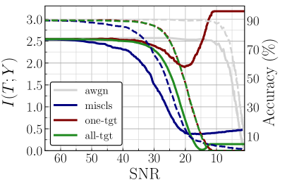
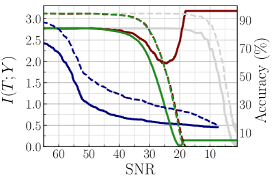
Figure 1: Motivating input-fault tolerance in terms of information conveyed about the original label when models are subject to attacks with different objectives. Model 1 was trained with weight decay, and 1 without. We report $I(T;Y)$ (solid line) and prediction accuracy (dashed line) for a randomly selected subset of 1000 images from the SVHN test set as a function of the SNR in dB for a BIM-$L_{2}$ attack with three different misclassification objectives (details provided in the main text), and AWGN for comparison. Note that for model 1 gradients vanish before zero SNR can be reached.

We begin by demonstrating why it is desirable to examine adversarial attacks from the perspective of the information in the predictions rather than solely evaluating prediction accuracy. Figure 1 shows characteristic curves for two pre-trained models subject to BIM-$L_{2}$ attacks with different adversarial objectives: misclassification “miscls”,which aims to make the prediction not $Y$, and two targeted attack variants, “one-tgt”, which maps each class label to a particular target label (we use the shift $0\rightarrow 1$, $1\rightarrow 2$, …, $9\rightarrow 0$), and “all-tgt”, mapping each original label to each possible incorrect label. For comparison, we also show an additive white Gaussian noise (AWGN) perturbation.

The initial $I(T;Y)$ values for the clean test set are approximately $2.50$ and $2.75$ bits, corresponding to prediction accuracies of $90\%$ and $94\%$ for the model trained with weight decay 1 and without 1, respectively. AWGN is the best-tolerated perturbation, as can be seen from the extended plateau until very low SNR. Furthermore, it is the only one for which $I(T;Y)$ reduces to zero along with the test accuracy. In general, $I(T;Y)$ declines initially as the introduced perturbations cause mistakes in the model’s prediction, but it remains non-zero and behaves distinctly for the three adversarial objectives.

For instance, consider the “one-tgt” case: With increasing perturbation strength the model maps inputs to the target label more consistently. The minimum of this curve marks the transition point at which the perturbed input resembles the target class more closely than its original class. Additional perturbations further refine the input, such that the MI keeps increasing and reaches the upper bound $I(T;Y)=H(Y)$. That is, we observe perfect information transmission despite zero predictive accuracy, indicating that the model’s predictions are in fact correct – the input has been changed to an extent that it is a legitimate member of the target class.

A similar effect occurs for the simpler misclassification case “miscls”, where in Figure 1 we observe a slow increase in $I(T;Y)$ for SNR $\leq 20$, indicating that from this point on additional perturbations systematically add structure to the input. For the case where each wrong label is targeted “all-tgt”, the MI vanishes at the point of complete confusion, i.e., when the inputs are perturbed to the extent that $H(Y|T)=H(Y)$, implying that the probability distribution $p(Y|T)$ is uniform. Additional perturbations beyond this point reduce the probability of the original class to zero, thus causing an “overshoot” effect where $I(T;Y)$ increases to approximately $0.2$ bits, a final saturation value that is independent of the model.

In general, note that targeted attacks require more degradation of the input than a misclassification attack to achieve a desired performance drop; this is reflected in the relative positions of the corresponding curves.

Next, we compare the characteristic MI curves and relate them to model robustness for the case with weight decay, and a baseline without. For the model with weight decay, presented in Figure 1, $I(T;Y)$ is initially slightly lower, but both the decrease and increase in $I(T;Y)$ for the “one-tgt” attack are more gradual than the baseline in Figure 1. Furthermore, the gap between the initial and minimum value is smaller in Figure 1 (approximately $0.50$ vs. $0.75$ bits).

(a)
(b)

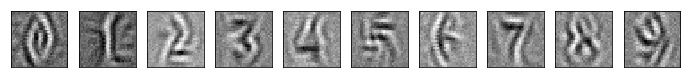
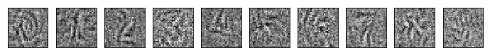
Figure 2: Adversarial examples classified with full confidence 100% that were initialized from white noise. Each of the respective digits are clearly visible in 2 for the more fault tolerant model (trained with weight decay), while only some digits are faintly visible in 2. Results for more SNR values are in Appendix D.

To further connect the gradual degradation property with qualitatively improved robustness to adversarial examples, we use the BIM-$L_{2}$ method to craft “fooling images” [16] for each of the two models, which are shown in Figure 2. Starting from noise drawn from a Gaussian distribution with $\sigma=0.1$, corresponding to an SNR of 20 dB w.r.t. the original ($\sigma=1$) training data, we applied BIM for each target label until full confidence was reached. The resulting images are very different: The model with weight decay, which has a more gradual performance degradation, yields images in Figure 2 that emphasize the edge information relevant to the digit recognition task defined by $Y$. Conversely, the patterns for the baseline in Figure 2 remain contaminated by noise, and do not reflect examples that would be identified by a human with high confidence. Indeed, the model with weight decay classifies the images in Figure 2 with a mean margin of only 28%, while those of Figure 2 are classified with full confidence by the baseline model.

To summarize the analysis presented in Figure 1: Test accuracy consistently degrades to zero with increasing attack strength for all adversarial objectives, while the MI does not. This fact reflects the structure of the learnt clustering of the input space: e.g., class 5 is transformed into an image resembling a “2” more often than it becomes a “1” or a “7”, indicating that the cluster corresponding to “5” is closer to cluster “2” than to the others. The more predictable the alternative incorrect predictions are, the more information $I(T;Y)$ is conveyed. Such insights are lost by the accuracy.

Similar trends are observed under spatial attacks, including rotations and deformations, as shown in Figure 3. Due to the additional digits on the canvas that distract from the center digit for SVHN, we expect rotations and translations to be legitimately confusing for models trained on this dataset. We evaluate the model for $\pm 30^{\circ}$ rotations, as recommended by [8] for $32\times 32$ images, in Figure 3. Translations must be handled with care again due to the peculiarities of the SVHN dataset, where the only difference between otherwise identical images that have a different label can be a translation of just a few pixels.

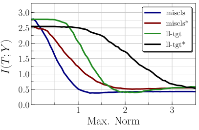
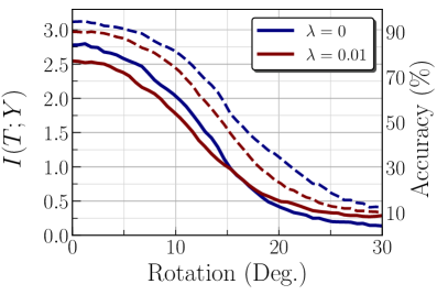
Figure 3: Tolerance to 3 deformations produced by “ADef” for misclassification (“miscls”) and targeting of the least likely label (“ll-tgt”), with accuracy omitted for clarity, and 3 rotations. Models trained with weight decay denoted by “*”. Solid lines show the MI, dashed lines the prediction accuracy. In 3, the maximum permitted norm of the deforming vector field acts as a gauge for the attack strength. In 3, we rotated images by $\leq 30^{\circ}$, as per [8]; beyond this, a significant fraction of the informative pixels were rotated out of the frame and digits were far from their natural orientation.

Finally, we consider attacks capable of producing arbitrary images via deforming vector fields, rather than $L_{p}$ norm-based perturbations of the pixels. The deformation algorithm, “ADef” [1], builds on the first-order DeepFool method [14] to construct smooth deformations through vector fields that are penalized in terms of the supremum norm. The behaviour observed in the tolerance curves of Figure 3 aligns well with results obtained for perturbation-based attacks, where again, training with the weight decay constraint is most compelling, and targeted attacks require greater changes to the input. Several ADef examples and their predictions can be found in Appendix D.

4 Conclusion

We presented a new perspective connecting the adversarial examples problem to fault tolerance — the property that originally motivated the use of neural networks in performance- and safety-critical settings. We introduced a simple and intuitive measure for model tolerance: information transmitted by the model under a given attack strength, which is applicable across a diverse range of realistic fault models. Adversarial examples show that although modern architectures may have some inherent tolerance to internal faults, a combination of subtle design principles and a thorough scope of the intended task are required before they can demonstrate compelling tolerance to input faults.

Acknowledgments

The authors wish to acknowledge the financial support of NSERC, CFI, CIFAR and EPSRC. The authors also acknowledge hardware support from NVIDIA and Compute Canada. Research at the Perimeter Institute is supported by the government of Canada through Industry Canada and by the province of Ontario through the Ministry of Research & Innovation.

Appendix A Additional Detail Regarding the Methodology

It is essential that datasets be prepared identically for model comparison based on the characteristic $I(T;Y)$ vs. SNR curves. As example, presence of a DC offset in the data, which commonly occurs in natural images due to changes in brightness, will shift the SNR curves if not corrected. We suggest adopting the zero-mean, unit-variance standard from image processing, which we implement with per-image mean subtraction in this case for SVHN, after first converting the RGB images to greyscale via NTSC conversion.

Generally speaking, preprocessing that helps with feature learning also helps confer fault tolerance to adversarial attacks. Normally one would also want to linearly decorrelate the pixels in the image, e.g., with ZCA, but we found that the SNR was low enough in many of the SVHN images that this eliminated low frequency gradient information essential for recognizing the digit.

The adversarial examples literature generally leaves the DC component in the dataset by simply normalizing inputs to [0, 1], which is attractive from a simplicity perspective, and convenient for $\epsilon-L_{\infty}$ threat model comparisons, but we find that this practice itself contributes to adverse model behaviour, such as excessively large prediction margins for purely white noise patterns.

Appendix B Additional Fault Tolerance Curves

In Figure 4 we depict the same set of attacks as in Section 3, but for the $L_{\infty}$ variant of BIM. Although Figures 4 and 4 appear qualitatively similar, model 4 trained with weight decay is shifted to the right. By picking SNR values in the range 20–30 and moving upward until intersection with the curves, we see that the degradation is more gradual in Figure 4.

In Figure 5 we show that curves for the $L_{2}$-BIM adversary are generally to the left of those for the $L_{\infty}$-BIM variant. This is expected since the $L_{\infty}$ constraint results in a less efficient adversary for non-linear models.

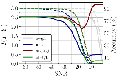
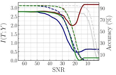
Figure 4: Input-fault tolerance in terms of information $I(T;Y)$ (solid line) and accuracy (dashed line) for 1000 random samples from the SVHN test set, as a function of the SNR for the BIM-$L_{\infty}$ method with three different objectives (see main text for details). As in Figure 1, both models were trained for 50 epochs with 4 weight decay, and 4 without, with the former being more fault tolerant.

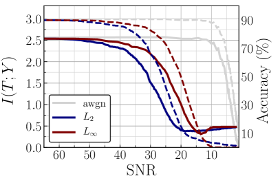
Figure 5: Comparison of BIM-$L_{2}$ and -$L_{\infty}$ misclassification attacks for models trained with 5 weight decay and 5 without. The $L_{\infty}$ variant is less efficient for non-linear models, and thus requires more distortion for a given performance level and is shifted to the right of the $L_{2}$ method.

Appendix C Model Architecture

We use a basic model with four layers, ReLU units, and a Gaussian parameter initialization scheme. Unless specified otherwise, models were trained for 50 epochs with inverse frequency class weighting, constant learning rate (1e-2) SGD with the $L_{2}$ weight decay regularization constant $\lambda$ set to 1e-2 if weight decay is used, and a batch size of 128. We summarize this model in Table 1, and respectively denote $h$, $w$, $c_{in}$, $c_{out}$, $s$ as convolution kernel height, width, number of input and output channels w.r.t. each layer, and stride.

Table 1: Fully-convolutional architecture adapted from the CleverHans library tutorials [17], with 32 filters in first layer instead of 64.

Layer	$h$	$w$	$c_{in}$	$c_{out}$	$s$	params
Conv1	8	8	1	32	2	2.0k
Conv2	6	6	32	64	2	73.8k
Conv3	5	5	64	64	1	102.4k
Fc	1	1	256	10	1	2.6k
Total	–	–	–	–	–	180.9k

Appendix D Adversarial Examples

(a)
(b)
(c)
(d)

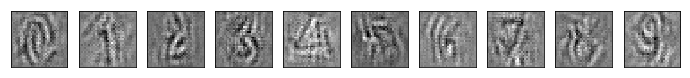
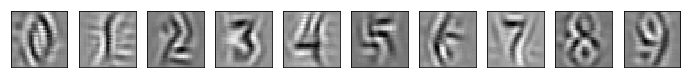
Figure 6: Adversarial “fooling images” classified by a 100% margin that were initialized from white Gaussian noise with $\sigma$=1e-1, or an SNR of 20dB [6–6], and 1e-2, or an SNR of 40dB [6–6] w.r.t. the original training data. Rows 6 and 6 are for the model whose performance degrades more gradually, trained with weight decay.

In Figure 6 we show additional fooling images initialized from noise of varying $\sigma$ or power. For a given value of $\sigma$, the model trained with weight decay yields cleaner images with less task-irrelevant noise.

In Figure 7 we visualize targeted adversarial examples constructed with the BIM-$L_{2}$ approach. In almost all cases, the features of the source digit are manipulated to an extent such that a human observer would likely agree with the target label.

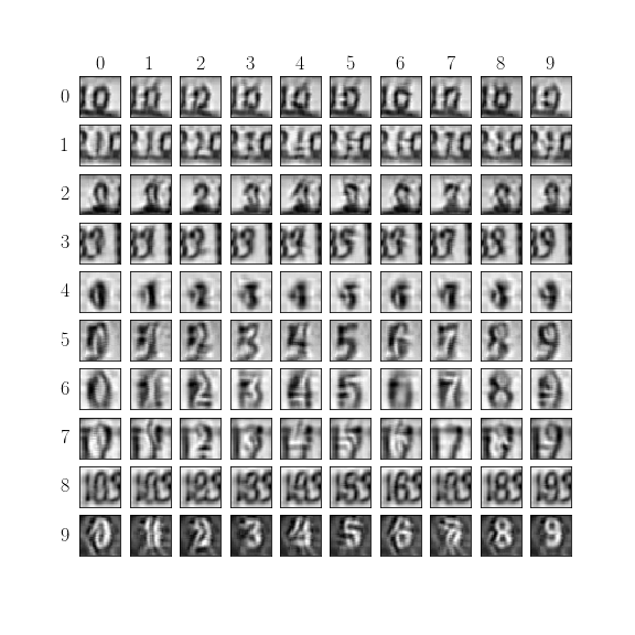
Figure 7: Targeted adversarial examples obtained after running BIM-$L_{2}$ for the least number of iterations sufficient to yield a 91% mean margin. The natural images are enumerated along the diagonal, with the source digit class enumerated vertically, and the target class horizontally.

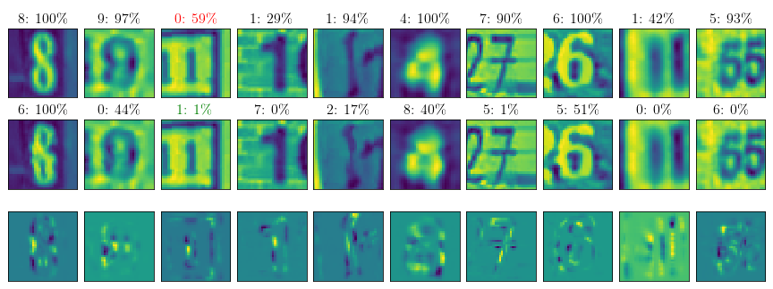
Figure 8: Adversarial deformations constructed with the ADef algorithm, with all incorrect labels as candidates, and max $T$-norm=4, for the model with weight decay. Above each image is the predicted label and prediction margin, defined as the difference between the highest and second-highest softmax values of the prediction. All deformations are concentrated on the edges of the center digit, which is the most relevant information in the image w.r.t. the label. An “8” is deformed into a legitimate “6”, and other instances are in fact ambiguous – e.g., a “1” on a high contrast background could be a “0” with square edges, and “5” is relatively similar to “6” – and are classified by a suitably small margin.

In Figure 8 we supplement the information curves for adversarial deformations, “ADef”, by showing qualitative examples, complete with reasonably interpretable deformations. These examples were not cherry-picked – we arbitrarily sliced a set of ten examples from the test set, and the misclassification confidence was either low, or in the case where examples were misclassified with high confidence, they were usually changed into the target class, e.g., an “8” deformed into a legitimate “6”. It is possible that a different attack, e.g. “stAdv”, may find higher-confidence misclassifications, but these results are nonetheless encouraging and show how attack success rates (100% in Figure 8) can lead to a false sense of vulnerability.

Appendix E The Test Set “Attack”

Our solution achieving roughly 90.4$\pm$0.2% clean test accuracy for the SVHN dataset misses the mark in terms of state-of-the-art results, e.g., 98.70$\pm$0.03% [7]. It was recently suggested that methods which increase the error rate on the test set are more vulnerable to a hypothetical “test set attack”, in which an attacker benefits simply by virtue of typical inputs being misclassified more often [10]. Does such a reduction in test accuracy imply the model is less secure?

Test accuracy is an application-specific constraint, or criteria, which is known during the design phase. Not only can this be communicated in advance to users of the model, it can also be controlled, e.g., by collecting more data, as suggested by [23]. Adversarial examples characterize a situation in which the designer lacks such control for the overwhelming majority of valid inputs, i.e., adversarial subspaces are not usually rare. Such control can be reclaimed by demonstrating fault-tolerance for attacks previously unseen to the model.

Although it is obvious that we should avoid unnecessarily limiting test accuracy, in performance-critical settings we are primarily concerned with behaviour that differs during deployment from that which was observed during the design phase. A model that cannot achieve sufficiently high accuracy should not be deployed in a security sensitive application in the first place, whereas high accuracy on a subset of inputs could lead to a false sense of security, and irrecoverable damages if a product is deployed prematurely.

It is crucial that we communicate precisely what our model does, i.e., is it expected to recognize cars, trucks, and animals in general, or only those appearing in a similar context, and at a given distance from the camera as in a particular database, e.g., the “Tiny Images” [33]. Recent work found test performance degradations of 4–10% absolute accuracy when natural images were drawn from the same database [22], such a large discrepancy in claimed versus obtained performance could be unacceptable in many benign settings, and calls into question the significance of solely numerical improvements on the state-of-the-art. The outlook is likely less promising for the more general recognition case.

The old adage “garbage-in, garbage-out” suggests that we should be at least as rigorous in ensuring models are consistently fed high quality data capable of revealing the intended relationship, as we are rigorous in our threat models. Predicting “birds” versus “bicycles” with no confident mistakes [3] could be difficult to learn from finite data without being more specific about the problem, e.g., is the bird’s whole body in the frame? What is the approximate distance from the camera? Is the bird facing the camera? Our model is expected to recognize any house number depicted with an Arabic numeral from a typical “street-view” distance for the given (unknown) lens, and otherwise yield a low-confidence prediction.

References

- [1] Anonymous. ADef: An Iterative Algorithm to Construct Adversarial Deformations. In Submitted to International Conference on Learning Representations, 2019.
- [2] A. Athalye, N. Carlini, and D. Wagner. Obfuscated Gradients Give a False Sense of Security: Circumventing Defenses to Adversarial Examples. In International Conference on Machine Learning, pages 274–283, 2018.
- [3] T. B. Brown, N. Carlini, C. Zhang, C. Olsson, P. Christiano, and I. Goodfellow. Unrestricted Adversarial Examples. arXiv:1809.08352, 2018.
- [4] N. Carlini and D. Wagner. Towards Evaluating the Robustness of Neural Networks. In IEEE Symposium on Security and Privacy (SP), pages 39–57, 2017.
- [5] P. Chandra and Y. Singh. Fault tolerance of feedforward artificial neural networks- a framework of study. In International Joint Conference on Neural Networks, volume 1, pages 489–494, 2003.
- [6] T. M. Cover and J. A. Thomas. Elements of Information Theory. John Wiley & Sons, Inc., New York, 1991.
- [7] T. DeVries and G. W. Taylor. Improved Regularization of Convolutional Neural Networks with Cutout. arXiv:1708.04552, 2017.
- [8] L. Engstrom, B. Tran, D. Tsipras, L. Schmidt, and A. Madry. A Rotation and a Translation Suffice: Fooling CNNs with Simple Transformations. arXiv:1712.02779, 2017.
- [9] A. Galloway, T. Tanay, and G. W. Taylor. Adversarial Training Versus Weight Decay. arXiv:1804.03308, 2018.
- [10] J. Gilmer, R. P. Adams, I. Goodfellow, D. Andersen, and G. E. Dahl. Motivating the Rules of the Game for Adversarial Example Research. arXiv:1807.06732, 2018.
- [11] I. J. Goodfellow, J. Shlens, and C. Szegedy. Explaining and Harnessing Adversarial Examples. In International Conference on Learning Representations, 2015.
- [12] G. E. Hinton and T. Shallice. Lesioning an attractor network: Investigations of acquired dyslexia. Psychological Review, 98(1):74–95, 1991.
- [13] A. Kurakin, I. J. Goodfellow, and S. Bengio. Adversarial Machine Learning at Scale. International Conference on Learning Representations, 2017.
- [14] S.-M. Moosavi-Dezfooli, A. Fawzi, and P. Frossard. DeepFool: A Simple and Accurate Method to Fool Deep Neural Networks. In The IEEE Conference on Computer Vision and Pattern Recognition (CVPR), 2016.
- [15] Y. Netzer, T. Wang, A. Coates, A. Bissacco, B. Wu, and A. Y. Ng. Reading Digits in Natural Images with Unsupervised Feature Learning. In NIPS Workshop on Deep Learning and Unsupervised Feature Learning, 2011.
- [16] A. Nguyen, J. Yosinski, and J. Clune. Deep neural networks are easily fooled: High confidence predictions for unrecognizable images. In Computer Vision and Pattern Recognition, pages 427–436. IEEE Computer Society, 2015.
- [17] N. Papernot, F. Faghri, N. Carlini, I. Goodfellow, R. Feinman, A. Kurakin, C. Xie, Y. Sharma, T. Brown, A. Roy, A. Matyasko, V. Behzadan, K. Hambardzumyan, Z. Zhang, Y.-L. Juang, Z. Li, R. Sheatsley, A. Garg, J. Uesato, W. Gierke, Y. Dong, D. Berthelot, P. Hendricks, J. Rauber, and R. Long. Technical Report on the CleverHans v2.1.0 Adversarial Examples Library. arXiv:1610.00768, 2018.
- [18] N. Papernot, P. McDaniel, I. Goodfellow, S. Jha, Z. B. Celik, and A. Swami. Practical Black-Box Attacks Against Machine Learning. In Asia Conference on Computer and Communications Security, ASIA CCS, pages 506–519, Abu Dhabi, UAE, 2017. ACM.
- [19] N. Papernot, P. D. McDaniel, S. Jha, M. Fredrikson, Z. B. Celik, and A. Swami. The Limitations of Deep Learning in Adversarial Settings. In IEEE European Symposium on Security and Privacy, pages 372–387, 2016.
- [20] V. Piuri. Analysis of Fault Tolerance in Artificial Neural Networks. Journal of Parallel and Distributed Computing, 61(1):18–48, 2001.
- [21] P. W. Protzel, D. L. Palumbo, and M. K. Arras. Performance and fault-tolerance of neural networks for optimization. IEEE transactions on Neural Networks, 4(4):600–614, 1993.
- [22] B. Recht, R. Roelofs, L. Schmidt, and V. Shankar. Do CIFAR-10 Classifiers Generalize to CIFAR-10? arXiv:1806.00451, 2018.
- [23] L. Schmidt, S. Santurkar, D. Tsipras, K. Talwar, and A. Madry. Adversarially Robust Generalization Requires More Data. arXiv:1804.11285, 2018.
- [24] L. Schott, J. Rauber, M. Bethge, and W. Brendel. Towards the first adversarially robust neural network model on MNIST. arXiv:1805.09190, 2018.
- [25] C. H. Sequin and R. D. Clay. Fault tolerance in artificial neural networks. In International Joint Conference on Neural Networks, volume 1, pages 703–708, 1990.
- [26] C. E. Shannon. A mathematical theory of communication. The Bell System Technical Journal, 27:379–423, 623–656, 1948.
- [27] Y. Sharma and P.-Y. Chen. Attacking the Madry Defense Model with -based Adversarial Examples. arXiv:1710.10733, 2017.
- [28] Y. Song, R. Shu, N. Kushman, and S. Ermon. Constructing Unrestricted Adversarial Examples with Generative Models. In Advances in Neural Information Processing Systems, 2018. To appear.
- [29] N. Srivastava, G. E. Hinton, A. Krizhevsky, I. Sutskever, and R. Salakhutdinov. Dropout: A simple way to prevent neural networks from overfitting. Journal of Machine Learning Research, 15(1):1929–1958, 2014.
- [30] C. Szegedy, W. Zaremba, I. Sutskever, J. Bruna, D. Erhan, I. Goodfellow, and R. Fergus. Intriguing properties of neural networks. In International Conference on Learning Representations, 2014.
- [31] E. B. Tchernev, R. G. Mulvaney, and D. S. Phatak. Investigating the Fault Tolerance of Neural Networks. Neural Computation, 17(7):1646–1664, 2005.
- [32] N. Tishby, F. C. Pereira, and W. Bialek. The information bottleneck method. In Allerton Conference on Communication, Control and Computing, 1999.
- [33] A. Torralba, R. Fergus, and W. T. Freeman. 80 Million Tiny Images: A Large Data Set for Nonparametric Object and Scene Recognition. IEEE Transactions on Pattern Analysis and Machine Intelligence, 30(11):1958–1970, 2008.
- [34] C. Torres-Huitzil and B. Girau. Fault and Error Tolerance in Neural Networks: A Review. IEEE Access, 5:17322–17341, 2017.
- [35] C. Xiao, J.-Y. Zhu, B. Li, W. He, M. Liu, and D. Song. Spatially Transformed Adversarial Examples. In International Conference on Learning Representations, 2018.