Gregory Solid Construction for Polyhedral Volume Parameterization by Sparse Optimization

In isogeometric analysis, it is frequently required to handle the geometric models enclosed by four-sided or non-four-sided boundary patches, such as trimmed surfaces. In this paper, we develop a Gregory solid based method to parameterize those models. First, we extend the Gregory patch representation to the trivariate Gregory solid representation. Second, the trivariate Gregory solid representation is employed to interpolate the boundary patches of a geometric model, thus generating the polyhedral volume parametrization. To improve the regularity of the polyhedral volume parametrization, we formulate the construction of the trivariate Gregory solid as a sparse optimization problem, where the optimization objective function is a linear combination of some terms, including a sparse term aiming to reduce the negative Jacobian area of the Gregory solid. Then, the alternating direction method of multipliers (ADMM) is used to solve the sparse optimization problem. Lots of experimental examples illustrated in this paper demonstrate the effectiveness and efficiency of the developed method.

Key words: Gregory solid, Polyhedral volume parametrization, Sparse optimization, Regularity, Isogeometric analysis

1 Introduction

Isogeometric analysis [1] is an important numerical analysis technique that offers the possibility of integrating computer aided design (CAD) and finite element analysis. While isogeometric analysis requires volumetric representations in some cases, CAD models are usually defined by boundary representations. Therefore, to handle the CAD models defined by boundary representations, they should be transformed into trivariate volumetric representations. However, the transformation of boundary representations into volumetric representations is not trivial, especially when the boundary patches are non-four-sided, (e.g. trimmed surfaces), and the boundary representation model is homeomorphic to a polyhedron, other than hexahedron.

In this paper, we develop a Gregory solid based method to construct the polyhedral volume parametrization of CAD models enclosed by boundary patches, four-sided or non-four-sided. Firstly, the polyhedral parametric domain of the CAD model is constructed, and then split into several hexahedral sub-domains. Secondly, a trivariate Gregory solid mapping from the polyhedral parametric domain to the CAD model is developed to interpolate the boundary patches of the CAD model, thus producing the polyhedral volume parametrization of the CAD model. It is well known that, the volume parametrization that is valid for the isogeometric analysis cannot contain self-intersections or folds, i.e., the mapping should be regular. If the Jacobian [2] of the mapping does not change sign, it is regular. In this paper, the regularity of the Gregory solid mapping is improved by solving a sparse optimization problem which minimizes the negative Jocabian area of the Gregory solid. Finally, the alternating direction method of multipliers [3] (ADMM) method is employed to solve the sparse optimization problem.

This paper is organized as follows: In Section 1.1, we review the related work on Gregory patches, generalized barycentric coordinates, and volumetric parametrization. Section 2 presents the Gregory solid representations. Section 3 develops the optimization problem for improving the parametrization quality. After some experimental results are demonstrated in Section 4, Section 5 concludes this paper.

1.1 Related Work

Triangular mesh parametrization is a commonly employed technique in curve and surface fitting [4], texture mapping [5], remeshing [6], and so on. A triangular mesh parametrization constructs a bijective mapping from the mesh in three dimension to a planar domain. According to the requirements of applications, the frequently used mapping methods in mesh parametrization includes discrete harmonic mapping [4], discrete equiareal mappings [7], and discrete conformal mapping [8]. For more details on triangular mesh parametrization methods and their applications, please refer to [9, 10].

In the field of trivariate solid modeling, the discrete volume parametrization is usually determined by solving a partial differential equation [11, 12] using the finite element method. Lin et al. [13] developed the explicit parametric equations that maps the vertices of a tetrahedral mesh into a parameter domain, thus making the discrete volume parametrization as intuitive and easy to implement as the triangular mesh parametrization methods. In the isogeometric analysis, the three-dimensional physical domains are usually modeled by trivariate B-spline solids, T-spline solids, and subdivision solids, etc., which are generally constructed by filling the CAD models with boundary representation. Wang et al. [14] proposed a method that constructs a T-spline solid from boundary triangulations with arbitrary genus topology by the polycube mapping. In 2013, Xu et al. [15] presented a method to obtain analysis-suitable trivariate NURBS and improve the mesh quality. Zhang et al. [16] developed an approach for volumetric T-spline construction that considers boundary layers. In 2014, an optimization-based approach was developed to generate the B-spline solid with positive Jacobian values from boundary-represented model with six boundary surfaces [17]. In 2015, Lin et al. [13] presented a discrete volume parametrization method for tetrahedral mesh models with six boundary surfaces, and an iterative fitting algorithm for constructing a B-spline solid. In 2018, Lin et al. [18] proposed a method to construct a trivariate B-spline solid by pillow operation and geometric iterative fitting.

To parameterize the mesh vertices of a mesh model with complicated shape for mesh deformation, the generalized barycentric coordinates were developed. In 2002, Meyer et al. [19] presented an easy computation method of a generalized form of barycentric coordinates for irregular, convex n-sided polygons, not only for triangles. Moreover, the mean-value coordinates [20] was developed for both convex and concave polygons, and generalized to 3D polyhedral domains [21]. In 2007, Joshi et al. [22] introduced the harmonic coordinates based on the solutions of the Laplace’s equation, which can work on convex and concave polyhedrons. Because this method does not have a closed form solution, the boundary conditions and the solutions must be defined for every particular case. In 2008, Lipman et al. [23] presented the Green coordinates based on the solution of the Green’s function, which can produce a conformal mapping in 2D and a quasi-conformal mapping in 3D. Note that, nearly all of the generalized barycentric coordinates methods require that the input models are solid. However, the input models handled in this paper are hollowed, enclosed by boundary patches. Therefore, the generalized barycentric coordinates methods cannot be directly used to parameterize the hollowed models handled in this paper.

In this paper, we developed the representation of the trivariate Gregory solid, and employed it to fill the models enclosed by boundary patches, thus generating the polyhedral volume parametrization of the input models. The Gregory patch [24, 25] arose from the Gregory’s method [26], which produces the 8 inner control points from four boundary edges and four corner points, one pair per corner. And then, the four pairs of inner control points are blended so that the generated patch interpolates the boundary straight line segments. Similarly, a triangular Gregory patch can be constructed using the method proposed in [27]. Moreover, Wang et al. [28] defined the Gregory patch as a mapping from an $n$-sided parametric domain with straight line boundaries to an $n$-sided parametric domain of a trimmed surface, and non-self-overlapping structured grids can be generated on it, as well as the trimmed surface.

2 Gregory Solid Representation

Suppose we are given a physical domain, i.e., a curved and hollowed polyhedron $\mathcal{H}$ enclosed by boundary patches. The boundary patches can be any type of parametric surfaces, e.g., parameterized triangular meshes, trimmed surfaces, and so on. In this paper, we develop a Gregory solid representation, and use it to fill the hollowed polyhedron $\mathcal{H}$, thus generating the polyhedral volume parametrization of the polyhedral physical domain. It should be pointed out that, the construction of the Gregory solid requires that each corner of the given polyhedron is adjacent to just three boundary patches. So, in the following, the given polyhedral physical domain $\mathcal{H}$ is supposed to satisfy the requirement.

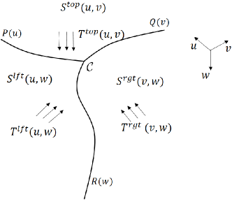
Figure 1: The definition of a Gregory corner interpolator.

2.1 Gregory corner interpolator

The Gregory corner interpolator is defined at each corner of the given polyhedral physical domain $\mathcal{H}$. Suppose $P(u),\ Q(v),\ \text{and}\ R(w),(0\leq u\leq 1,\ 0\leq v\leq 1,\ 0\leq w\leq 1)$ are three boundary curves adjacent to a corner $\mathcal{C}$ of $\mathcal{H}$ (refer to Fig. 1). Whatever the type of the boundary patches adjacent to the corner $\mathcal{C}$ is, we now rewrite them in the form of parametric patches, i.e.,

$$S^{top}(u,v),\ S^{lft}(u,w),\ \text{and}\ S^{rgt}(v,w),\ (0\leq u\leq 1,\ 0\leq v\leq 1,\ 0\leq w\leq 1)$$

which interpolate the three boundary curves (Fig. 1),

$$S^{lft}(u,0)=S^{top}(u,0)=P(u),\ S^{top}(0,v)=S^{rgt}(v,0)=Q(v),\ S^{rgt}(0,w)=S^{lft}(0,w)=R(w).$$

Moreover, we assign the cubic B-spline vector functions $\bar{P}^{lft}(u),\ \bar{P}^{rgt}(u)$ on the boundary curve $P(u)$, the vector functions $\bar{Q}^{lft}(v),\ \bar{Q}^{rgt}(v)$ on the boundary curve $Q(v)$, and the vector functions $\bar{R}^{lft}(w),\ \bar{R}^{rgt}(w)$ on the boundary curve $R(w)$, respectively. The vector functions should satisfy the compatibility conditions,

$$\bar{R}^{rgt}(0)=\bar{Q}^{lft}(0),\ \bar{P}^{rgt}(0)=\bar{R}^{lft}(0),\ \bar{Q}^{rgt}(0)=\bar{P}^{lft}(0).$$

In general, they are generated by approximating the tangent vector functions of the boundary patches at the boundary curves, i.e.,

• $\bar{P}^{lft}(u)$ approximates $\frac{dS^{lft}(u,w)}{dw}\bigg{|}_{w=0}$, and $\bar{P}^{rgt}(u)$ approximates $\frac{dS^{top}(u,v)}{dv}\bigg{|}_{v=0}$;

• $\bar{Q}^{lft}(v)$ approximates $\frac{dS^{top}(u,v)}{du}\bigg{|}_{u=0}$, and $\bar{Q}^{rgt}(v)$ approximates $\frac{dS^{rgt}(v,w)}{dw}\bigg{|}_{w=0}$;

• $\bar{R}^{lft}(w)$ approximates $\frac{dS^{rgt}(v,w)}{dv}\bigg{|}_{v=0}$, and $\bar{R}^{rgt}(w)$ approximates $\frac{dS^{lft}(u,w)}{du}\bigg{|}_{u=0}$.

Then, we construct three bi-cubic B-spline vector functions $T^{top}(u,v),\ T^{lft}(u,w),\ \text{and}\ T^{rgt}(v,w),$ that interpolate the vector functions defined above. Specifically,

• $T^{lft}(u,w)$ interpolates $\bar{R}^{lft}(w)$ and $\bar{P}^{rgt}(u)$;

• $T^{top}(u,v)$ interpolates $\bar{P}^{lft}(u)$ and $\bar{Q}^{rgt}(v)$;

• $T^{rgt}(v,w)$ interpolates $\bar{Q}^{lft}(v)$ and $\bar{R}^{rgt}(w)$.

The bi-cubic B-spline vector functions $T^{top}(u,v),\ T^{lft}(u,w),\ \text{and}\ T^{rgt}(v,w)$ can be written as,

$$\begin{split}T^{top}(u,v)&=\sum\limits_{i=0}^{n_{u}}\sum\limits_{j=0}^{n_{v}}N_{i,p}(u)N_{j,q}(v)X^{top}_{ij},\\ T^{lft}(u,w)&=\sum\limits_{i=0}^{n_{u}}\sum\limits_{k=0}^{n_{w}}N_{i,p}(u)N_{k,r}(w)X^{lft}_{ik},\\ T^{rgt}(v,w)&=\sum\limits_{j=0}^{n_{v}}\sum\limits_{k=0}^{n_{w}}N_{j,q}(v)N_{k,r}(w)X^{rgt}_{jk},\end{split}$$ (1)

where $X^{top}_{ij}$, $X^{lft}_{ik}$ and $X^{rgt}_{jk}$, $i=0,1,...,n_{u},j=0,1,...,n_{v},k=0,1,...,n_{w}$ are control points, and $N_{i,p}(u)$, $N_{j,q}(v)$, $N_{k,r}(w)$ are the basis of B-splines of degree $p$ in the $u$, degree $q$ in the $v$ and degree $r$ in the $w$. In these control points, only the control points of the vector functions

$$\bar{P}^{lft}(u),\ \bar{P}^{rgt}(u),\ \bar{Q}^{lft}(v),\ \bar{Q}^{rgt}(v),\ \bar{R}^{lft}(w),\ \text{and}\ \bar{R}^{rgt}(w)$$

are known, and the other control points are unknown. They will be taken as variables in the optimization procedure stated in Section 3, and determined by solving the optimization problem.

Remark 1 (Construction of the initial patches).

In solving the optimization problem developed in Section 3, the initial patches of $T^{top}(u,v),\ T^{lft}(u,w)$, and $T^{rgt}(v,w)$ are required. Take the construction of the initial representation of $T^{top}(u,v)$ as an example. As stated above, $T^{top}(u,v)$ should interpolate the two curves $\bar{P}^{lft}(u)$ and $\bar{Q}^{rgt}(v)$, which are two boundary curves of $T^{top}(u,v)$. In order to produce the other two boundary curves of $T^{top}(u,v)$, we first construct a corner,

$$\mathcal{C}_{p}=\frac{\bar{P}^{lft}(1)+\bar{Q}^{rgt}(1)}{2}+2\left(\frac{\bar{P}^{lft}(1)+\bar{Q}^{rgt}(1)}{2}-\bar{P}^{lft}(0)\right),$$

and then, connect the two corners $\bar{P}^{lft}(1)$ and $\mathcal{C}_{p}$, and the two corners $\bar{Q}^{rgt}(1)$ and $\mathcal{C}_{p}$, thus generating two line segments as the other two boundary curves of $T^{top}(u,v)$. In this way, we get four boundary curves, and a bilinear patch can be generated by bilinear interpolation to the four boundary curves. Moreover, by degree elevation, the bilinear patch becomes a bi-cubic B-spline patch, which can be taken as the initial patch of $T^{top}(u,v)$. The initial patches of $T^{lft}(u,w)$ and $T^{rgt}(v,w)$ can be constructed in the similar manner.

In conclusion, the Gregory corner interpolator with respect to the corner $\mathcal{C}$ that interpolates

$$\{S^{top}(u,v),S^{lft}(u,w),S^{rgt}(v,w),T^{top}(u,v),T^{lft}(u,w),T^{rgt}(v,w)\}$$

can be represented as,

$$\begin{split}R&(u,v,w)=[1\quad w]{\left[\begin{array}[]{c}S^{top}(u,v)\\ T^{top}(u,v)\\ \end{array}\right]}+[1\quad v]{\left[\begin{array}[]{c}S^{lft}(u,w)\\ T^{lft}(u,w)\\ \end{array}\right]}+[1\quad u]{\left[\begin{array}[]{c}S^{rgt}(v,w)\\ T^{rgt}(v,w)\\ \end{array}\right]}\\ &-[1\quad u]{\left[\begin{array}[]{cc}S^{lft}(0,w)&T^{lft}(0,w)\\ T^{rgt}(0,w)&\frac{vT^{lft}_{u}(0,w)+uT^{rgt}_{v}(0,w)}{u+v}\\ \end{array}\right]}{\left[\begin{array}[]{c}1\\ v\\ \end{array}\right]}\\ &-[1\quad v]{\left[\begin{array}[]{cc}S^{top}(u,0)&T^{top}(u,0)\\ T^{lft}(u,0)&\frac{vT^{lft}_{w}(u,0)+wT^{top}_{v}(u,0)}{v+w}\\ \end{array}\right]}{\left[\begin{array}[]{c}1\\ w\\ \end{array}\right]}\\ &-[1\quad w]{\left[\begin{array}[]{cc}S^{rgt}(v,0)&T^{rgt}(v,0)\\ T^{top}(0,v)&\frac{uT^{rgt}_{w}(v,0)+wT^{top}_{u}(0,v)}{u+w}\\ \end{array}\right]}{\left[\begin{array}[]{c}1\\ u\\ \end{array}\right]}\\ &+\mathcal{T}_{ijk}u^{i}v^{j}w^{k},\end{split}$$ (2)

where the Einstein’s summation convention is applied in the last term,

$$u^{0}=1,\ u^{1}=u,\ v^{0}=1,\ v^{1}=v,\ w^{0}=1,\ w^{1}=w,$$

and $\mathcal{T}_{ijk}$ is a 3-order tensor with elements, $\mathcal{T}_{000}=S^{top}(0,0)$,  $\mathcal{T}_{100}=T^{rgt}(0,0)$,  $\mathcal{T}_{010}=T^{lft}(0,0)$,  $\mathcal{T}_{001}=T^{top}(0,0)$,
$\mathcal{T}_{110}=\frac{vT^{lft}_{u}(0,0)+uT^{rgt}_{v}(0,0)}{u+v}$,  $\mathcal{T}_{011}=\frac{vT^{lft}_{w}(0,0)+wT^{top}_{v}(0,0)}{v+w}$,  $\mathcal{T}_{101}=\frac{uT^{rgt}_{w}(0,0)+wT^{top}_{u}(0,0)}{u+w}$,
$\mathcal{T}_{111}=\frac{uv(uT^{rgt}_{vw}(0,0)+vT^{lft}_{uw}(0,0))+uw(uT^{rgt}_{wv}(0,0)+wT^{top}_{uv}(0,0))+vw(vT^{lft}_{wu}(0,0)+wT^{top}_{vu}(0,0))}{uv(u+v)+uw(u+w)+vw(v+w)}$.
Here, $T^{rgt}_{v}(v,w)$ denotes the first order partial derivative $\frac{\partial T^{rgt}(v,w)}{\partial v}$, $T^{rgt}_{wv}(v,w)$ denotes the second order partial derivative $\frac{\partial^{2}T^{rgt}(v,w)}{\partial w\partial v}$, and so on. It is easy to be validated that, the Gregory corner interpolator (2) interpolates the three boundary patches adjacent to the corner $\mathcal{C}$, i.e.,

$$R(u,v,0)=S^{top}(u,v),R(u,0,w)=S^{lft}(u,w),\text{and}\ R(0,v,w)=S^{rgt}(v,w),$$

and its partial derivatives satisfy,

$$\frac{\partial R(u,v,w)}{\partial w}\bigg{|}_{w=0}=T^{top}(u,v),\quad\frac{\partial R(u,v,w)}{\partial v}\bigg{|}_{v=0}=T^{lft}(u,w),\quad\frac{\partial R(u,v,w)}{\partial u}\bigg{|}_{u=0}=T^{rgt}(v,w).$$

As stated above, the Gregory corner interpolator (2) is defined at each corner of the given polyhedral physical domain $\mathcal{H}$. The Gregory solid representation is the weighted sum of the Gregory corner interpolators at all of the corners of $\mathcal{H}$, which will be presented in Section 2.3.

2.2 Parametric domain

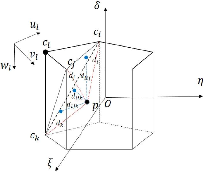
Figure 2: The calculation of the parameter values $(u_{l},v_{l},w_{l})$ of the point $p$ with respect to the corner $c_{l}$ of the pentagonal prism parametric domain $\mathcal{P_{G}}$.

Before constructing the Gregory solid $\mathcal{G}$ that interpolates the boundary patches of the polyhedral physical domain $\mathcal{H}$, its parametric domain $\mathcal{P_{G}}$ should be firstly specified. The parametric domain $\mathcal{P_{G}}$ is a polyhedron in the $\xi-\eta-\delta$ parametric space (refer to Fig. 2), which is determined by the number of the boundary patches of the physical domain $\mathcal{H}$. For example, if $\mathcal{H}$ has four boundary patches, the parametric domain $\mathcal{P_{G}}$ of the Gregory solid is a tetrahedron. In Fig. 2, a pentagonal prism parametric domain is illustrated, and the corresponding physical domain $\mathcal{H}$ has seven boundary patches. In our implementation, the edges of the parametric domain $\mathcal{P_{G}}$ (a polyhedron) are unit length.

Given a point $p=(\xi,\eta,\delta)\in\mathcal{P_{G}}$, it has parameter values in each Gregory corner interpolator (2). So, the parameter values for the point $p=(\xi,\eta,\delta)$ should be defined with respect to each corner of $\mathcal{P_{G}}$. Refer to Fig. 2, the parameter values $(u_{l},v_{l},w_{l})$ of the point $p=(\xi,\eta,\delta)$ with respect to the corner $c_{l}$ is constructed according to the following manner. Consider the tetrahedron $c_{l}-c_{i}c_{j}c_{k}$. On one hand, denote the distances from the point $p=(\xi,\eta,\delta)$ to the planes determined by the triangular faces $\triangle c_{l}c_{i}c_{k}$, $\triangle c_{l}c_{i}c_{j}$, and $\triangle c_{l}c_{j}c_{k}$ are $d_{lik},\ d_{lij},\ d_{ljk}$, respectively. On the other hand, denote the distances from the point $p=(\xi,\eta,\delta)$ to the three corners $c_{i},\ c_{j}$, and $c_{k}$ are $d_{i},\ d_{j}$, and $d_{k}$, respectively. The parameter values $(u_{l},v_{l},w_{l})$ of the point $p=(\xi,\eta,\delta)$ with respect to the corner $c_{l}$ is defined as,

$$(u_{l},v_{l},w_{l})=\left(\frac{d_{ljk}}{d_{ljk}+d_{i}},\frac{d_{lik}}{d_{lik}+d_{j}},\frac{d_{lij}}{d_{lij}+d_{k}}\right).$$

It can be easily checked that,

• if the point $p$ is at the corner $c_{l}$, we have $(u_{l},v_{l},w_{l})=(0,0,0)$;

• if the point $p$ is at the corner $c_{i}$, we have $(u_{l},v_{l},w_{l})=(0,0,1)$;

• if the point $p$ is at the corner $c_{j}$, we have $(u_{l},v_{l},w_{l})=(1,0,0)$;

• if the point $p$ is at the corner $c_{k}$, we have $(u_{l},v_{l},w_{l})=(0,1,0)$;

• if the point $p$ is in the line $c_{l}c_{i}$, we have $u_{l}=v_{l}=0$;

• if the point $p$ is in the line $c_{l}c_{j}$, we have $v_{l}=w_{l}=0$;

• if the point $p$ is in the line $c_{l}c_{k}$, we have $u_{l}=w_{l}=0$;

• if the point $p$ is on the plane determined by $\triangle c_{l}c_{i}c_{k}$, we have $u_{l}=0$;

• if the point $p$ is on the plane determined by $\triangle c_{l}c_{i}c_{j}$, we have $v_{l}=0$;

• if the point $p$ is on the plane determined by $\triangle c_{l}c_{j}c_{k}$, we have $w_{l}=0$.

2.3 Gregory solid representation

Given a polyhedral physical domain $\mathcal{H}$ with $n$ corners. In this section, we will develop the representation of the Gregory solid $\mathcal{G}$ that fills the physical domain $\mathcal{H}$, and interpolates its boundary patches at the same time. Accordingly, the parametric domain $\mathcal{P_{G}}$ of $\mathcal{G}$ also has $n$ corners $c_{l},l=0,1,\cdots,n-1$. Moreover, suppose it has $m$ faces $f_{i},i=0,1,\cdots,m$. For a point $p=(\xi,\eta,\delta)\in\mathcal{P_{G}}$, denoting $d(p,f_{i})$ as the distance from the point $p$ to the face $f_{i},i=0,1,\cdots,m$, the weight function $W_{l}(p)$ for the corner $c_{l},l=0,1,\cdots,n-1$ can be defined as,

$$W_{l}(p)=\frac{\prod_{\text{$f_{i}$ is not adjacent to $c_{l}$}}d^{2}(p,f_{i})}{\sum_{j=0}^{n-1}\prod_{\text{$f_{i}$ is not adjacent to $c_{j}$}}d^{2}(p,f_{i})},\ p\in\mathcal{P_{G}}.$$ (3)

Then, the Gregory solid $\mathcal{G}(p):\mathcal{P_{G}}\rightarrow\mathcal{H}$ can be defined as the weighted sum of the $n$ corner interpolator functions,

$$\mathcal{G}(p)=\sum_{l=0}^{n-1}W_{l}(p)R_{l}(u_{l}(p),v_{l}(p),w_{l}(p)),$$ (4)

where $R_{l}(u_{l}(p),v_{l}(p),w_{l}(p))$ is the Gregory corner interpolator (2) to the $l^{th}$ corner $c_{l},l=0,1,\cdots,n-1$.

It should be pointed out that, $W_{l}(p)=1$ if $p$ is at the corner $c_{l}$, and $W_{l}(p)$ is zero if $p$ is on the faces not adjacent to the corner $c_{l}$. Therefore, the Gregory solid $\mathcal{G}(p)$ interpolates the boundary patches of the physical domain $\mathcal{H}$. Specifically, if $p_{1}$ is on a face of the parametric domain $\mathcal{P_{G}}$, then there is a point $q_{1}$ on a corresponding boundary patch of $\mathcal{H}$ such that $\mathcal{G}(p_{1})=q_{1}$. On the contrary, if there is a point $q_{2}$ on a boundary patch of $\mathcal{H}$, then there exists a point $p_{2}$ on a corresponding face of $\mathcal{P_{G}}$ such that $\mathcal{G}(p_{2})=q_{2}$.

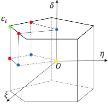
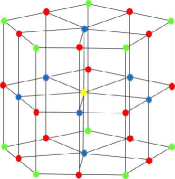
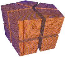
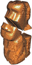
Figure 3: Parametric grid generation. (a) Dual operation for a corner. (b) Parametric domain after dual operation. (c) Parametric domain discretization (separated). (d) Parametric grid in the physical domain (separated).

2.4 Parametric grid generation

Now, we have constructed a Gregory solid $\mathcal{G}(p),\ p\in\mathcal{P_{G}}$ which fills the polyhedral physical domain $\mathcal{H}$, and interpolates its boundary patches. The Gregory solid $\mathcal{G}(p)$ can be considered as a mapping from its parametric domain $\mathcal{P_{G}}$ to the physical domain $\mathcal{H}$, i.e., $\mathcal{G}(p):\mathcal{P_{G}}\rightarrow\mathcal{H}$. Then, the parametric grid in the physical domain $\mathcal{H}$ can be generated by the Gregory solid mapping.

Suppose the parametric domain $\mathcal{P_{G}}$ has $n$ corners. In order to produce the parametric grid, the parametric domain $\mathcal{P_{G}}$ is first segmented into $n$ hexahedra using the dual operation (Algorithm 1), each hexahedron for a corner (Fig. 3). Then, each hexahedron is uniformly discretized into a $M\times N\times L$ grid (Fig. 3). For conformity, on the common face of two adjacent hexahedra, the discretization is taken the same manner, resulting in the same grid. Finally, the grids in the parametric domain $\mathcal{P_{G}}$ is mapped into the physical domain $\mathcal{H}$ by the Gregory mapping $\mathcal{G}(p):\mathcal{P_{G}}\rightarrow\mathcal{H}$, thus generating the parametric grid in the physical domain (Fig. 3).

Algorithm 1 Dual operation (refer to Fig. 3)

1:  Calculate the middle point of every edge of the polyhedral parametric domain $\mathcal{P_{G}}$;

2:  Calculate the barycenter of every face of $\mathcal{P_{G}}$;

3:  Calculate the barycenter of $\mathcal{P_{G}}$;

4:  Construct a hexahedron for each corner $c_{l}$ of $\mathcal{P_{G}}$, by linking the eight points, i.e., the middle points of the three edges adjacent to $c_{l}$, the barycenters of the three faces adjacent to $c_{l}$, the barycenter of $\mathcal{P_{G}}$, and the corner $c_{l}$ (refer to Fig. 3, and 3).

3 Optimization

In this section, we develop a sparse optimization model to improve the algebraic quality, i.e., the quality of the parametrization, of the Gregory solid constructed in Section 2. In order to employ the sparse optimization technique, the formulation of the objective function is based on the parametric grid generated using the method developed in Section 2.4.

It is well known that, a trivariate solid is valid in isogeometric analysis if its Jacobian is positive at any point. Note that the parametric grid in the physical domain $\mathcal{H}$ is a hexahedral mesh (Fig. 3), and the Jacobian of a hexahedral mesh is defined for each vertex of each hexahedron. Specifically, give the $s^{th}(s=0,1,\cdots,K)$ hexahedron of the hexahedral mesh with vertices $P_{h}=(x_{h},y_{h},z_{h}),\ h=0,1,\cdots,7$, and suppose $P_{i}=(x_{i},y_{i},z_{i}),\ P_{j}=(x_{j},y_{j},z_{j}),\ P_{k}(x_{k},y_{k},z_{k}),$ are the three vertices adjacent to the vertex $P_{h}=(x_{h},y_{h},z_{h})$. The order of the vertices of the tetrahedron $P_{h}-P_{i}P_{j}P_{k}$ is arranged in some specified orientation (clockwise or counterclockwise), so that the majority of Jacobians are positive. The scaled Jacobian at the vertex $P_{h},\ h=0,1,\cdots,7$ of the $s^{th}$ hexahedron is defined as [2],

$$J^{s}_{h}=det\left(\begin{array}[]{cccc}\frac{x_{i}-x_{h}}{\left\|\overrightarrow{P_{i}P_{h}}\right\|_{2}}&\frac{x_{j}-x_{h}}{\left\|\overrightarrow{P_{j}P_{h}}\right\|_{2}}&\frac{x_{k}-x_{h}}{\left\|\overrightarrow{P_{k}P_{h}}\right\|_{2}}\\ \frac{y_{i}-y_{h}}{\left\|\overrightarrow{P_{i}P_{h}}\right\|_{2}}&\frac{y_{j}-y_{h}}{\left\|\overrightarrow{P_{j}P_{h}}\right\|_{2}}&\frac{y_{k}-y_{h}}{\left\|\overrightarrow{P_{k}P_{h}}\right\|_{2}}\\ \frac{z_{i}-z_{h}}{\left\|\overrightarrow{P_{i}P_{h}}\right\|_{2}}&\frac{z_{j}-z_{h}}{\left\|\overrightarrow{P_{j}P_{h}}\right\|_{2}}&\frac{z_{k}-z_{h}}{\left\|\overrightarrow{P_{k}P_{h}}\right\|_{2}}\end{array}\right),\ h=0,1,\cdots,7,\ s=0,1,\cdots,K,$$

where $\left\|\cdot\right\|_{2}$ is the 2-norm of a vector. Thus, the scaled Jacobians for the parametric grid of the physical domain $\mathcal{H}$ can be organized in a vector $Jac$,

$$Jac=[J^{0}_{0},J^{0}_{1},\cdots,J^{0}_{7},\cdots,J^{K}_{0},J^{K}_{1},\cdots,J^{K}_{7}].$$ (5)

Moreover, by defining two functions,

$$\begin{array}[]{ccc}pos(J^{s}_{h})=\begin{cases}J^{s}_{h},&J^{s}_{h}\geq 0,\\ 0&J^{s}_{h}<0,\end{cases}&\qquad\text{and}&neg(J^{s}_{h})=\begin{cases}0,&J^{s}_{h}>0,\\ J^{s}_{h}&J^{s}_{h}\leq 0,\end{cases}\end{array}$$

the Jacobian vector $Jac$ (5) can be decomposed into two parts, i.e.,

$$Jac=Jac^{+}+Jac^{-},$$

where,

$$Jac^{+}=[pos(J^{0}_{0}),pos(J^{0}_{1}),\cdots,pos(J^{0}_{7}),\cdots,pos(J^{K}_{0}),pos(J^{K}_{1}),\cdots,pos(J^{K}_{7})]$$ (6)

contains the positive and zero elements of the vector $Jac$ (5), and

$$Jac^{-}=[neg(J^{0}_{0}),neg(J^{0}_{1}),\cdots,neg(J^{0}_{7}),\cdots,neg(J^{K}_{0}),neg(J^{K}_{1}),\cdots,neg(J^{K}_{7})]$$ (7)

contains the negative and zero elements of the vector $Jac$ (5).

On one hand, to improve the validity of the Gregory solid, two objective functions are required. First, the less the number of the vertices with negative Jacobian, the better the validity, which is formulated as the sparse optimization objective function,

$$E_{sparse}=\left\|Jac^{-}\right\|_{0},$$ (8)

where $\left\|Jac^{-}\right\|_{0}$ is the 0-norm of $Jac^{-}$, that is, the number of nonzero elements of the vector $Jac^{-}$. Second, the larger the sum of the positive Jacobians, the better the validity, which is modelled as the following objective function (refer to (5)),

$$E_{positive}=\sum_{J^{s}_{h}\geq 0}\frac{1}{J^{s}_{h}+\epsilon}.$$ (9)

Experiments show that $\epsilon=10^{-5}$ can lead to desirable results.

On the other hand, to improve the smoothness of the parametric grid of the physical domain $\mathcal{H}$, the Laplace smoothing function is taken as an objective function,

$$E_{smooth}=\sum_{i}\left\|P_{i}-\frac{1}{\#N(P_{i})}\sum_{P_{j}\in N(P_{i})}P_{j}\right\|_{2}^{2},$$ (10)

where $P_{i}$ is a vertex of the parametric grid, $N(P_{i})$ denotes the set of one-ring adjacent vertices to $P_{i}$, and $\#N(P_{i})$ is the number of the one-ring adjacent vertices to $P_{i}$.

Consequently, the whole objective function $E$ is taken as a linear combination of the three aforementioned objective functions,

$$E=E_{smooth}+\mu E_{positive}+\nu E_{sparse},$$

where the weights $\mu>0$ and $\nu>0$ are utilized to balance the three items. Returning to the Gregory solid representation (4), we can see that the variables that can be adjusted for improving the parametric quality are the control points of the three bi-cubic B-spline vector functions $T^{top}(u,v)$, $T^{lft}(u,w)$, and $T^{rgt}(v,w)$ (1). Denoting the set of these control points as $X$, the whole optimization problem can be formulated as,

$$\begin{split}\min_{X}\sum_{i}\left\|P_{i}-\frac{1}{\#N(P_{i})}\sum_{P_{j}\in N(P_{i})}P_{j}\right\|_{2}^{2}+\mu\sum_{J^{s}_{h}\geq 0}\frac{1}{J^{s}_{h}+\epsilon}+\nu\left\|Jac^{-}\right\|_{0}.\end{split}$$ (11)

In fact, for the convenience of the optimization problem (11) to be solved by the alternating direction method of multipliers (ADMM) [3], the $0-$norm of the sparse item is replaced by the $1-$norm, and the optimization problem is changed to,

$$\begin{split}&\min_{X,Y,Z}\sum_{i}\left\|P_{i}(X)-\frac{1}{\#N(P_{i})}\sum_{P_{j}\in N(P_{i})}P_{j}(X)\right\|_{2}^{2}+\mu\sum_{J^{s}_{h}\geq 0}\frac{1}{J^{s}_{h}(Y)+\epsilon}+\nu\left\|Jac^{-}(Z)\right\|_{1}\\ &s.t.\quad X=Y=Z.\end{split}$$ (12)

Then, we can develop the format of ADMM for solving the above optimization problem (12),

$$X^{t+1} \leftarrow\arg\min_{X}\left(\sum_{i}\left\|P_{i}(X)-\frac{1}{\#N(P_{i})}\sum\limits_{P_{j}\in N(P_{i})}P_{j}(X)\right\|_{2}^{2}+\frac{\rho}{2}\left\|\begin{bmatrix}X\\ X\end{bmatrix}-\begin{bmatrix}Y^{t}\\ Z^{t}\end{bmatrix}+\begin{bmatrix}U_{Y}^{t}\\ U_{Z}^{t}\end{bmatrix}\right\|^{2}_{2}\right),$$ (13)

$$Y^{t+1} \leftarrow\arg\min_{Y}\left(\mu\sum_{J^{s}_{h}\geq 0}\frac{1}{J^{s}_{h}(Y)+\epsilon}+\frac{\rho}{2}\|X^{t+1}-Y+U_{Y}^{t}\|^{2}_{2}\right),$$ (14)

$$\ Z^{t+1} \leftarrow\arg\min_{Z}\left(\nu\left\|Jac^{-}(Z)\right\|_{1}+\frac{\rho}{2}\left\|X^{t+1}-Z+U_{Z}^{t}\right\|^{2}_{2}\right),$$ (15)

$$U^{t+1} \leftarrow U^{t}+\rho\left(\begin{bmatrix}X^{t+1}\\ X^{t+1}\end{bmatrix}-\begin{bmatrix}Y^{t+1}\\ Z^{t+1}\end{bmatrix}\right),$$ (16)

$$t=0,1,2,\cdots$$ (17)

where the factor $\rho$ is a penalty parameter, and $\rho=1$ is a desirable selection for fast convergence. The initial values $X^{0}=Y^{0}=Z^{0}$ are constructed by the method presented in Remark 1, and we set $U^{0}=0$. In the ADMM format developed above, each individual updating step is a small optimization itself, and can be solved efficiently. Specifically, in our implementation, the gradient descent method [29] is employed to solve the first optimization problem (13), and the sub-gradient descent method [29] is adopted to solve the second (14) and the third optimization problem (15).

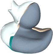
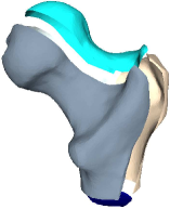
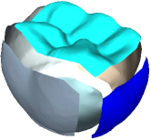
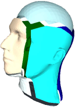
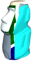
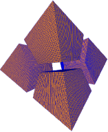
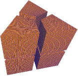
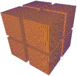
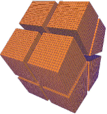
Figure 4: The input mesh models, Duck(a), Ball joint(b), Tooth(c), Head(d), and Moai(e); their separated parametrization domain: tetrahedron (f), pentahedron (triangular prism) (g), hexahedron (h), heptahedron (pentagonal prism)(i), and heptahedron (pentagonal prism)(j).

4 Results and discussions

In this section, some experimental results are illustrated to demonstrate the effectiveness and efficiency of the Gregory solid construction and optimization algorithm developed above. All of the experimental examples are run on a PC with 3.60GHz CPU i7-4790 and 16G memory. As stated in Section 2, the input to our algorithm is a polyhedral hollowed physical domain $\mathcal{H}$, where each corner is adjacent to just three boundary patches. Although the boundary patches can be any type of parametric surfaces, in our experiments, triangular meshes are taken as the boundary patches. Moreover, we employ the conformal parametrization method [4] to calculate their parametrization. Thus, the triangular meshes become parametric surfaces with their parametrization.

In Fig. 4, the input polyhedral physical domains and the parametric domains of the corresponding Gregory solids are illustrated. While the input physical domains are demonstrated in Figs. 4(a)-(e), the parametric domains of the corresponding Gregory solids are presented in Figs. 4(f)-(j). Specifically, the models illustrated in Fig.4(a)-(e) are Duck, Ball Joint, Tooth, Head, and Moai, respectively, and their parametric domains are tetrahedron (Fig. 4(f)), pentahedron (triangular prism, Fig. 4(g)), hexahedron (Fig. 4(h)), heptahedron (pentagonal prism, Fig. 4(i)), and heptahedron (pentagonal prism, Fig. 4(j)), respectively. Additionally, for each input model, the numbers of mesh vertices, triangular faces, and boundary patches are listed in Table 1. It can be seen that, the numbers of mesh vertices range from 3928 to 15154, and the numbers of faces from 7852 to 30304.

Table 1: Statistical data of the Gregory solids generation method developed in this paper.

model	#vert.1	#face2	#boundary3	#grid4	avg.J.5	min.J.5	max.J.5	$J^{-}/J$ 6	time7
Duck	10461	20918	4	$30\times 30\times 30$	0.8006	-0.5763	0.9995	0.176%	2386.22
Ball joint	10936	21868	5	$26\times 26\times 26$	0.8009	-0.1495	0.9991	0.071%	1820.22
Tooth	15154	30304	6	$15\times 15\times 15$	0.9362	0.0133	0.9999	0	130.22
Head	3928	7852	7	$16\times 16\times 16$	0.8428	-0.4752	0.9997	0.172%	1219.87
Moai	5685	11366	7	$18\times 18\times 18$	0.8881	-0.4693	0.9999	0.014%	1180.88

• Number of vertices of the input triangular mesh model.

• Number of faces of the input triangular mesh model.

• Number of boundary patches of the physical domain.

• Resolution of the discretized grid in each segmented parametric sub-domain.

• Average, minimal, and maximal scaled Jacobian values.

• Ratio between the volume of region with negative Jacobian and the volume of the whole model.

• Running time in seconds.

In Fig. 5(a)-(e), the polyhedral volume parametric mesh generated by the Gregory solid mapping are illustrated, with their cut-away views (Fig. 5(f)-(j)). The average, minimal, and maximal scaled Jacobians of these Gregory solids are listed in Table 1. The average scaled Jacobians of the Gregory solids are all above $0.8$. Although there are still some regions with negative Jacobians in four models, the ratio between the volume of region with negative Jacobian and the volume of the whole model are below $0.18\%$ (refer to the column of $J^{-}/J$ in Table 1). Further checking shows that the regions with negative Jacobian concentrate on the regions near the inappropriately segmented boundary patches, for example, two adjacent boundary patches are $C^{1}$ continuous along their common boundary curve.

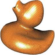
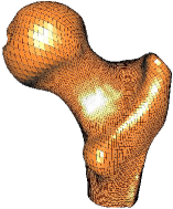
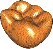
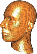
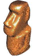
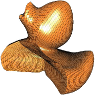
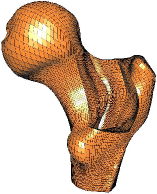
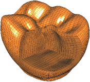
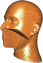
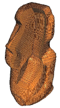
Figure 5: The polyhedral volume parametric mesh in the physical domains Duck (a), Ball joint (b), Tooth (c), Head (d), and Moai (e), and their cut away views (f), (g), (h), (i), (j).

Moreover, the last column of Table 1 lists the running time of the Gregory solid construction and optimization algorithm, ranging from 130.22 seconds to 2386.22 seconds. Specially, we can see that the tooth model has no region with negative Jacobian after optimization and the running time of optimization is much shorter than others, because of the segmentation of tooth model and the initial generated hexahedral model is much better than others. There is still some space for accelerating the algorithm. In Table 2, the weights $\mu$ and $\nu$ (in the objective function (11)) employed in generating each Gregory solid are presented. As stated above, the weights $\mu$ and $\nu$ are used to balance the values of the three items in the objective function (11). Because the orders of magnitude of the three items differ in the optimization of each Gregory solid, the weights $\mu$ and $\nu$ also differ in each optimization.

Table 2: Weights employed in optimization.

	Duck	Ball joint	Tooth	Head	Moai
$\mu$	0.000001	0.00001	0.00001	0.000001	0.00002
$\nu$	0.3	0.1	0.01	0.03	0.02

5 Conclusion

In this paper, we developed the Gregory solid representation, and employed it to interpolate the four-sided or non-four-sided boundary patches of a polyhedral physical domain. Moreover, the algebraic quality of the Gregory solid is improved by solving a sparse optimization problem using the ADMM method. In this way, the polyhedral volume parametrization of a given physical domain with four-sided or non-four-sided boundary patches can be generated. Experiments show that, in the polyhedral volume parametrization produced by the Gregory solid construction and sparse optimization method, the regions with negative Jacobian are very small (below 0.18%), and they usually concentrate around the boundary curves where two boundary patches are $C^{1}$ continuously stitched. As a future work, we will study how to entirely eliminate the region with negative Jacobian by optimizing the boundary patch segmentation.

References

- [1] T. J. R. Hughes, J. A. Cottrell, and Y. Bazilevs. Isogeometric analysis: Cad, finite elements, nurbs, exact geometry and mesh refinement. Computer Methods in Applied Mechanics & Engineering, 194(39):4135–4195, 2005.
- [2] Patrick M Knupp. Achieving finite element mesh quality via optimization of the jacobian matrix norm and associated quantities. part ii a framework for volume mesh optimization and the condition number of the jacobian matrix. International Journal for Numerical Methods in Engineering, 48(8):1165–1185, 2000.
- [3] Stephen Boyd, Neal Parikh, Eric Chu, Borja Peleato, and Jonathan Eckstein. Distributed optimization and statistical learning via the alternating direction method of multipliers. Foundations & Trends in Machine Learning, 3(1):1–122, 2010.
- [4] Michael S Floater. Parametrization and smooth approximation of surface triangulations. Computer Aided Geometric Design, 14(3):231–250, 1997.
- [5] Pedro V. Sander, John Snyder, Steven J. Gortler, and Hugues Hoppe. Texture mapping progressive meshes. pages 409–416, 2001.
- [6] Pierre Alliez, Giuliana Ucelli, Craig Gotsman, and Marco Attene. Recent advances in remeshing of surfaces. Mathematics & Visualization, pages 53–82, 1970.
- [7] K Hormann. Mips : An efficient global parametrization method. Curve and Surface Design: Saint-Malo, 2000.
- [8] Jos Mar a Las Heras. An adaptable surface parameterization method. Proceedings of International Meshing Roundtable, (7):201–213, 2003.
- [9] Michael S. Floater and Hormann Kai. Surface Parameterization: a Tutorial and Survey. Springer Berlin Heidelberg, 2005.
- [10] Alla Sheffer, Emil Praun, and Kenneth Rose. Mesh parameterization methods and their applications. Foundations & Trends? in Computer Graphics & Vision, 2(2):105–171, 2006.
- [11] T. Martin, E. Cohen, and R.M. Kirby. Volumetric parameterization and trivariate b-spline fitting using harmonic functions. pages 269–280, 2008.
- [12] T. Martin and E. Cohen. Volumetric parameterization of complex objects by respecting multiple materials. Computers & Graphics, 34(3):187–197, 2010.
- [13] Hongwei Lin, Sinan Jin, Qianqian Hu, and Zhenbao Liu. Constructing b-spline solids from tetrahedral meshes for isogeometric analysis. Computer Aided Geometric Design, 35-36:109–120, 2015.
- [14] Wenyan Wang, Yongjie Zhang, Lei Liu, and Thomas J. R. Hughes. Trivariate solid t-spline construction from boundary triangulations with arbitrary genus topology. CAD Computer Aided Design, 45(2):351–360, 2013.
- [15] Gang Xu, Bernard Mourrain, R Duvigneau, and Andr Galligo. Analysis-suitable volume parameterization of multi-block computational domain in isogeometric applications. CAD Computer Aided Design, 45(2):395–404, 2013.
- [16] Yongjie Zhang, Wenyan Wang, and Thomas J. Hughes. Conformal solid T-spline construction from boundary T-spline representations. Springer-Verlag New York, Inc., 2013.
- [17] Xilu Wang and Xiaoping Qian. An optimization approach for constructing trivariate bb-spline solids. Computer-Aided Design, 46(1):179–191, 2014.
- [18] Hongwei Lin, Hao Huang, and Chuanfeng Hu. Trivariate b-spline solid construction by pillow operation and geometric iterative fitting. SCIENCE CHINA (Information Sciences), 61:232–234, 2018.
- [19] Mark Meyer, Alan Barr, Haeyoung Lee, and Mathieu Desbrun. Generalized barycentric coordinates on irregular polygons. Journal of Graphics Tools, 7(1):13–22, 2002.
- [20] Michael S. Floater. Mean value coordinates. Computer Aided Geometric Design, 20(1):19–27, 2003.
- [21] Michael S Floater, G S, and Martin Reimers. Mean value coordinates in 3d. Computer Aided Geometric Design, 22(7):623–631, 2005.
- [22] Pushkar Joshi, Mark Meyer, Tony Derose, Brian Green, and Tom Sanocki. Harmonic coordinates for character articulation. Acm Transactions on Graphics, 26(3):71, 2007.
- [23] Yaron Lipman, David Levin, and Daniel Cohen-Or. Green coordinates. Acm Transactions on Graphics, 27(3):1–10, 2008.
- [24] Hiroaki Chiyokura and Fumihiko Kimura. Design of solids with free-form surfaces. In Conference on Computer Graphics & Interactive Techniques, pages 289–298, 1983.
- [25] Hiroaki Chiyokura. Localized surface interpolation method for irregular meshes. In Computer Graphics Tokyo ’86 on Advanced Computer Graphics, pages 3–19, 1986.
- [26] John A. Gregory. Smooth interpolation without twist constraints. Computer Aided Geometric Design, pages 71–87, 1974.
- [27] Lucia Longhi. Interpolating patches between cubic boundaries. Computer Science Division, 1987.
- [28] Charlie C. L. Wang and Kai Tang. Non-self-overlapping structured grid generation on an n-sided surface. International Journal for Numerical Methods in Fluids, 46(9):961–982, 2004.
- [29] M Avriel. Nonlinear programming : analysis and methods. Prentice-Hall, 1976.