Abstract

To understand how neural networks process information, it is important to investigate how neural network dynamics varies with respect to different stimuli. One challenging task is to design efficient statistical approaches to analyze multiple spike train data obtained from a short recording time. Based on the development of high-dimensional statistical methods, it is able to deal with data whose dimension is much larger than the sample size. However, these methods often require statistically independent samples to start with, while neural data are correlated over consecutive sampling time bins. We develop an approach to pretreat neural data to become independent samples over time by transferring the correlation of dynamics for each neuron in different sampling time bins into the correlation of dynamics among different dimensions within the each sampling time bin. We verify the method using simulation data generated from Integrate-and-fire neuron network models and a large-scale network model of primary visual cortex within a short time, e.g., a few seconds. Our method may offer experimenters to use the advantage of development of statistical methods to analyze high-dimensional neural data.

Introduction

A brain can process information swiftly (in a few hundred milliseconds) and robustly [1, 2, 3, 4, 5, 6], however, the understanding of behaviors of the brain within a short time remains a great theoretical and experimental challenge. There are many experimental observations suggesting that neural populations in the brain containing tens to thousands of neurons are correlated to perform elementary cognitive operations [7, 8, 9, 10]. The dimension $p$ of the recorded neural data, i.e., the number of neurons that are simultaneously recorded under a brain state, could be as large as several hundreds, whereas the sample size $n$ of the data, i.e., the number of sampling bins in a short recording time, could be much smaller than $p$ (“large $p$, small $n$”). The exponentially growing data has created urgent needs to design methods that can perform multivariate analysis of neural data within a short recording time [11, 12, 13, 14, 15, 16, 17, 18, 19, 20, 21, 22].

In this work, we aim to design statistical methods to discriminate two different stimuli from the recordings of activities of hundreds of neurons in a short time, e.g., hundreds of milliseconds to a few seconds. To get enough statistical power in a discrimination analysis, it usually requires neural activities of many identical trials, such as principle component analysis (PCA). However, the responses of a neural network vary significantly on nominally identical trials. This variation is suspected especially to be true for tasks that involve internal states, say, attention, decision-making and more [17]. Therefore, averaging responses across trials may obscure the analysis, and single-trial analysis with statistical power is therefore essential.

In our setting, for an experiment trial, we have two population recordings (a referential one and a test one), such as spike trains, in response to two stimuli. The goal of our analysis is to discriminate whether the underlying test stimulus comes from the same source as the referential one based on the two population recordings in the experimental trial. We simplify our analysis by testing the null hypothesis that the mean value of the test sample equals the mean value of the referential sample. To incorporate information of correlation, statistically, we can apply high-dimensional two-sample test methods (See Methods.) that account for correlation structure to detect the difference of neural activities. Recently, there is great progress in high-dimensional two-sample test methods to deal with samples of “large $p$, small $n$” [23, 24, 25, 26, 27, 28]. Typically, statistical methods including these high-dimensional two-sample test methods require statistically independent sampling to start with. However, neural activity, such as spike train, is dependent in the following sense. One data point is defined by the neural firings in one sampling time bin. The decay time of neural dynamics is dozens of milliseconds, e.g., $20\,\mathrm{ms}$, then the consecutive data points are not statistically independent. We refer to “dependent samples” as the samples that are correlated over time. The problem of dependent samples is a large challenge of big data analysis [29], because except for neural data, there are many types of dependent samples of “large $p$, small $n$”, e.g., fMRI and time course microarray data. However, there are still few studies about how to deal with dependent samples [30, 29]. It remains unclear of how to perform a two-sample test for dependent samples.

In this work, we propose a method based on averaging and correlation transferring (ACT for short, see Results for details.) to pretreat neural dependent samples to become independent ones. The idea of ACT method is as follows. A time window, which is larger than correlation time length of samples, is selected to partition samples over time. The mean value of samples in each time window is calculated to get an averaged series. Then, each dimension of the averaged series splits into two dimensions which are consist of data points of odd positions and even positions in the averaged series, respectively. Through ACT method, data points in each dimension of new series are independent. The ACT method enables statistical two-sample test methods to be applied to deal with neural recordings from hundreds of milliseconds to seconds. Comparing to the naive method of discarding partial data, the ACT method compensate the power of high-dimensional statistical methods by increasing the dimension of data. In our work, the discrimination analysis is performed by only the CQ method [23] (See Methods, we call this method CQ for short.), while other high-dimensional two-sample test methods [24, 25, 26, 27, 28] can be applied in the same procedure.

We perform two-sample tests on samples that are obtained as spike trains from the conductance-based integrate-and-fire (I&F) type neural networks. It has been shown in experiment that I&F models can statistically faithfully capture the response of cortical neurons under in-vivo-like currents in terms of both firing dynamics and subthreshold membrane dynamics [31]. To show the advantage of incorporating correlations, we compare the high-dimensional two-sample test with the Student t-test (TT) (See Methods.), in which neurons are assumed to be independent. Results show that, based on the ACT method, the high-dimensional two-sample test method is much better to detect difference in stimuli from high-dimensional neural spike trains than the TT method in all scanned dynamical regimes exemplified by two scenarios: one is that we performed the two-sample tests for $2\,\mathrm{s}$ recording of both referential and test samples; the other is that by only using the referential sample to estimate the variance of statistics, we performed the two-sample tests for the case that the recording time for a test data is very short, i.e., $360\,\mathrm{ms}$, while the recording time for a referential data is $4\,\mathrm{s}$. We have also used the high-dimensional two-sample test method to build one tuning curve of population neurons from a large-scale network model of primary visual cortex. This tuning curve is much sharper than a tuning curve of firing rate and a tuning curve that uses the firing rates of two neurons [32]. The sharper tuning curve indicates that the high-dimensional two-sample test is potentially more sensitive with respect to different inputs. Therefore, our results show that by incorporating the information of correlations among neurons, the high-dimensional two-sample test based on ACT method can detect difference in stimuli from the neural activities recorded in very short time.

The remainder of this paper is organized as follows. First, we show how to understand the results for a two-sample test of multiple trials. Second, we describe ACT method in details. Third, we show ACT method is applicable for data of $2\,\mathrm{s}$ recording of I&F neurons in most dynamical regimes. Fourth, we show ACT method is applicable for the case that the recording time of I&F neurons for a test data is only $360\,\mathrm{ms}$ while the recording time for a referential data is $4\,\mathrm{s}$. Fifth, we apply the high-dimensional two-sample test method to build one tuning curve of population neurons from a large-scale network model of primary visual cortex. Finally, we present our discussion and conclusion.

Results

The systems we study here are conductance-based I&F type neural networks [See Eq. (23) in Methods.]. We record binary spike trains with sampling time bin size of $0.5\,\mathrm{ms}$ from trajectories of neurons obtained by evolving system Eq. (23) numerically. If a neuron fires during the recorded bin, its recorded value is $1$, otherwise $0$.

The null hypothesis $H_{0}$ is that the mean values of the referential and the test samples are the same in every dimension. The significance level for a two-sample test is selected as $5\%$. For the TT method, we perform a two-sample test for each dimension and accept the null hypothesis $H_{0}$ when all dimensions pass the test. To keep the confidence level $95\%$, we set the significance level for each dimension in the TT method as $0.05/p$ (See Methods.), where $p$ is the dimension of data.

Rejection fraction

Under the null hypothesis $H_{0}$, we can theoretically obtain the distribution of the statistic of CQ two-sample test method (see Methods). By selecting the significance level of $5\%$, we can define a confidence interval (CI) to which the value of the CQ statistic would belong with probability of $95\%$ under the null hypothesis $H_{0}$. During a test of one trial, we would reject $H_{0}$ with significance level of $5\%$ if the value of the statistic is beyond the CI. If there are multiple trials, what we get is a rejection fraction of $H_{0}$. The understanding of this rejection fraction is as follows. Since we have selected the significance level, we can calculate the probability of every rejection fraction $\rho$ in $N$ trials under $H_{0}$:

$$Prob(f_{rej}=\rho|H_{0},N)=C_{N}^{N\rho}0.05{}^{N\rho}(1-0.05)^{N(1-\rho)},$$ (1)

where $C_{N}^{N\rho}$ comes from the selection of $N\rho$ terms from all the possible $N$ choices. Fig. 1 displays the corresponding probability of a rejection fraction $\rho$ under $H_{0}$, i.e., $Prob(f_{rej}=\rho|H_{0},N)$. In the case of $100$ trials (red), for example, $Prob(\rho=0.15|H_{0},N=100)$ is more than three orders of magnitude smaller than $Prob(\rho=0.05|H_{0},N=100)$. Hence, it is very significant to reject $H_{0}$ for the rejection fraction of $0.15$. The function curve of $Prob(f_{rej}=\rho|H_{0},N)$ is sharper in the case of $200$ trials (blue), e.g., $Prob(\rho=0.15|H_{0},N=200)$ is more than six orders of magnitude smaller than $Prob(\rho=0.05|H_{0},N=200)$. Therefore, it is more significant to reject $H_{0}$ by a rejection fraction of $0.15$ for the case of $200$ trials than that of $100$ trials. The rejection fraction in an experiment of multiple trials indicates the significance of rejecting $H_{0}$. Fig. 1 also shows that a higher rejection fraction (larger than $0.05$) makes the rejection of $H_{0}$ more significant. Therefore, when stimuli underlying the test and the referential samples are different, a higher rejection fraction is better to detect the difference of these two stimuli. Note that when the test stimulus is the same as the referential one, the rejection fraction of $0.05$ is the most probable outcome, which is a consequence of the selected significance level of $0.05$. Since the rejection fraction can reflect the discriminability of a two-sample test method, in the following examples, we focus on the rejection fraction.

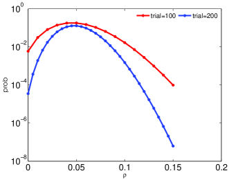
Fig  1: Probability of rejection fractions. The plot is the probability of $N\rho$ events rejected against the rejection fraction $\rho$ under the null hypothesis $H_{0}$ [Eq. (1)] and the significance level $0.05$. The red and blue lines are the case of $100$ trials and $200$ trials, respectively.

ACT pretreatment for neural data

In this section, we will elaborate the ACT pretreatment for neural data. As mentioned above, because of neural dynamics, the consecutive recording data points of neural activity are not statistically independent. However, high-dimensional two-sample test methods typically require statistically independent sampling to start with [24, 25, 26, 27, 28, 23]. For example of CQ method, the CQ statistic $Q_{n}\equiv T_{n}/\hat{\sigma}_{n}$, where $\hat{\sigma}_{n}$ is defined in Eq. (11) in Methods and

$$T_{n} = \frac{\sum_{i\neq j}^{n_{1}}\mathbf{X}_{1i}^{T}\mathbf{X}_{1j}}{n_{1}(n_{1}-1)}+\frac{\sum_{i\neq j}^{n_{2}}\mathbf{X}_{2i}^{T}\mathbf{X}_{2j}}{n_{2}(n_{2}-1)}-\frac{2\sum_{i=1}^{n_{1}}\sum_{j=1}^{n_{2}}\mathbf{X}_{1i}^{T}\mathbf{X}_{2j}}{n_{1}n_{2}},$$ (2)

$\mathbf{X}_{1}\in\mathbf{R}^{p\times n_{1}}$ and $\mathbf{X}_{2}\in\mathbf{R}^{p\times n_{2}}$ are the referential and the test samples, respectively, $p$ is the dimension size of samples, $n_{1}$ and $n_{2}$ are the sample sizes of the referential sample $\mathbf{X}_{1}$ and the test sample $\mathbf{X}_{2}$, respectively. Under the null hypothesis $H_{0}$, when the data points of $\mathbf{X}_{1}$ and $\mathbf{X}_{2}$ are sampled statistically independently, as $p$ tends to infinity, the statistic $Q_{n}$ would tend to the standard Gaussian distribution, by which the two-sample test can be performed. Under the null hypothesis $H_{0}$, it can be shown that the expected value $E(T_{n})=||\mu_{1}-\mu_{2}||_{2}^{2}$ is $0$, where $\mu_{1}$ and $\mu_{2}$ are means of the referential and the test samples, respectively. We consider a case that samples are dependent over time, such as $E(X_{k,j}X_{k,j+1})\neq E(X_{k,j})E(X_{k,j+1})$, where $k=1,2$, $X_{k,j}$ and $X_{k,j+1}$ are a pair of two consecutive sampling data points of $\mathbf{X}_{k}$, $E(x)$ denotes the expectation of stochastic variable $x$. Since $X_{k,j}X_{k,j+1}$ is a part of $T_{n}$ and $E(X_{k,j}X_{k,j+1})$ under dependent sampling deviates from $E(X_{k,j})E(X_{k,j+1})$ of independent sampling, as a result, $E(T_{n})$ would also have a deviation from $0$ even the null hypothesis $H_{0}$ holds. Since the expected value $E(T_{n})$ of the null hypothesis $H_{0}$ is $0$, the deviation of $E(T_{n})$ caused by dependent sampling cannot be dominated. Then, the distribution of $Q_{n}$ would deviate from the standard Gaussian distribution under the null hypothesis $H_{0}$. Hence, because of the bias induced by the correlation in samples over time, the CQ method is not applicable for dependent samples.

We observe that the correlation over dimensions would not affect $T_{n}$. To apply two-sample test methods in neural data, our idea is to transfer the correlation between data points over time into correlation over dimensions. For the case of one neuron, its spike train is recorded as a time series $(x_{1},x_{2},\cdots,x_{n})\in\{0,1\}^{n}$, where $n$ is the total recorded bins. If the correlation length of the time series is only one, i.e., $E(x_{i}x_{i+1})\neq E(x_{i})E(x_{i+1})$ and $E(x_{i}x_{i+j})=E(x_{i})E(x_{i+j})$ for $i\leq n-j$ and $j\geq 2$. We can turn the time series into a new two-dimensional series (Here, we assume $n$ is an even number. If $n$ is an odd number, we discard the last data point.)

$$Y=\left[\begin{array}[]{ccccc}x_{1}&x_{3}&\cdots&x_{n-3}&x_{n-1}\\ x_{2}&x_{4}&\cdots&x_{n-2}&x_{n}\end{array}\right],$$ (3)

in which every dimension of $Y$ is an independent series over time. In general, we don’t know the correlation length of a neural time series. Since the correlation time length of an aperiodic neural dynamical is usually around dozens of milliseconds, we can select a time window $\Delta T$ which is much larger than the neural correlation time length to partition the recording time. Multiple data points exist in every $\Delta T$ window. For example, if the sampling time bin size is $0.5\,\mathrm{ms}$ and $\Delta T=60\,\mathrm{ms}$, then, each $\Delta T$ window has $120$ data points. The mean value of these data points is calculated to represent each $\Delta T$ window. Since the correlation length of a neural time series is smaller than the selected $\Delta T$ , if two data points have time distance larger than $\Delta T$, they are effectively statistically independent. Hence, the correlation length of the new time series is only one. We can perform the same process as Eq. (3) to split every dimension into a two-dimensional series. If the original series has dimension $p$, the dimension of the new series is $2p$ as follows

$$\left[\begin{array}[]{ccccc}x_{11}&x_{13}&\cdots&x_{1,n-3}&x_{1,n-1}\\ x_{12}&x_{14}&\cdots&x_{1,n-2}&x_{1,n}\\ x_{21}&x_{23}&\cdots&x_{2,n-3}&x_{2,n-1}\\ x_{22}&x_{24}&\cdots&x_{2,n-2}&x_{2,n}\\ \vdots&\cdots&&\vdots&\vdots\end{array}\right].$$ (4)

We refer this process as the averaging and correlation transferring (ACT) method. Next, we would address the following problem of ACT:

(i) There are still some extra correlations, such as $x_{2}$ and $x_{3}$ in Eq. (3), which we refer to as antidiagonal correlation. In the estimator of the variance part of CQ statistic $Q_{n}$ [Eq. (11) in Methods], the antidiagonal correlation is not allowed, either. What is the influence of the antidiagonal correlation?

(ii) There are infinite values larger than the neural correlation length. How can we select a proper time window $\Delta T$?

We first use a numerical example to study the influence of different $\Delta T$. Fig. 2 displays a numerical example of scanning $\Delta T$ while applying ACT method to analyze data recorded from an I&F neural network. The network consists of $160$ excitatory and $40$ inhibitory neurons with random connections of probability $0.1$ driven by a Poisson input. Every trial requires $2\,\mathrm{s}$ recording time for each stimulus. The mean firing rate of each neuron is around $20\,\mathrm{Hz}$. We apply two-sample test methods for $400$ trials in four situations, namely, CQ with $200$ neurons (blue), CQ with $50$ neurons (black), TT with $200$ neurons (red) and TT with $50$ neurons (cyan). Note that the $50$ neurons are selected at random.

In Fig. 2a, the test stimulus is the same as the referential one. When $\Delta T$ is not too small (larger than $20\,\mathrm{ms}$), the rejection fractions of all cases are around the selected significance level $0.05$, which is consistent with the most probable outcome in Fig. 1. We can also examine whether the distribution of the statistic $Q_{n}$ tends to the standard Gaussian distribution. When $\Delta T$ is only $10\,\mathrm{ms}$, the distribution of $Q_{n}$ for the sample of $200$ neurons is far from the Gaussian distribution (Fig. 2c). When $\Delta T$ is larger, such as $60\,\mathrm{ms}$, the distribution of $Q_{n}$ for the sample of $200$ neurons fits the Gaussian distribution well (Fig. 2d). These phenomena indicate that the antidiagonal correlations barely have influence for a large $\Delta T$. There are two sources of antidiagonal correlation, one is the consecutive recordings of a neuron, such as $x_{12}$ and $x_{13}$ in Eq. (4), the other is the consecutive recordings of different neurons, such as $x_{22}$ and $x_{13}$ in Eq. (4). Here is the reason why the antidiagonal correlations barely have influence: (i) We select a $\Delta T$ larger than the correlation length of neuron data, then, the antidiagonal correlations from the consecutive recordings would be weak comparing to the variance; (ii) The correlation coefficient between neurons are normally rather weak ($\leq 0.1$) [33], then the antidiagonal correlations from the consecutive recordings of different neurons would also be rather weak comparing to the variance; (iii) In addition, for a data of dimension $p$, there are many non-zeros in the covariance of Eq. (4), i.e., $p$ variances of all dimensions and $p(p-1)$ pairwise correlations between dimensions. Therefore, the bias induced by antidiagonal correlations can be dominated. The correlations of neural data over time do not vanish, whereas ACT method split them into two parts, one is correlations between dimensions which can be dealt with by statistical methods, the other is antidiagonal correlations which can be dominated.

We also found that, when the test stimulus is different from the referential one, the rejection fraction of $H_{0}$ is not very sensitive to the parameter $\Delta T$ when $\Delta T$ is sufficiently large. The expectation of the statistic $Q_{n}$ [Eq. (9) in Methods] in CQ method is crucial to the rejection fraction. Hence, we study the expectation $E(Q_{n})$ for different $\Delta T$. We can compute the expectation $E(Q_{n})$ by Eq. (15) in Methods. We assume that $\Delta T$ is larger than the correlation time length of neural data and the total recording time is enough long. We denote $n$ as the sample size of both two samples with a time window $\Delta T$. When we use $\Delta T^{\prime}=\alpha\Delta T$, the new sample size is

$$n^{\prime}\approx n/\alpha.$$ (5)

Since the correlation between neurons is small comparing to the variance [33] and we have assumed that $\Delta T$ is larger than the correlation length of neuron data, we can assume the antidiagonal correlation is weak. Under this assumption, the covariance $\tilde{\Sigma}^{\prime}$ for $\Delta T^{\prime}$ and $\tilde{\Sigma}$ for $\Delta T$ (see Eq. (11) in Methods) have the following relation (See Appendix for a proof.)

$$\tilde{\Sigma}^{\prime}\approx\tilde{\Sigma}/\alpha,$$ (6)

then substituting Eqs. (5) and (6) into Eq. (15), we can obtain the expectation of $Q_{n}^{\prime}$ for $\Delta T^{\prime}$,

$$E(Q_{n}^{\prime})\approx 2C\frac{(n/\alpha)||\mu_{1}-\mu_{2}||^{2}}{\sqrt{tr(\tilde{\Sigma}^{2}/\alpha^{2})}}=2C\frac{n||\mu_{1}-\mu_{2}||^{2}}{\sqrt{tr(\tilde{\Sigma}^{2})}}=E(Q_{n}),$$

where the coefficient $C=1/(4\sqrt{2})$ as defined in Eq. (16) in Methods. Hence, $\Delta T$ would not affect the test result too much. But our recording time is finite, $\Delta T$ should not be selected as a too large value. Numerical simulations also show that the test result is not very sensitive to the parameter $\Delta T$. As is shown in Fig. 2b, where the test stimuli are $1.8\%$ larger in Poisson input magnitude than that of the referential stimuli, the rejection fractions of CQ and TT method do not change a lot when $\Delta T$ is not too small (larger than $40\,\mathrm{ms}$). We can also see that CQ have much higher rejection fractions than TT, and the results of CQ are better of $200$ neurons (blue dots) than those of $50$ neurons (black dots).

Since we have shown that the test result is not very sensitive to the parameter $\Delta T$, in the following, we will fix $\Delta T$ as $60\,\mathrm{ms}$ and show that this data pretreatment is applicable in most neural dynamical regimes.

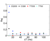
(a) Same

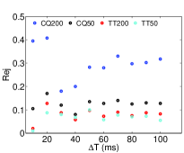
(b) Different

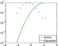
(c) $\Delta T=10\mathrm{ms}$

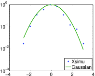
(d) $\Delta T=60\mathrm{ms}$

Fig  2: Test results for different time window $\Delta T$. The network consists of $160$ excitatory and $40$ inhibitory neurons with random connections with probability $0.1$ driven by a Poisson input. The coupling strength is $s=0.001\mathrm{ms^{-1}}$ (the corresponding excitatory/inhibitory postsynaptic potential is$\sim 0.1\mathrm{mV}$). The input parameters are chosen $\mu=0.7\,\mathrm{\mathrm{ms^{-1}}}$ (Poisson input rate) and $f=0.008\,\mathrm{\mathrm{ms^{-1}}}$ (Poisson input magnitude). The sampling time bin size is $0.5\,\mathrm{ms}$. Every trial requires $2\,\mathrm{s}$ recording for each stimulus. The mean firing rate is around $20\,\mathrm{Hz}$. We apply two-sample test methods for $400$ trials in four situations, CQ with $200$ neurons (blue), CQ with $50$ neurons (black), TT with $200$ neurons (red) and TT with $50$ neurons (cyan). For (a) and (b), the plot is the rejection fraction against the time window $\Delta T$. (a) The test stimuli are the same as the referential one. The dashed line is $y=0.05$. (b) The test stimuli are $1.8\%$ larger in Poisson input magnitude than the referential stimuli. (c) and (d) are the distributions of the statistic $Q_{n}$ for the case of $200$ neurons in (a) for $\Delta T=10\,\mathrm{ms}$ and $\Delta T=60\,\mathrm{ms}$, respectively. Blue dots are the numerical results and green lines are the standard Gaussian distributions, where both are normalized by the corresponding maximum values.

Numerical experiments on various neural dynamical regimes

Next, we examine whether this pretreatment is dependent of a particular dynamical regime. Dynamical regimes are often realized by a particular choice of network system parameters. We investigate this issue by scanning the magnitude $f$ and the rate $\mu$ in the Poisson drive of I&F neural networks. The scanned range of these parameters produces network dynamics with the range of firing rates ($3\,\mathrm{Hz}-50\,\mathrm{Hz}$) of real neurons. Note that there are typically three dynamical regimes for the I&F neurons with a fixed input magnitude $f$ [34]: (i) a highly fluctuating regime when the input rate $\mu$ is low; (ii) an intermediate regime when $\mu$ is moderately high; (iii) a low fluctuating or mean driven regime when $\mu$ is very high. The underlying network consists of $160$ excitatory and $40$ inhibitory neurons. It is a network of random connections with connection probability $0.1$ and the coupling strength between two connected neurons is selected at random based on the uniform distribution between $0$ and $1\mathrm{mV}$. Every trial requires $2\,\mathrm{s}$ recording time for each stimulus. We also apply two-sample test methods for $400$ trials in four situations, CQ with $200$ neurons (blue), CQ with $50$ neurons (black), TT with $200$ neurons (red) and TT with $50$ neurons (cyan). Note that the $50$ neurons are also selected at random. The parameters of stimuli of each index in Fig. 3a and b are from the left bottom corner of the box with the corresponding index inside in Fig. 3c. As is shown in Fig. 3a, CQ and TT both work well for all scanned dynamical regimes, i.e., the rejection fractions of the null hypotheses $H_{0}$ for the case of the same stimuli are around the selected significance level $0.05$. When the test stimuli are $1.8\%$ larger in Poisson input magnitude than those of the referential stimuli, Fig. 3b shows that CQ has higher rejection fractions than those of TT, and CQ with $200$ neurons has higher rejection fractions than those of CQ with $50$ neurons. Conclusion is that, in all scanned dynamical regimes, CQ method is better than TT method and CQ can use the advantage of large neuron number.

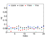
(a) Same

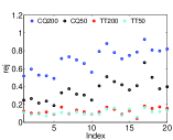
(b) Different

(c) Index

Fig  3: Test results in different dynamical regimes of an I&F neural network. The network consists of $160$ excitatory and $40$ inhibitory neurons with random connections with probability $0.1$ driven by Poisson inputs. The coupling strength between two connected neurons is selected at random based on the uniform distribution of the interval $[0,s]$, $s=0.01\mathrm{ms^{-1}}$ (the corresponding excitatory/inhibitory postsynaptic potential is$\sim 1\mathrm{mV}$). The Scanning parameters covers the realistic firing rates ($3\,\mathrm{Hz}-50\,\mathrm{Hz}$) of real neurons. The sampling time bin size is $0.5\,\mathrm{ms}$. $\Delta T$ is fixed as $60\,\mathrm{ms}$. The recording time at every trial for the referential and the test stimuli are $2\,\mathrm{s}$. We apply two-sample test methods for $400$ trials in four situations, CQ with $200$ neurons (blue), CQ with $50$ neurons (black), TT with $200$ neurons (red) and TT with $50$ neurons (cyan). For (a) and (b), the plot is the rejection fraction. (a) The test stimuli are the same as the referential one. (b) The test stimuli are $1.8\%$ larger in Poisson input magnitude than the referential stimuli. The parameters of stimuli of each index in (a) and (b) are from the left bottom corner of the box with the corresponding index inside in (c).

Swift discrimination tasks

As is shown in above numerical examples, every trial requires $2\,\mathrm{s}$ recording time for each stimulus. However, a prey can react to a predator in a shorter time, whereas it stays at a safe stimulus for a longer time. We can mimic the prey to perform a discrimination task. Thus, we can let the recording time of the referential stimulus $X_{1}$ longer, such as several seconds, and that of the test stimulus $X_{2}$ shorter, such as hundreds of milliseconds. There are usually two parts in a test statistic, one is the summation of difference of mean values [e.g. Eq. (10)], the other is the variance part [e.g. Eqs. (11), (12) and (13)], which is to normalize the statistic. The variance estimator usually requires more data points, for example, in our estimator for CQ statistic, the variance part requires at least $6$ data points (See Methods.), whereas the mean difference part requires at least $2$ data points. Since the recording time of $X_{1}$ is much longer than that of $X_{2}$, for CQ and TT methods, we can estimate the variance part by $X_{1}$ solely under the null hypothesis (See Methods.). We use a numerical example to show that this treatment is able to deal with swift discrimination of hundreds of milliseconds. Fig. 4 displays a swift discrimination version of Fig. 3. The recording time at every trial for $X_{1}$ and $X_{2}$ are $4\,\mathrm{s}$ and $360\,\mathrm{ms}$, respectively. In the case of the same stimuli, as is shown in Fig. 4a, the rejection fractions of TT and CQ are around the selected significance level $0.05$. This indicates TT and CQ are available to perform swift discrimination tasks. In the case of different stimuli, in which the test input is $1.5\%$ larger in Poisson input magnitude, the results are similar as above results, i.e., as is shown in Fig. 4b, CQ is better to discriminate different stimuli and CQ can use advantage of large neuron number.

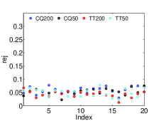
(a) Same

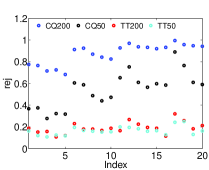
(b) Diff

Fig  4: Swift discrimination task. The recording time at every trial for $X_{1}$ and $X_{2}$ are $4\,\mathrm{s}$ and $360\,\mathrm{ms}$, respectively. Other parameters and illustrations are the same as Fig. 3. (a) The test stimuli are the same as the referential one. (b) The test stimuli are $1.5\%$ larger in Poisson input magnitude than the referential stimuli.

Tuning curve

Tuning curve is widely used to characterize the responses of one or a group of neurons with respect to various inputs. The width of a tuning curve is a popular way to potentially reflect the sensitivity of considered neurons to the inputs. In general, a tuning curve of firing rate is a classical and most used one. However, this idea is based on one classical viewpoint, in which neurons are considered to be independent. To understand how neurons code information, correlations between neurons need to be probed. There is an idea [32] considering pairwise correlations, which we refer to as Dependency in this paper (See Methods for details.). They consider the Kullback-Leibler distance of joint distribution of two selected neurons to the distribution of the forced-independent type, which is a type formed under the assumption that the neurons are acting independently.

To build a tuning curve by a two-sample test method, we establish a quantity from the rejection fraction,

$$N_{tst}=1-\rho,$$ (7)

where $\rho\in[0,1]$ is the rejection fraction as mentioned above, it is larger for the input of larger difference. The quantity $N_{tst}$ is also in $[0,1]$, but it is smaller for the input of larger difference.

To perform the comparison among different tuning curves, we record spike trains for drifting inputs of $10$ different orientations from an I&F neural network model of the primary visual cortex of the macaque (See Methods for Details.), as is shown in Fig. 5. For the tuning curves of the firing rate and the Dependency, we selected two neurons who have the same prefer orientations. The blue curves are normalized tuning curves of the firing rates for the two selected neurons, the black one is the normalized Dependency tuning curve of the two selected neurons. The red one is the normalized tuning curve of CQ method [Eq. (7)] using $2\,\mathrm{s}$ recording data for both the referential and test stimuli in each of $200$ trials, where the referential orientation is the prefer orientation of the two selected neurons in the method of Dependency. The cyan one is similar to the red one but using recording data of $4\,\mathrm{s}$. For the tuning curves of CQ method, we select about $340$ neurons to perform two-sample tests, where the firing rates of the selected neurons are larger than $2.5\,\mathrm{Hz}$ under at least referenntial inputs or test inputs. As is shown in Fig. 5, the curves of the CQ method are sharper than those of the other two methods, which indicates the CQ method is potentially better than other methods in discrimination tasks. The cyan curve is computed by CQ method with $4\,\mathrm{s}$ data for each trial, which is sharper than the red curve using $2\,\mathrm{s}$ data for each trial. This shows that the CQ method is able to use the advantage of large neural number and long recording time. It is no surprise that the CQ method is much better than other methods since we are able to use more information to estimate the turning curves.

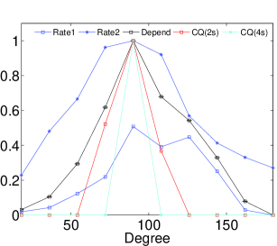
Fig  5: Normalized tuning curves in orientation tasks. We record spike trains for drifting inputs of $10$ different orientations from an I&F neural network model of the primary visual cortex of the macaque (See Methods for Details.). The sampling bin size is $0.5\,\mathrm{ms}$. For the tuning curves of the firing rate and the Dependency, we selected two neurons who have the same prefer orientations. The blue curves are normalized tuning curves of the firing rate for the two selected neurons, the black one is the normalized Dependency tuning curve of the two selected neurons. The red and cyan ones are normalized tuning curves of CQ method [Eq. (7)] using $2\,\mathrm{s}$ and $4\,\mathrm{s}$ data in each of $200$ trials, respectively, where the referential orientation is the prefer orientation of the two selected neurons in the method of Dependency. For tuning curves of CQ method, we select about $340$ neurons to perform two-sample tests, where the firing rates of the selected neurons are larger than $2.5\,\mathrm{Hz}$ at least under reference inputs or under test inputs. $\Delta T=60\,\mathrm{ms}$.

Discussion

To understand how neurons code stimulus in short time, a very first step is to detect the difference of external stimuli in the activities of neural networks. To achieve this goal, it requires proper high-dimensional methods for neural data of “large $p$, small $n$”. In another aspect, there is great progress in statistics to deal with samples of “large $p$, small $n$”. However, because of neural dynamics, the correlation of neural recordings over time forms a barrier between the neural data and high-dimensional statistical methods. ACT method, which transferring the correlation over time to the correlation over dimensions, shows a possible way to overcome this barrier. Through spike trains obtained from I&F neural networks, we show that ACT method enables the high-dimensional two-sample test methods to analyze numerical neural data within very short time (hundreds of milliseconds). Even there is only one trial data, with ACT method, we can also perform a two-sample test on neural data with single-trial statistical power.

Comparing to the TT method and other tuning curves considering only few neurons, based on ACT method, the high-dimensional statistical methods incorporating with neural correlations and neural number can probe finer difference in the activities of neural networks. How well the CQ method can use the advantage of large neuron number? As is shown in Eq. (17) in Methods, in an example of data of Gaussian distribution, since the covariance matrix is an identity, the expectation $E(Q_{n})$ is a linear function of $\sqrt{p}$, where $p$ is the dimension of the data. How is the situation in the neural data? Fig. 6 displays one case of Fig. 3, where $\mu=0.7\,\mathrm{\mathrm{ms^{-1}}}$ and $f=0.008\,\mathrm{\mathrm{ms^{-1}}}$, the expectation $E(Q_{n})$ is a nearly linear function of $\sqrt{p}$, where $p$ is the selected neuron number. This linear relation is a consequence of sparse covariance of neural data.

The antidiagonal correlation is a limitation of extending our method to data with slow decay dynamics. For the neural data, a $\Delta T$ of $60\,\mathrm{ms}$ also limits us from performing a two-sample test on data of $100\,\mathrm{ms}$ recording time.

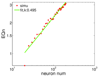
Fig  6: The relation between $\mathbf{E(Q_{n})}$ and neuron number. This is one case in Fig. 2, where $\mu=0.7\,\mathrm{\mathrm{ms^{-1}}}$ and $f=0.008\,\mathrm{\mathrm{ms^{-1}}}$. The red points are the $E(Q_{n})$ from numerical neural data with respect to the number of selected neurons, and the green line is a linear fitting in the log-log plot with slope $0.495$. This shows that $E(Q_{n})$ is a nearly linear function of $\sqrt{p}$, where $p$ is neuron number.

Methods

High-dimensional two-sample test problem

In general, we can describe the problem in the following way. $\mathbf{X}_{k1}$,$\mathbf{X}_{k2}$,$\cdots$,$\mathbf{X}_{kn_{k}}$$\in$$R^{p\times 1}$ are a sample of data sampled independently from the $k$-th distribution, where $k=1,2$, $p$ is the dimension and $n_{k}$ is the sample size of the $k$-th sample. The mean value and covariance of the $k$-th sample are denoted by $\mathbf{\mathbf{\mathbf{\mu}}}_{k}=(\mu_{k1},\mu_{k2},\cdots,\mu_{kp})^{T}\in R^{p\times 1}$ and $\Sigma_{k}\in R^{p\times p}$, respectively. The null and alternative hypotheses are as follows:

$$H_{0}:\mu_{1}=\mu_{2}\quad v.s.\quad H_{1}:\mu_{1}\neq\mu_{2},$$ (8)

where the null hypothesis $H_{0}$ consists of $p$ marginal hypotheses, i.e., $H_{0l}:\mu_{1l}=\mu_{2l}$, for $l=1,\cdots,p$. If any component of $\mu_{1}$ is not equal to the corresponding one of $\mu_{2}$, $H_{0}$ is rejected. The significance level for this paper is selected as $0.05$.

CQ two-sample Test

The CQ method [23] considers the test statistic $Q_{n}$ as follows, under the null hypothesis,

$$Q_{n}\triangleq\frac{T_{n}}{\hat{\sigma}_{n}}\overset{d}{\rightarrow}N(0,1)\qquad p\rightarrow\infty,n\rightarrow\infty,$$ (9)

where $\overset{d}{\rightarrow}$ indicates that the distribution of $Q_{n}$ converges to the standard Gaussian distribution in distribution, $T_{n}$ and $\hat{\sigma}_{n}$ are defined as below,

$$T_{n} = \frac{\sum_{i\neq j}^{n_{1}}\mathbf{X}_{1i}^{T}\mathbf{X}_{1j}}{n_{1}(n_{1}-1)}+\frac{\sum_{i\neq j}^{n_{2}}\mathbf{X}_{2i}^{T}\mathbf{X}_{2j}}{n_{2}(n_{2}-1)}-\frac{2\sum_{i=1}^{n_{1}}\sum_{j=1}^{n_{2}}\mathbf{X}_{1i}^{T}\mathbf{X}_{2j}}{n_{1}n_{2}},$$ (10)

$$\hat{\sigma}_{n1}^{2}=\frac{2\widehat{tr(\Sigma_{1}^{2})}}{n_{1}(n_{1}-1)}+\frac{2\widehat{tr(\Sigma_{2}^{2})}}{n_{2}(n_{2}-1)}+\frac{4\widehat{tr(\Sigma_{1}\Sigma_{2})}}{n_{1}n_{2}},$$ (11)

in which $\hat{\sigma}_{n}$ is the standard deviation of $T_{n}$, $\Sigma_{k}$ is the covariance of $\mathbf{X}_{2}$. We use the following estimators for $\widehat{tr(\Sigma_{i}^{2})}$ and $\widehat{tr(\Sigma_{1}\Sigma_{2})}$, which are slightly different with the estimators in Ref. [23]. We denote $A^{jk}$ is a copy of $X_{1}$ eliminating the $j$-th and the $k$-th data point,

$$\widehat{tr(\Sigma_{1}^{2})}_{\mathrm{new}}=\{n_{1}(n_{1}-1)\}^{-1}tr\{\sum_{j\neq k}^{n_{1}}(\mathbf{X}_{1j}-\mathbf{c}_{11}^{jk})(\mathbf{X}_{1j}-\mathbf{c}_{12}^{jk})^{T}(\mathbf{X}_{1k}-\mathbf{c}_{13}^{jk})(\mathbf{X}_{1k}-\mathbf{c}_{14}^{jk})^{T}\},$$ (12)

where $\mathbf{c}_{1i}^{jk}$, $i=1,2,3,4$, is the sample mean of the $i$-th quarter of $A^{jk}$. We denote $A^{l}$ is a copy of $X_{1}$ eliminating the $l$-th sample and $B^{k}$ as a copy of $X_{2}$ eliminating the $k$-th sample,

$$\widehat{tr(\Sigma_{1}\Sigma_{2})}_{\mathrm{new}}=\{n_{1}n_{2}\}^{-1}tr\{\sum_{l}^{n_{1}}\sum_{k}^{n_{2}}(\mathbf{X}_{1l}-\mathbf{d}_{11}^{l})(\mathbf{X}_{1l}-\mathbf{d}_{12}^{l})^{T}(\mathbf{X}_{2k}-\mathbf{d}_{21}^{k})(\mathbf{X}_{2k}-\mathbf{d}_{22}^{k})^{T}\},$$ (13)

where $\mathbf{d}_{1i}^{l}$, $i=1,2$ is the sample mean of the $i$-th half of $A^{l}$, $\mathbf{d}_{2i}^{k}$, $i=1,2$ is the sample mean of the $i$-th half of $B^{k}$.

Elementary derivations show that

$$E(T_{n})=||\mu_{1}-\mu_{2}||^{2},$$ (14)

where $E(x)$ is the expectation of a stochastic variable $x$, $E(X_{ki})=\mu_{k}$ for $k=1,2$ and $1\leq i\leq n_{k}$.

The expectation of $Q_{n}$ is

$$E(Q_{n})=C\frac{n_{0}||\mu_{1}-\mu_{2}||^{2}}{\sqrt{tr(\tilde{\Sigma}^{2})}},$$ (15)

where $n_{0}=n_{1}+n_{2}-2$, the composite covariance $\tilde{\Sigma}=(1-h)\Sigma_{1}+h\Sigma_{2}$, $h=n_{1}/(n_{1}+n_{2})$ and

$$C=\frac{h(1-h)}{\sqrt{2}}.$$ (16)

To see the power of CQ method intuitively, we give a simple example. Both samples have the same lengths, denoted as $n$, and the same dimensions, denoted as $p$. The mean of the first sample is $\mu_{1}=0_{1\times p}$, and that of the second sample is $\mu_{2}=1_{1\times p}$. Assuming that the $k$-th sample ($k=1,2$) is sampled independently from the normal distribution $N(\mu_{k},1)$, then, we have

$$E(Q_{n})\approx\frac{n||\mu_{1}-\mu_{2}||^{2}}{\sqrt{8tr(\Sigma^{2})}}=n\sqrt{p}/\sqrt{8}.$$ (17)

Since the expectation of $Q_{n}$ is crucial to the resolution of the method, $p$ and $n$ are therefore important factors to the resolution.

In a swift two-sample test, the variance part is estimated by $X_{1}$ solely. Eq. (11) would become

$$\hat{\sigma}_{n1}^{2}=\frac{2\widehat{tr(\Sigma_{1}^{2})}}{n_{1}(n_{1}-1)}+\frac{2\widehat{tr(\Sigma_{1}^{2})}}{n_{2}(n_{2}-1)}+\frac{4\widehat{tr(\Sigma_{1}^{2})}}{n_{1}n_{2}},$$

where $\widehat{tr(\Sigma_{1}^{2})}$ is estimated by Eq. (12).

Student t-test (TT)

$\mathbf{x}=(x_{1},\cdots,x_{n_{x}})$ and $\mathbf{y}=(y_{1},\cdots,y_{n_{y}})$ are independently sampled from two one-dimensional distributions for $n_{x}$ and $n_{y}$ times, respectively. The statistic quantity of Student t-test (TT) test is defined as follows:

$$Q_{n}^{TT}\triangleq\frac{\overline{x}-\overline{y}}{\sqrt{\frac{s_{x}^{2}}{n_{x}}+\frac{s_{y}^{2}}{n_{y}}}},$$ (18)

where

$$\overline{x}=\frac{1}{n_{x}}\sum_{j=1}^{n_{x}}x_{j},$$ (19)

$$\overline{y}=\frac{1}{n_{y}}\sum_{j=1}^{n_{y}}y_{j},$$ (20)

$$s_{x}^{2}=\frac{1}{n_{x}-1}\sum_{j=1}^{n_{x}}(x_{j}-\overline{x})^{2},$$ (21)

$$s_{y}^{2}=\frac{1}{n_{y}-1}\sum_{j=1}^{n_{y}}(y_{j}-\overline{y})^{2}.$$ (22)

For data with dimension $p,$ it can be dealt with by TT one by one dimension independently. In order to keep the total significance level still being $0.05$, the significance level for each dimension is selected by $0.05/p$. For each dimension, the acceptation of null hypothesis is $1-0.05/p$. If we assume that data of different dimensions are independent, for a large $p$, the acceptation of null hypothesis of total test is

$$(1-\frac{0.05}{p})^{p}\approx 1-0.05,$$

which indicates the significance level for the whole test is still around $0.05$.

In a swift two-sample test, the variance part is estimated by $x$ solely, i.e., $s_{y}^{2}$ is replaced by $s_{x}^{2}$ in the $Q_{n}^{TT}$ in Eq. (18).

Integrate-and-fire model

In this paper, we use the integrate-and-fire (I&F for short) neuron model for neural simulations. The dynamics of conductance-based I&F model [35] is governed by

$$\begin{cases}\frac{dV_{i,Q}}{dt}&=-G^{L}(V_{i,Q}-\epsilon^{L})-G_{i,Q}^{E}(V_{i,Q}-\epsilon^{E})-G_{i,Q}^{I}(V_{i,Q}-\epsilon^{I}),\\ \frac{dG_{i,Q}^{E}}{dt}&=-\frac{G_{i,Q}^{E}}{\sigma^{E}}+S_{QE}\sum_{j_{E}\neq i}^{N_{E}}\sum_{k}m_{ij_{E}}\delta(t-T_{j_{E},k})+f_{E}\sum_{l}\delta(t-T_{i,l}^{F,E})\\ \frac{dG_{i,Q}^{I}}{dt}&=-\frac{G_{i,Q}}{\sigma^{I}}+S_{QI}\sum_{j\neq i}^{N_{I}}\sum_{k}m_{ij_{I}}\delta(t-T_{j_{I},k})+f_{I}\sum_{l}\delta(t-T_{i,l}^{F,I}),\end{cases},$$ (23)

where the $i$-th neuron with type $Q=E$ or $I$, has both excitatory conductance $G_{i,Q}^{E}$ and inhibitory conductance $G_{i,Q}^{I}$, and the $\epsilon^{E}$ and $\epsilon^{I}$ are the excitatory and inhibitory reversal potentials, respectively. $V_{i,Q}$ is the membrane potential. $G^{L}$ is the leak conductance. The decay time scale of excitatory and inhibitory synaptic conductance are $\sigma^{E}$ and $\sigma^{I}$, respectively. $S_{QE}$ and $S_{QI}$ are the strength of input from excitatory and inhibitory neurons in the system, respectively. We only use excitatory Poisson input to drive the system with the rate $\mu$ and magnitude $f_{E}=f$, $f_{I}=0$. The network structure is denoted by adjacency matrix $m_{ij}$.

The $i$-th neuron will evolve according to Eq. (23) until $V_{i,Q}$ reaches the voltage threshold $V_{T}$ at which the neuron will produce a spike. The spike time is denoted by $T_{i,k}^{F,Q}$, where $i$ is the index of neuron, $k$ is the order of the spike of neuron $i$. Then $V_{i,Q}$ is reset to be the resting potential $V_{R}$ immediately. $V_{i,Q}$ will be kept at $V_{R}$ for a refractory period $\tau_{ref}$ . When this is over, $V_{i,Q}$ starts to evolve again.

The parameter set we used in the numerical experiment is: $\tau_{\mathrm{ref}}=2\,\mathrm{ms}$, $\sigma^{E}=2\,\mathrm{ms}$, $\sigma^{I}=5\,\mathrm{ms}$, $G^{L}=0.05\,\mathrm{ms^{-1}}$. The voltage uses a normalized unit: $V_{T}=1$, $V_{R}=0$, $\epsilon^{L}=0$, $\epsilon^{E}=14/3$, $\epsilon^{I}=-2/3$. They correspond to typical physiological values: $G^{L}=50\times 10^{-6}\,\mathrm{\Omega^{-1}cm^{-2}}$, $V_{T}=-55\,\mathrm{mV}$, $V_{R}=\epsilon^{L}=-70\,\mathrm{mV}$, $\epsilon^{I}=-80\,\mathrm{mV}$, $\epsilon^{E}=0\,\mathrm{mV}$. We choose this set of parameters because they are widely used.

Neural network model of the primary visual cortex of the macaque

The simulation model of orientation discrimination task is an I&F neural network model of the primary visual cortex (V1) of the macaque, details can be found at references [36, 37]. In this paper, the network model consists of $4096$ neurons, $25\%$ inhibitory neurons. Each V1 cell sees a collection of Lateral geniculate nucleus (LGN) neurons, where the number of LGN neurons is uniform selected from $0$ to $30$. The on and off cells confer the orientation and spatial phase preference of V1 cell. Orientation preference is laid out in pinwheels. The V1 neurons also get inhibitory and excitatory input from other V1 cells. The input is drifting sinusoid,

$$I(\vec{x},t)=I_{0}[1+\epsilon\sin(\omega t-\vec{k}\cdot\vec{x}+\phi)],$$

where intensity $I_{0}=15.0$, contrast $\epsilon=100\%$, temporal frequency $\omega=2\pi\text{$\times$}20\,\mathrm{Hz}$, and spatial phase $\phi$ depends on the neural location. The spatial frequency wave vector of the grating, $\vec{k}=k(\cos\theta,\sin\theta)$, has spatial frequency $k=2\pi\text{$\times$}76.9\,\mathrm{\text{/cycle}}$ and orientation $\theta$. In the task, we pick an orientation input as the referential stimuli, then, we can compute the rejection fraction of a test orientation input by a two-sample test method.

Tuning curve: Dependency

Another tuning curve [32] considers a pair of neurons, which we refer to as Dependency. It considers the Kullback-Leibler distance between joint distribution of two selected neurons and the distribution of its forced-independent type, which is a type formed under the assumption that the neurons are acting independently. By denoting $P_{\sigma_{i}\sigma_{j}}$ is the probability of neuron state $(\sigma_{i},\sigma_{j})$, the marginal distribution of first neuron can be obtained by

$$p_{1}^{1}=P_{10}+P_{11},$$

$$p_{0}^{1}=P_{01}+P_{00},$$

where $p_{\sigma}^{1}$ denotes the probability of the first neuron with state $\sigma\in\{0,1\}$ of first neuron. Similarly, $p_{\sigma}^{2}$ can be evaluated. By assuming that neurons are independent, the joint distribution of forced-independent type $Q_{\sigma_{i},\sigma_{j}}$ can be obtained,

$$Q_{11}=p_{1}^{1}\times p_{1}^{2},$$

$$Q_{10}=p_{1}^{1}\times p_{0}^{2},$$

$Q_{01}$, $Q_{00}$ can be evaluated similarly. The Dependency is defined as following,

$$D=\sum_{\sigma_{i},\sigma_{j}\in\{0,1\}}P_{\sigma_{i},\sigma_{j}}\log\frac{P_{\sigma_{i},\sigma_{j}}}{Q_{\sigma_{i},\sigma_{j}}}.$$

Appendix

The relation between $\Sigma^{\prime}$ and $\Sigma$

In ACT method, the time window $\Delta T$ is a free parameter. Nevertheless, we show that the test result is not sensitive to the parameter $\Delta T$ when $\Delta T$ is larger than correlation length. To show this, we prove an important relation Eq. (6), which is a consequence under the condition that the antidiagonal correlation is very weak. For the sake of illustration, we consider a two-dimensional time series,

$$\left(\begin{array}[]{c}\mathbf{u}\\ \mathbf{v}\end{array}\right)=\left(\begin{array}[]{ccccc}u_{1}&u_{2}&\cdots&u_{i}&\cdots\\ v_{1}&v_{2}&\cdots&v_{i}&\cdots\end{array}\right),$$

where each dimension is an independent time series, the covariance is denoted as

$$\Sigma=\left(\begin{array}[]{cc}\sigma_{u}^{2}&\sigma_{uv}^{2}\\ \sigma_{uv}^{2}&\sigma_{v}^{2}\end{array}\right).$$

If we select another $\Delta T^{\prime}=\alpha\Delta T$, for the sake of simplicity, we assume that $\alpha$ is an integer, then, we have another two-dimensional time series,

$$\left(\begin{array}[]{c}\mathbf{U}\\ \mathbf{V}\end{array}\right)=\left(\begin{array}[]{ccccc}U_{1}&U_{2}&\cdots&U_{i}&\cdots\\ V_{1}&V_{2}&\cdots&V_{i}&\cdots\end{array}\right),$$

where

$$U_{i}=\frac{1}{\alpha}\sum_{j=1}^{\alpha}u_{(i-1)\alpha+j},$$

$$V_{i}=\frac{1}{\alpha}\sum_{j=1}^{\alpha}v_{(i-1)\alpha+j}.$$

We denote the covariance of new time series as

$$\Sigma^{\prime}=\left(\begin{array}[]{cc}\sigma_{U}^{2}&\sigma_{UV}^{2}\\ \sigma_{UV}^{2}&\sigma_{V}^{2}\end{array}\right).$$

The variance of $\mathbf{U}$ is

$$\sigma_{U}^{2}=\mbox{var}(\frac{1}{\alpha}\sum_{j=1}^{\alpha}u_{j})=\frac{1}{\alpha}\sigma_{u}^{2}.$$ (24)

The variance of $\mathbf{V}$ is

$$\sigma_{V}^{2}=\mbox{var}(\frac{1}{\alpha}\sum_{j=1}^{\alpha}v_{j})=\frac{1}{\alpha}\sigma_{v}^{2}.$$ (25)

The covariance of $\mathbf{U}$ and $\mathbf{V}$ is

$$\sigma_{UV}^{2} = \mbox{$E$}[\frac{1}{\alpha}\sum_{i=1}^{\alpha}u_{i}-\mbox{$E$}(\frac{1}{\alpha}\sum_{j=1}^{\alpha}u_{j})][\frac{1}{\alpha}\sum_{i=1}^{\alpha}v_{i}-\mbox{E}(\frac{1}{\alpha}\sum_{j=1}^{\alpha}v_{j})]$$

$$= \mbox{$E$}(\frac{1}{\alpha}\sum_{i=1}^{\alpha}u_{i}\cdot\frac{1}{\alpha}\sum_{j=1}^{\alpha}v_{j})-Eu_{1}Ev_{1}$$

$$= \frac{1}{\alpha^{2}}\sum_{i,j=1}^{\alpha}E(u_{i}v_{j})-Eu_{1}Ev_{1},$$

where $E(x)$ denotes the expectation of a stochastic variable $x$. We have a key assumption that the antidiagonal correlation is very weak, i.e.,

$$E(u_{i}v_{j})\approx Eu_{i}Ev_{j},\quad i\neq j.$$ (26)

Based on the assumption Eq. (26), we have

$$\sigma_{UV}^{2} = \frac{1}{\alpha^{2}}\sum_{i=1}^{\alpha}E(u_{i}v_{i})+\frac{1}{\alpha^{2}}\sum_{i\neq j}^{\alpha}E(u_{i}v_{j})-Eu_{1}Ev_{1}$$

$$\approx \frac{1}{\alpha}E(u_{1}v_{1})+\frac{\alpha(\alpha-1)}{\alpha^{2}}Eu_{1}Ev_{1}-Eu_{1}\mbox{E}v_{1}$$

$$= \frac{1}{\alpha}(E(u_{1}v_{1})-Eu_{1}Ev_{1}),$$

therefore,

$$\sigma_{UV}^{2}\approx\frac{1}{\alpha}\sigma_{uv}^{2}.$$ (27)

From Eqs. (24,25,27), we arrive at

$$\Sigma^{\prime}\approx\frac{1}{\alpha}\Sigma.$$ (28)

Since the covariance is a relation of every two dimensions, Eq. (28) can be generalized to high-dimensional time series. The assumption Eq. (26) is based on two facts, one is that the correlation between neurons is small comparing to the variance [33], the other is that we select a $\Delta T$ which is larger than the correlation length of neuron data. Since no matter for $\Delta T$ or $\Delta T^{\prime}$, data processing is based on the original sampled data, therefore, $\alpha$ does not have to be an integer.

References

- 1. Chittka L, Skorupski P, Raine NE. Speed–accuracy tradeoffs in animal decision making. Trends in Ecology & Evolution. 2009;24(7):400–407.
- 2. Uchida N, Kepecs A, Mainen ZF. Seeing at a glance, smelling in a whiff: rapid forms of perceptual decision making. Nature Reviews Neuroscience. 2006;7(6):485–491.
- 3. Mainen ZF. Behavioral analysis of olfactory coding and computation in rodents. Current opinion in neurobiology. 2006;16(4):429–434.
- 4. Abraham NM, Spors H, Carleton A, Margrie TW, Kuner T, Schaefer AT. Maintaining accuracy at the expense of speed: stimulus similarity defines odor discrimination time in mice. Neuron. 2004;44(5):865–876.
- 5. Rousselet GA, Macé MJM, Fabre-Thorpe M. Is it an animal? Is it a human face? Fast processing in upright and inverted natural scenes. Journal of vision. 2003;3(6):5.
- 6. Roitman JD, Shadlen MN. Response of neurons in the lateral intraparietal area during a combined visual discrimination reaction time task. The Journal of neuroscience. 2002;22(21):9475–9489.
- 7. Zandvakili A, Kohn A. Coordinated Neuronal Activity Enhances Corticocortical Communication. Neuron. 2015;87(4):827–839.
- 8. Harris AZ, Gordon JA. Long-Range Neural Synchrony in Behavior. Annual review of neuroscience. 2015;(0).
- 9. Schneidman E, Berry MJ, Segev R, Bialek W. Weak pairwise correlations imply strongly correlated network states in a neural population. Nature. 2006;440(7087):1007–1012.
- 10. Shlens J, Field GD, Gauthier JL, Grivich MI, Petrusca D, Sher A, et al. The structure of multi-neuron firing patterns in primate retina. The Journal of neuroscience. 2006;26(32):8254–8266.
- 11. Brown EN, Kass RE, Mitra PP. Multiple neural spike train data analysis: state-of-the-art and future challenges. Nature neuroscience. 2004;7(5):456–461.
- 12. Buzsáki G. Large-scale recording of neuronal ensembles. Nature neuroscience. 2004;7(5):446–451.
- 13. Chapin JK. Using multi-neuron population recordings for neural prosthetics. Nature neuroscience. 2004;7(5):452–455.
- 14. Buzsáki G, Anastassiou CA, Koch C. The origin of extracellular fields and currents-EEG, ECoG, LFP and spikes. Nature reviews neuroscience. 2012;13(6):407–420.
- 15. Shimazaki H, Amari Si, Brown EN, Grün S. State-space analysis of time-varying higher-order spike correlation for multiple neural spike train data. PLoS computational biology. 2012;8(3):e1002385.
- 16. Trousdale J, Hu Y, Shea-Brown E, Josic K. Impact of network structure and cellular response on spike time correlations. PLoS Comput Biol. 2012;8(3):e1002408–e1002408.
- 17. Cunningham JP, Byron MY. Dimensionality reduction for large-scale neural recordings. Nature neuroscience. 2014;.
- 18. Bernyi A, Somogyvari Z, Nagy AJ, Roux L, Long JD, Fujisawa S, et al. Large-scale, high-density (up to 512 channels) recording of local circuits in behaving animals. Journal of neurophysiology. 2014;111(5):1132–1149.
- 19. Khodagholy D, Gelinas JN, Thesen T, Doyle W, Devinsky O, Malliaras GG, et al. NeuroGrid: recording action potentials from the surface of the brain. Nature neuroscience. 2015;18(2):310–315.
- 20. Xu ZQJ, Bi G, Zhou D, Cai D. A dynamical state underlying the second order maximum entropy principle in neuronal networks. Communications in Mathematical Sciences. 2017;15(3):665–692.
- 21. Xu ZQJ, Zhou D, Cai D. Dynamical and Coupling Structure of Pulse-Coupled Networks in Maximum Entropy Analysis. arXiv preprint arXiv:180804499. 2018;.
- 22. Xu ZQJ, Crodelle J, Zhou D, Cai D. Maximum Entropy Principle Analysis in Network Systems with Short-time Recordings. arXiv preprint arXiv:180810506. 2018;.
- 23. Chen SX, Qin YL, et al. A two-sample test for high-dimensional data with applications to gene-set testing. The Annals of Statistics. 2010;38(2):808–835.
- 24. Srivastava MS, Du M. A test for the mean vector with fewer observations than the dimension. Journal of Multivariate Analysis. 2008;99(3):386–402.
- 25. Lopes M, Jacob L, Wainwright MJ. A more powerful two-sample test in high dimensions using random projection. In: Advances in Neural Information Processing Systems; 2011. p. 1206–1214.
- 26. Gretton A, Borgwardt KM, Rasch MJ, Schölkopf B, Smola A. A kernel two-sample test. The Journal of Machine Learning Research. 2012;13(1):723–773.
- 27. Tony Cai T, Liu W, Xia Y. Two-sample test of high dimensional means under dependence. Journal of the Royal Statistical Society: Series B (Statistical Methodology). 2014;76(2):349–372.
- 28. Reddi SJ, Ramdas A, Póczos B, Singh A, Wasserman LA. On the High Dimensional Power of a Linear-Time Two Sample Test under Mean-shift Alternatives. In: AISTATS; 2015. .
- 29. Fan J, Han F, Liu H. Challenges of big data analysis. National science review. 2014;1(2):293–314.
- 30. Han F, Liu H. Principal Component Analysis on non-Gaussian Dependent Data. In: ICML (1); 2013. p. 240–248.
- 31. Rauch A, La Camera G, Lüscher HR, Senn W, Fusi S. Neocortical pyramidal cells respond as integrate-and-fire neurons to in vivo–like input currents. Journal of neurophysiology. 2003;90(3):1598–1612.
- 32. Samonds JM, Allison JD, Brown HA, Bonds A. Cooperation between area 17 neuron pairs enhances fine discrimination of orientation. The Journal of neuroscience. 2003;23(6):2416–2425.
- 33. Cohen MR, Kohn A. Measuring and interpreting neuronal correlations. Nature Neuroscience. 2011;14(7):811–819.
- 34. Zhou D, Xiao Y, Zhang Y, Xu Z, Cai D. Granger causality network reconstruction of conductance-based integrate-and-fire neuronal systems. PloS one. 2014;9(2):e87636.
- 35. Gerstner W, Kistler WM. Spiking neuron models: Single neurons, populations, plasticity. Cambridge university press; 2002.
- 36. Tao L, Shelley M, McLaughlin D, Shapley R. An egalitarian network model for the emergence of simple and complex cells in visual cortex. Proceedings of the National Academy of Sciences. 2004;101(1):366–371.
- 37. Tao L, Cai D, McLaughlin DW, Shelley MJ, Shapley R. Orientation selectivity in visual cortex by fluctuation-controlled criticality. Proceedings of the National Academy of Sciences. 2006;103(34):12911–12916.