L1 Stream Deflection and Ballistic Launching at the Disk Bow Shock: An Absorption-line Velocity Analysis in Semi-Detached Binaries

Abstract

Observations of semi-detached interacting binaries reveal orbital modulation in the optical, UV, and X-ray bands, indicating the presence of absorbing material obscuring the disk and accreting primary star at specific orbital phases consistent with $L1$ stream material overflowing the disk edge.

We simulate the L1 stream interaction with the disk using tests particles within the context of the Roche model in the restricted three-body problem. At the disk bow shock the L1 stream particles are deflected and launched onto ballistic trajectories above the disk (as would normally occurs at the front of a detached shock in a hypersonic flow past a blunt body). At a given scale height, the material is assumed to continue without being affected by the disk, while at lower altitude it is being launched at an increasing elevation, as well as gradually being dragged by the Keplerian flow. Near the disk mid-plane ($z<<H$) the material is assumed to become part of the disk. We follow the stream material ballistic trajectories over the disk surface, where they reach a maximum height $z/r$ at a binary phase $\Phi\sim 0.75$, and land onto the disk at a smaller radius around phase $\Phi\sim 0.5$. The phase of the maximum height, phase of the landing site and phase of the hot spot itself, all decrease significantly with decreasing disk radius.

The radial velocity for each $L1$ stream ballistic trajectory along the line of sight (of the observer) to the hot inner parts of the disk is computed as a function of the orbital phase for a binary configuration matching the dwarf nova U Geminorum. The computed velocity amplitudes, phases, and pattern match the observed velocity offsets of the metal lines in the FUSE spectrum of U Gem during outburst. As ballistic trajectories are much easier to compute than realistic three-dimensional hydrodynamical simulations, we propose the use of the $L1$ stream deflection and ballistic launching as a means for the analysis of the absorption-line orbital variability in semi-detached binaries and to assess or confirm, with some limitations, system parameters such as the mass ratio, inclination, and disk outer radius.

Accepted version 1.0in

1 Introduction

Semi-detached interacting binaries are systems in which one star, the donor (or secondary), fills its Roche lobe and loses matter to the other star, the accretor (or primary). In most cases, the matter forms a disk around the primary, and as it is being accreted (either sporadically, periodically, or continuously), highly energetic emission is released. The accreting star can be either a main-sequence star (e.g. such as in Algol variables), a white dwarf (as in cataclysmic variables - CVs), or even a neutron star or a black hole (as in low-mass x-ray binaries - LMXBs). Semi-detached binaries have been extensively studied and analyzed for many decades now, and they have become the favorite objects to observe for the study of accretion disks (Nussbaumer & Orr, 1994).

In these systems, the secondary reaches its Roche limit and, consequently, funnels matter through the first Lagrangian point ($L1$) into the Roche lobe of the primary (Kuiper, 1941; Kruszewski, 1966; Prendergast & Taam, 1974). After the stream of matter leaves the $L1$ vicinity, it sets onto a ballistic trajectory around the primary, and then collides with itself to form a ring of matter (Lubow & Shu, 1975), which eventually grows into an accretion disk (e.g. Murray, 1991). The incoming $L1$ stream continues to interact with the accretion disk after its formation by impacting its edge to form a “hot spot” on the rim of the disk, which appears as an orbital modulation in the light curve that cannot be attributed to primary or secondary eclipses. For example, Krzeminski (1965) showed that the optical light curve of the dwarf nova U Geminorum (a CV) exhibits eclipses in quiescence (low mass accretion rate), which occur earlier during rise to outburst, and return to their original phase as the systems fades back into quiescence. These can be explained as eclipses of the hot spot by the secondary star, shifting phase as the hot spot moves along the rim of the disk which expands during rise to outburst and shrinks during decline.

However, a second hot spot often appears on the surface of the disk (in Doppler tomograms; Marsh, 1985; Marsh & Horne, 1988), which is due (as first demonstrated by Lubow (1989)) to the $L1$ stream material flowing over the disk edge and impacting the disk at smaller radii. Theoretically, one can differentiate between two cases of stream overflow. In the first case (Lubow & Shu, 1975, 1976; Lubow, 1989), parts of the $L1$ stream is high enough above the disk (i.e. where the stream is much denser than the disk) to continue on a ballistic trajectory unaffected by the disk edge, and impacts the disk near the closest approach radius ($\varpi_{\rm min}$ in Lubow & Shu (1975)) at phase $\Phi\approx 0.6$. In the second case, as shown with the advance of three-dimensional hydrodynamical simulations (e.g. Armitage & Livio, 1996; Blondin, 1998; Kunze et al., 2001; Bisikalo et al., 2000, 2003), the $L1$ stream material is deflected vertically from the impinging region (i.e. at the first hot spot) and flies in a more or less diffuse stream to inner parts of the disk, hitting the disk surface close to the circularization radius ($\varpi_{\rm d}$ in Lubow & Shu (1975)) at orbital phase $\Phi=0.5$.

The vertical deflection of stream matter at the (first) hot spot can itself be due to either deflection by the bow shock itself (Kunze et al., 2001, similar to the isothermal case in Armitage & Livio (1998)), or due to high pressure of the hot post-shock expanding gas out of hydrostatic balance in the hot spot region (Kunze et al., 2001, similar to the adiabatic case of Armitage & Livio (1998), and as observed in WZ Sge by Spruit & Rutten (1998)).

These 3D simulations of the stream overflowing the disk have been able to explain the veiling of the accreting star in X-ray observations of CVs and LMXBs around orbital phase $\Phi=0.7$, when the inclination is at least $65^{\circ}$ (Kunze, Speith, & Hessman, 2001), and can even explain jets perpendicular to the orbital plane as observed in Algol-type binaries.

The complexity of the stream-disk interaction and how this affects the observations depend on the system parameters (e.g. such as inclination, binary mass ratio) and the state of the system (high mass transfer rate versus low mass transfer rate). Whether parts of the stream overflow the disk in a ballistic trajectory also depends on the parameters such as the disk radius or whether the disk and stream are aligned (tilted disks would certainly facilitates ballistic stream overflow as the stream may miss the disk). Also, if the material gains energy, e.g. is accelerated by the disk Keplerian flow, then it could be ejected or launched into a circumbinary orbit. It follows that for each system a slightly different model might be needed to explain the observations.

In LMXBs a model of the stream-disk interaction was suggested (Frank, King, & Lasota, 1987), where part of the stream material was assumed to impact the edge of the disk, and the other part was assumed to pass above the disk edge to splash further down at smaller radii (the second hot spot). As an example, the Black hole binary Nova Muscae 1991 (LMXB GU Mus, observed in quiescence in the optical) reveals the presence of a hot spot in its emission-line Doppler maps, consistent with material hitting the disk face around phase $\sim 0.6$ near the circularization radius (Peris et al., 2015).

Algol-type binaries in general display a wider and more diverse range of circumstellar structures such as e.g. transient disks, gas stream, accretion annulus, and shock regions. Three-dimensional tomography (Agafonov et al., 2009) in short-period Algol-type binaries (such as U CrB) detected vertical motion in the region where the stream directly strikes the surface of the accreting star, while at the (first) hot spot gas is ejected out of the orbital plane at velocity $V_{z}\sim 240-540$km s^-1.

For SW Sex stars (a subclass of novalike CVs seen at high inclination), a hot spot overflow model was also proposed (Hellier & Robbinson, 1994; Hellier, 1996) to explain the single-peaked Balmer, He i and He ii emission lines and the strong phase dependence absorption features. In these systems the outer radius of the disk is expected to be rather large, and the rim of the disk is thickened where the stream hits, as well as downstream of that region on the rim of the disk (the elongated hot spot forms a “tail”). This raised rim region masks the inner disk (around $\Phi=0.8$) and is the source of the observed emission lines (Dhillon, Marsh, & Jones, 1997). Similarly, the famous dwarf nova WZ Sge exhibits a bulge in its Doppler map at low accretion rate also supporting a tail (with strong H $\alpha$ emission) downstream of the hot spot where the material has settled into approximate Keplerian motion (Spruit & Rutten, 1998).

In spite of the complexity of the stream-disk interaction and its many different effects on the observations in interacting binaries, we present here a simple ballistic trajectory approach to describe the phase-dependent velocity offsets of absorption lines in the far-UV (FUV) spectra of accreting white dwarfs in CVs, which can be applied to and can have implications for other systems. This model is based on the assumption that in some simple cases the stream-disk interaction can be described as the supersonic flow (the $L1$ stream) past a blunt object (the accretion disk edge) forming a detached bow shock. The model is further simplified if the flow is highly supersonic (i.e. hypersonic) and nearly isothermal. We applied this method to explain the phase dependence of the absorption-line velocity offsets observed in the dwarf novae U Gem in outburst. We have chosen U Gem because it has been extensively studied, the data are readily available for modeling, and the system does not present any complex behavior (as do, e.g., RR Pic or IX Vel; see the next section). The advantage of this approach is that it is much easier and faster to compute than three-dimensional hydrodynamic simulations.

In the next section we present FUV observations of CVs, focusing in particular on the phase-dependent absorption-line velocity offsets observed in U Gem. In Sections 3 & 4 we present the theoretical setup we propose, including the equations and some tests and preliminary results. In Section 5 we present the results for U Gem, we discuss them in Section 6, and we close with a summary and conclusion in Section 7.

2 Stream Overflow Veiling the WD and Inner Disk in CVs

In CVs, the accretion-heated WD is often the dominant FUV component at low mass transfer rates, while at high mass transfer rates the accretion disk becomes the dominant source of FUV. As a consequence, the main effect of stream overflow in FUV spectra of CVs is the veiling of the hot components, i.e. the WD and/or the inner disk, which is observed as a “dip” in the FUV light curves of these systems. We present here five CV systems (which we have studied in our past FUV spectral analysis; see Table 1 and references therein) displaying possible signs of stream-disk overflow.

2.1 Dips in the FUV Light Curves of CVs

The stream-disk interaction varies from one system to another and it also changes as the mass transfer rate increases or decreases within a system. Because of that, the UV light curves of CVs exhibit a diverse complexity, and we present here a number of systems to illustrate this diversity. In Fig.1 we present the FUV light curves of four CVS. The light curves were generated by integrating the flux, $\int dF_{\lambda}d\lambda$, of individual FUV spectra (exposures) obtained at different orbital phases. A summary of the observational details of these archival spectra is given in Table 1 together with the inclination of each system.

In the first two panels we show two systems exhibiting a dip around phase $\Phi\sim 0.7\pm 0.1$, where the dip has an amplitude of $\sim$5% (IX Vel; top left) and $\sim$15% (U Gem; top right). IX Vel is a UX UMa subtype of novalikes always found in a high state when the disk dominates the FUV spectrum. Even though stream-disk overflow is more pronounced at higher mass transfer rate (Kunze et al., 2001), only a 5% modulation is observed in the FUV FUSE light curve of IX Vel, as the system inclination is rather moderate, $57^{\circ}$ (at low inclination, one does not expect any noticeable orbital variability due to the stream-disk overflow). For U Gem, with an inclination closer to $70^{\circ}$, a stronger dip is observed at low mass transfer rate in its Hubble Space Telescope (HST) COS light curve, more pronounced in the short wavelengths ($\lambda<1100$Å). A second dip is also observed around phase 0.25 and was already reported by Long, Brammer, & Froning (2006) in the quiescent FUSE spectrum of U Gem. The second dip around phase 0.25 is believed to be due to stream overflow material bouncing off the disk at phase 0.5 and moving toward phase 0.2-0.3 (Kunze et al., 2001). The increase of flux near phase 0.8-0.9 is likely due to the hot spot facing the observer. Around phase $\sim$0.0-0.1 the hot spot is expected to be fully eclipsed (Krzeminski, 1965) as the disk itself undergoes partial eclipses (Smak, 1971; Warner & Nather, 1971; Echevarría et al., 2007). We have no data with that phase coverage, but the light curve of the FUSE data of U Gem in deep quiescence (which has a small gap between $\Phi\sim 0.98$ and $0.05$) does not show an eclipse. Either the eclipse of the hot spot is very narrow, or the disk might have shrunk such that it is not eclipsed at all. Since the outer radius of the disk can increase or decrease with $\dot{M}$, there could be times when the hot spot does not undergo any eclipse.

In the bottom left panel of Fig.1 we show the HST STIS FUV light curve of EM Cyg obtained during two visits (epochs) as the system was declining from the peak of an outburst. The first light curve (epoch 1 in black, as the system is near peak outburst) exhibits a 60% drop in flux near phase 0.75, while the second light curve (epoch 2 in red, as $\dot{M}$ has decreased one day later) has a dip of only 20%, clearly illustrating how the stream-disk overflow increases with increasing $\dot{M}$. A 60% drop in flux is rather extreme and unusual, indicating that the density and surface area of the obscuring material are large.

In the bottom right panel, we show the light curve of RR Pic (an old nova) generated with data covering more than two decades. Over that time period, the light curve exhibits a consistent gradual drop in flux (reaching 30%) from phase $\sim 0.0$ to $\sim 0.5$. This drop cannot be explained with the usual stream-disk overflow masking the inner region of the disk, but rather might be due to a more complex configuration as described in Schmidtobreick et al. (2003).

In the present work, we wish to concentrate on systems displaying a modest dip in their FUV light curve around phase $\sim 0.7$ and exclude systems exhibiting a more complex and/or more extreme behavior. In order to further differentiate between the different cases, we now look at the spectra obtained at different orbital phases.

Figure 1: Ultraviolet light curves of cataclysmic variables folded at the orbital period. Upper left. The normalized FUSE light curve of the disk-dominated novalike IX Vel; it was generated using 12 FUSE exposures and the ephemeris from Beuermann & Thomas (1990). The phase-dependent modulation of the FUV light curve is of the order of 5%, a dip is observed around phases 0.6-0.8. Upper Right. The normalized HST/COS light curves in the wavelength ranges 915-1100 Å (in blue) and 1380-2000 Å (in red) from the HST COS observations of dwarf nova U Gem. The data were obtained in quiescence, 15 days after the peak of a wide outburst, when the WD dominates the spectrum. The phase-dependent modulation of the total FUV flux is of the order of 5%, but reaches 15% in the shorter wavelengths. (from Godon et al. (2017)). Lower left. The HST STIS light curve of the dwarf EM Cyg while the system is dominated by emission from the accretion disk. Two observations were obtained at one day interval, epochs 1 & 2 as marked, as the system was declining from outburst. The dip (around phase 0.7) is larger during the first epoch and decreases as the mass transfer rate drops (epoch 2). For clarity we did not normalize the flux. Lower right. The normalized (IUE and FUSE) FUV light curve of the nova RR Pic is shown over many years. Each year (as indicated in the upper right panel) has been normalized separately. In spite of the 24 yr coverage, the data show a consistent drop in flux from orbital phase 0.0 to phase 0.5. The phase shown is that of the hump maxima (Vogt et al., 2017), the orbital phase itself has its zero at hump maxima phase $\sim$0.17 (Schmidtobreick et al., 2003). This light curve agrees very well with the V/R graph of Schmidtobreick et al. (2003).

Table 1: FUV Spectra of Cataclysmic Variables

System	$i$	Telescope	Data	Date	time	Exp.time	Sub-Exp.	Figure	reference
Name	(deg)		Set	MM-DD-YYYY	hh:mm:ss	(s)		Number
IX Vel	57	FUSE	Q1120101	04-15-2000	15:34:47	7336	12	1,2	Linnell et al. (2007)
U Gem	67	COS	LC1U0101	12-20-2012	11:54:12	5762	12	1,2,3abc	Godon et al. (2017)
		”	LC1U0201	12-26-2012	04:59:28	960	4	3abc	”
		”	LC1U0601	01-07-2013	23:26:05	960	4	3abc	”
		”	LC1U0401	01-30-2013	22:03:00	960	4	3abc	”
		FUSE	A1260112	03-05-2000	16:36:37	2883	5	3d	Froning et al. (2001)
		”	A1260102	03-07-2000	10:11:18	6248	9	3d	”
		”	A1260103	03-09-2000	13:50:17	7868	16	3d	”
RR Pic	65	FUSE	D9131601	10-29-2003	13:35:41	13564	4	1,2	Sion et al. (2017)
		IUE	SWP05774	07-11-1979	21:28:17	600	1	1	this work
		”	SWP05775	07-11-1979	23:15:54	1200	1	1	”
		”	SWP06624	09-24-1979	21:50:14	2400	1	1	”
		”	SWP06625	09-24-1979	23:01:54	900	1	1	”
		”	SWP15632	12-03-1981	10:46:47	960	1	1	”
		”	SWP15633	12-03-1981	11:43:02	1080	1	1	”
		”	SWP15634	12-03-1981	12:39:34	1080	1	1	”
		”	SWP15635	12-03-1981	13:33:36	1080	1	1	”
		”	SWP15636	12-03-1981	14:40:08	1080	1	1	”
		”	SWP15637	12-03-1981	15:37:25	1080	1	1	”
		”	SWP17748	08-23-1982	10:39:32	1800	1	1	”
		”	SWP17749	08-23-1982	12:12:42	2160	1	1	”
		”	SWP17750	08-23-1982	13:33:25	1800	1	1	”
		”	SWP17751	08-23-1982	15:17:03	1800	1	1	”
		”	SWP17752	08-23-1982	16:53:07	1800	1	1	”
		”	SWP34325	09-26-1988	16:00:57	1620	1	1	”
		”	SWP35522	02-10-1989	05:28:48	2400	1	1	”
		”	SWP35523	02-10-1989	06:53:51	2400	1	1	”
		”	SWP35524	02-10-1989	08:22:56	2400	1	1	”
		”	SWP35525	02-10-1989	10:12:41	2400	1	1	”
		”	SWP36558	06-19-1989	22:41:13	1200	1	1	”
		”	SWP37087	09-19-1989	22:30:23	1020	1	1	”
		”	SWP57074	05-08-1996	10:41:03	780	1	1	”
		”	SWP57075	05-08-1996	11:39:58	1080	1	1	”
EM Cyg	67	FUSE	C0100101	09-05-2002	11:34:11	8391	4	2	Godon et al. (2009)
		STIS	O6DR0201	08-29-2002	09:30:33	9120	4	1,2	this work
		”	O6DR0202	08-30-2002	09:33:01	11400	4	1	”
WZ Sge	77	STIS	O6NF0201	07-11-2004	07:01:55	2300	1	2	Godon et al. (2006)
		”	O6NF0204	07-11-2004	11:01:31	2850	1	2	”

2.2 The Dip Spectra

We now compare the “dip” spectrum (obtained near $\Phi\sim 0.7$) to the (assumed) unaffected spectrum for the 5 CV systems listed in Table 1. The systems exhibiting a dip of the order of 5-10% (Fig.1) show deeper absorption lines and the appearance of new lines around phase $0.7$ (e.g. IX Vel and U Gem, Fig.2, upper panels). Namely, the light curve dip near phase $\Phi\sim 0.6-0.8$ is due mainly to the presence of deep absorption lines (Froning et al., 2001; Godon et al., 2017). Occasionally the small amplitude of the dip near phase 0.7 is due to a small drop in the continuum flux level as shown for the quiescent spectra of WZ Sge and EM Cyg in Fig.2 (middle panels). As expected, the flux drop in the FUV spectra of accreting white dwarfs is even more dramatic in system accreting at a high rate. In the lower panels of Fig.2 we present the disk-dominated (high transfer rate) spectra of EM Cyg (in outburst) and RR Pic and how they are affected by the stream-disk overflow. The drop in the continuum flux level is very large; the stream material must be dense and have a large projected surface area to obscure a large fraction of the inner disk.

The degree by which the FUV spectrum is attenuated (appearance of absorption lines and/or drop in the continuum flux level) clearly depends on the density and temperature of the stream material. As shown by Long et al. (2006), using synthetic stellar spectra to model the FUV spectra of U Gem, the veiling stream material has a temperature of 10,000-11,000 K with a density of $10^{13}$ cm^-3 at phase $\sim 0.7$.

The contamination of the FUV spectra of CVs with absorbing stream material requires that any spectroscopic analysis be carried out only at the unaffected orbital phases as was done, e.g. by Long et al. (2006); Godon et al. (2009); Sion et al. (2017). However, one cannot rule out that veiling might actually occur at all orbital phases (Long et al., 2006) and at all inclinations, and it is, a priori, not clear which absorption line forms in the white dwarf photosphere and/or disk, and which absorption line forms in the veiling material. One way to try and identify the location of the formation of the absorption lines is to look at their velocity shift, as shown in the next subsection.

Figure 2: Upper Left. Two of the FUSE exposures that were used to generate the light curve of IX Vel (disk-dominated) in Fig.1 are shown here at orbital phases $\Phi=0.62$ (in red) and $\Phi=0.22$ (in black). The 5% drop in flux observed near phase $\Phi\sim 0.6-0.8$ is due mainly to the appearance of deep absorption lines as the stream material slightly veils the inner parts of the accretion disk. Upper Right. Similarly, U Gem observed in quiescence reveals deeper absorption lines around phase $\sim 0.8$ (in red) compared to phase 0.5 (in black), while the continuum flux level remains the same. Center Left. The HST STIS spectra of WZ Sge in quiescence exhibits a slight decrease in flux around phase 0.75 (in red) compared to other orbital phase (in black). Center Right. The FUSE spectrum of the dwarf nova EM Cyg in quiescence exhibits a significant drop in the continuum flux level around phase $\Phi\approx 0.6-0.9$ (in red) due to stream material veiling the white dwarf. Even though the mass transfer rate is low, the stream overflowing the disk edge is capable to significantly reducing the FUV emission from the WD. Lower Left. The HST STIS spectra (exposures 3 and 4 in Fig.1) of EM Cyg in outburst reveal a strong veiling of the inner disk, reaching 60% of the continuum flux level around phase 0.77 when compared to phase 0.54. Lower Right. RR Pic FUSE spectra obtained around phase 0.5 (in red) exhibit a 20% drop in flux compared to the spectra obtained near phase 0.0 (in black). The gradual decrease from phase 0.0 to 0.5 cannot be explained with the usual stream-disk overflow material veiling the inner disk, as the system has a rather unusual symmetry (Schmidtobreick et al., 2003).

2.3 Orbital Variability of the Absorption-Line Velocity

One of the CV systems studied extensively for which a large amount of FUV data is available is the prototypical dwarf nova U Gem. Since the system has been analyzed previously, we use the results of these analysis here to illustrate the orbital variability of the absorption-line centers. Some of the lines are thicker than others, while some lines appear only around phase $\sim 0.7$ and $\sim 0.2$ (Froning et al., 2001; Long et al., 2006; Godon et al., 2017). In Fig.3 the radial velocity shift (in km/s) is drawn against the binary orbital phase $\Phi$ for each absorption line when the system was in quiescence (Godon et al., 2017) and in outburst (Froning et al., 2001) (the observation log for the data is presented in Table 1).

The solid line represents the WD velocity shift (including the recessional system velocity). In the first three panels (a, b, and c), U Gem was observed with HST/COS in quiescence. Expecting the lines to form in the WD photosphere, the WD gravitational redshift has been included to the WD velocity shift. Each species is shown with a different symbols in each panel as indicated in the upper left. Panels (a) and (b) show that the carbon lines and the long-wavelength silicon lines follow more closely the WD than the shorter-wavelength silicon lines in panel (c). The higher velocity (red-) shift of the lines in panel (c) indicates that the short-wavelength silicon lines form in material that is falling toward the WD at most phases. The carbon lines follow the WD more closely than the other lines, an indication that the carbon lines are probably forming in the WD photosphere.

In the last panel in Fig.3 (d, lower right), we display U Gem velocity offsets from rest vs. orbital phase for the centers of several absorption lines for three successive FUSE observations during an outburst (the panel was taken from Froning et al. (2001)). The solid line represents the orbital motion of the WD without the gravitational redshift since the lines are not expected to form in the WD photosphere. The most striking feature is the much higher velocity offsets between phases 0.6 and 0.8 for the open and filled circles, which are attributed (Froning et al., 2001) to the inflowing stream overflow material moving into the line of sight, which is not clearly observed in quiescence. In quiescence (panel c), only one line shows such a departure at only one phase (Si iv 1128.3 at phase 0.78 with $V_{R}\approx 620$km/s).

Froning et al. (2001) also remarked that the lines are blue shifted around phase 0.2-0.4 (Fig.3d) and might indicative of the velocity of the material bouncing off near phase 0.5 toward phase 0.3, the velocity offsets near phase 0.3 are rather scattered near the WD velocity similar to what is observed in quiescence (panels a, b, and c) at all orbital phases. We will come back to this in Section 6.

Figure 3: U Gem FUV absorption lines velocity shift (in km/s) as a function of the binary orbital phase $\Phi$. The solid line represents the WD velocity shift. In the first three panels (a, b, and c), U Gem was observed with HST/COS in quiescence when the WD is expected to dominate the FUV. The species are as indicated in the panels. (the data is taken from Godon et al. (2017)). In the last panel (d, lower right) we display U Gem velocity offsets from rest vs. orbital phase for the centers of several absorption lines for 3 successive FUSE observations during an outburst (the figure is taken from Froning et al. (2001)). Filled circles are for S iv (1073), P v (1118), Si iv (1122); open circles are for N iii (980), S iii (1021), C iii (1175). The asterisks are for highly ionized species S vi (944) and O vi (1032, 1038). The velocity offsets between phases 0.6 and 0.8 for the open and filled circles is much larger than at other phases, due to the in-flowing stream material moving into the line of sight.

As another example of absorption-line velocity offsets, we chose IX Vel because it is one of the few other systems with a large number of successive FUSE spectra covering almost the entire orbital phase. We extracted the velocity offsets of its most prominent and reliable absorption lines from the 12 exposures (used to generate its FUV light curve in Fig.1a). These lines are the S iv (1063 & 1073) lines, P v (1118 & 1128) lines, and the C iii (1175) multiplet. We find that most of the lines are blue shifted by up to $\sim 600$km/s which is due to its strong disk wind. Indeed, IX Vel exhibits a variable wind that is responsible for narrow blue shifted absorption lines (on top of broad absorption lines) with velocities of -900km/s (as analyzed in its HST spectrum by Hartley et al., 2002). A similar sharp absorption feature can be seen in the C iii (1175.3) absorption line in Fig.2 but with a smaller velocity of $\sim-500$km/s, while the H i (1025.7, not shown) line has a wind component velocity of -670km/s.

We draw IX Vel FUV line velocity offsets against the orbital phase in Fig.4. The overall pattern is similar to that of U Gem (Fig.3d) in that near phase $\sim 0.6-0.7$ the line velocity offsets are markedly displaced upward. The main difference here is that all the lines seem to have been blue shifted by about -450km/s. One way to interpret this is that the wind component is literally “blowing away” the absorbing gas (above the disk and in the stream) towards the observer at all phases. By blue shifting the WD radial velocity by 450km/s (dashed line in the figure), we obtain a figure similar to 3d. However, the disk wind is deflecting the stream material too, affecting its trajectory; consequently, the pattern obtained near phase 0.6-0.7 (Fig.4) might have been shifted left or right, as well as up or down, due to the disk wind.

The line velocity offsets provide important dynamical information on the stream overflow material as it is veiling the inner region of the disk and WD near phase 0.7. While Fig.4 is instructive, we cannot use these data to model the stream overflow, as the wind would have to be taken into account. Instead, in this work, we use the line velocity offsets of U Gem to help model the stream overflow. Our aim is to model the stream overflow material as it veils the inner disk and obtain radial velocities matching the velocity offsets of the lines in the FUSE spectrum of U Gem in outburst (Fig.3d).

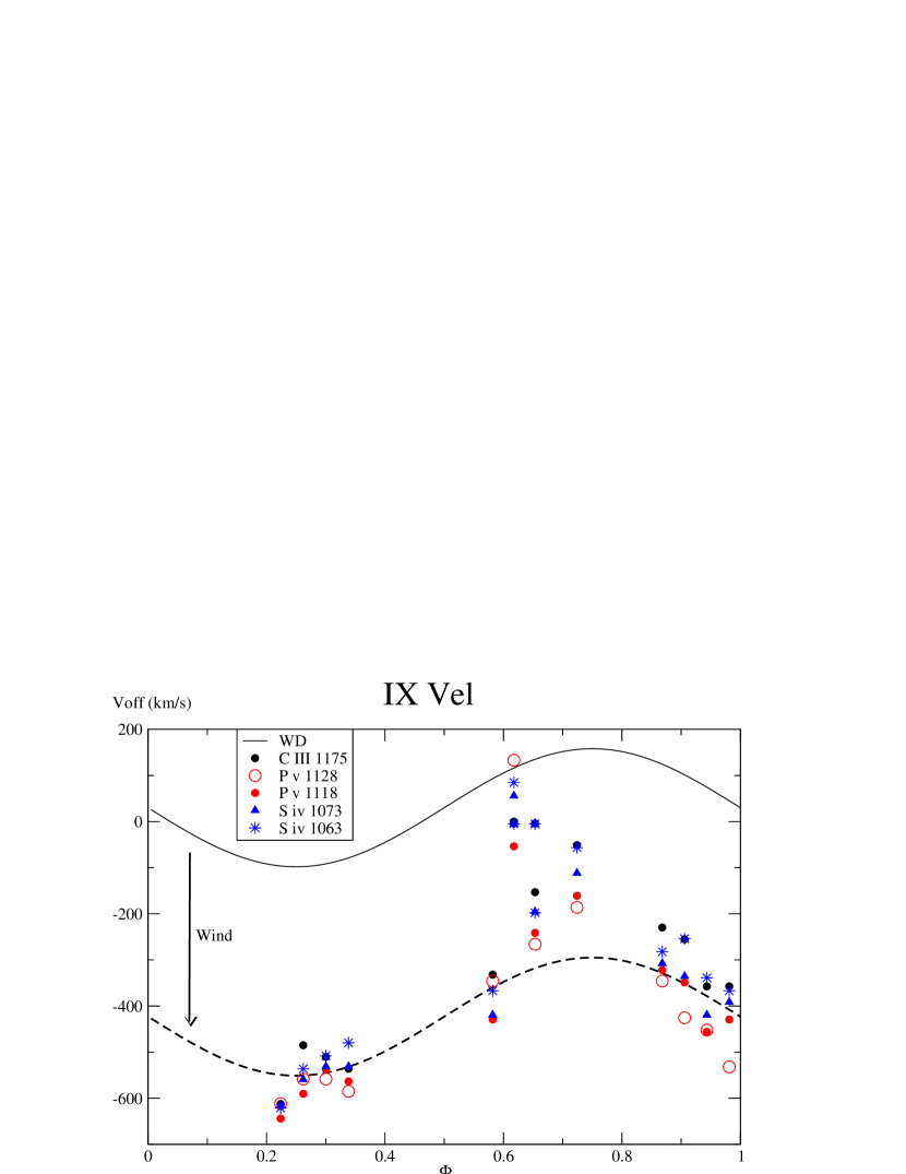
Figure 4: Velocity offsets (in km/s) of the most prominent absorption lines in the FUSE spectrum of IX Vel as a function of the orbital phase $\Phi$. IX Vel is always in state of high accretion rate where the disk dominates the FUV. The lines have been marked with symbols as indicated in the upper left. A WD velocity amplitude of 138km/s was taken from Beuermann & Thomas (1990) (solid black line). The lines are strongly blue shifted at most orbital phases. To account for the excess negative velocities, we assume a -450km/s wind velocity, and we move the WD radial velocity down by 450km/s (dashed black line). In such a configuration (dashed line) the overall pattern of the line velocity offsets as a function of the orbital phase is similar to that of U Gem (Fig.3d).

3 The Ballistic Trajectories

Our goal is to numerically follow the $L1$ stream as it leaves the $L1$ region, impacts the disk edge where it is deflected above the disk, and eventually lands onto the disk near phase 0.5-0.6. The radial velocity of the deflected stream in the line of sight of the observer is then to be compared to the radial velocity shift of the absorption lines in the FUSE spectrum of U Gem in outburst. In this section we present the numerical solver we have developed to carry out this task, under the assumption that the $L1$ stream can be represented by test particles following ballistic trajectories within the context of the Roche model in the restricted three-body problem. The specific description of the deflection of the stream by the disk edge is delayed to the next section.

To avoid any confusion, we stress here that in the manuscript we use the following notation (see also Figs.5, 6, & 7): $i$ is the inclination of the binary plane; $\Phi$ is the binary orbital phase; $\theta_{s}$ is the angle the $L1$ stream is making with the line joining the two masses as the stream leaves $L1$; $\varphi_{0}$ is the angle the $L1$ stream is making with the X-direction at the point it impacts the outer edge of the disk (before it is deflected); $\phi$ is the impact angle, it is measured counterclockwise from the line joining the two stars to the line joining the primary star to the site of impact of the stream on the disk; $\theta$ is the angle the bow shock makes with the horizontal (at any point $P$ on its surface), which under certain circumstances is equal to the launching angle at which the test particles are ejected off the shock front (the launching angle has a maximum $\theta_{\rm max}$); $\varpi_{\rm d}$ is the circularization radius, namely the radius at which the angular velocity of the test particle equals the Keplerian velocity; and $\varphi_{\rm h}-180^{\circ}$ is the circularization angle, the angle at which the stream impacts a disk of radius $R_{\rm disk}=R_{\rm d}=\varpi_{\rm d}$, measured counterclockwise from the line joining the two stars; in that case $\phi=\varphi_{\rm h}-180^{\circ}$ (Lubow & Shu, 1975).

3.1 Assumption and Equations

In the vicinity of the first Lagrangian point $L1$, the hydrostatic balance becomes less well satisfied as the stream flows, and the pressure force expands the stream width and thickness, increasing the stream scale height, until vertical forces drive the stream back toward the disk midplane. As the flow becomes hypersonic near the disk edge, the velocity field can then be regarded as nearly horizontal and the center of the gas stream can be described with test particles following ballistic trajectories in the restricted three-body problem (Lubow & Shu, 1975; Lubow, 1989, as long as the ballistic trajectories/orbits do not intersect).

The gaseous $L1$ stream is modeled by a finite number ($N=91$) of test particles moving under the influence of the gravitational potential of the binary masses. For each test particle, with coordinates $(x,y,z)$, we write the equations within the circular restricted three-body problem in the rotating (center of mass) frame of reference (Moulton, 1914; Plummer, 1918)

$$\left\{\begin{array}[]{l}\frac{dx^{2}}{dt^{2}}=+2\frac{dy}{dt}n+xn^{2}-Gm_{1}\frac{(x-x_{1})}{r_{1}^{3}}-Gm_{2}\frac{(x-x_{2})}{r_{2}^{3}},\\ \frac{dy^{2}}{dt^{2}}=-2\frac{dx}{dt}n+yn^{2}-Gm_{1}\frac{y}{r_{1}^{3}}-Gm_{2}\frac{y}{r_{2}^{3}},\\ \frac{dz^{2}}{dt^{2}}=-Gm_{1}\frac{z}{r_{1}^{3}}-Gm_{2}\frac{z}{r_{2}^{3}},\end{array}\right.$$ (1)

$${\rm where}~{}~{}~{}r_{1}=\sqrt{(x-x_{1})^{2}+y^{2}+z^{2}},~{}~{}~{}~{}~{}~{}~{}~{}r_{2}=\sqrt{(x-x_{2})^{2}+y^{2}+z^{2}},$$

where $G$ is the gravitational constant, $m_{1}$ is the mass of the WD (located at $(x_{1},0,0)$), $m_{2}$ is the mass of the secondary (located at $(x_{2},0,0)$), $n=\sqrt{G(m_{1}+m_{2})/a^{3}}$ and $a$ is the binary separation. We chose the units of length, mass and time such that (respectively) $a=1$, $m_{1}+m_{2}=1$ and $G=1$, which gives $n=1$. The equations simplify to

$$\left\{\begin{array}[]{l}\frac{dx^{2}}{dt^{2}}=+2\frac{dy}{dt}+x-(1-\mu)\frac{(x-x_{1})}{r_{1}^{3}}-\mu\frac{(x-x_{2})}{r_{2}^{3}},\\ \frac{dy^{2}}{dt^{2}}=-2\frac{dx}{dt}+y-(1-\mu)\frac{y}{r_{1}^{3}}-\mu\frac{y}{r_{2}^{3}},\\ \frac{dz^{2}}{dt^{2}}=-(1-\mu)\frac{z}{r_{1}^{3}}-\mu\frac{z}{r_{2}^{3}},\end{array}\right.$$ (2)

where we put $m_{1}=1-\mu$ and $m_{2}=\mu$ (with $\mu<1/2$).

3.2 The Second-order Runge-Kutta Method

The three second-order equations (2) are written as six first-order equations

$$\left\{\begin{array}[]{l}\frac{dv_{x}}{dt}=2v_{y}+\frac{\partial F}{\partial x},\\ \frac{dv_{y}}{dt}=-2v_{x}+\frac{\partial F}{\partial y},\\ \frac{dv_{x}}{dt}=\frac{\partial F}{\partial z},\end{array}\right.~{}~{}~{}~{}~{}~{}~{}~{}~{}~{}~{}~{}~{}~{}~{}~{}~{}~{}~{}~{}~{}\left\{\begin{array}[]{l}\frac{dx}{dt}=v_{x},\\ \frac{dy}{dt}=v_{y},\\ \frac{dz}{dt}=v_{z},\end{array}\right.$$ (3)

with

$$F=\frac{1}{2}\left(x^{2}+y^{2}\right)+\frac{1-\mu}{r_{1}}+\frac{\mu}{r_{2}}.$$

Or in a more compact notation, we have

$$\frac{df_{i}}{dt}={\cal{F}}_{i},~{}~{}~{}~{}~{}~{}~{}~{}(i=1,2,..6),$$

where ${\cal{F}}_{i}$ is a function of $f_{j}$’s $(j=1,2,..6)$.

We use a second-order Runge-Kutta method (“predictor-corrector”; e.g. Press et al. (1992)) to numerically integrate the particle trajectory and advance from $f_{i}^{0}$ to $f_{i}^{1}$ in a time $\Delta t$:

$$\left\{\begin{array}[]{l}f_{i}^{1/2}=f_{i}^{0}+{\cal{F}}_{i}^{0}\frac{\Delta t}{2},\\ f_{i}^{1}=f_{i}^{0}+{\cal{F}}_{i}^{1/2}\Delta t,\end{array}~{}~{}~{}~{}~{}~{}~{}(i=1,2,..6).\right.$$

The numerical integration of the equations to follow the ballistic trajectories of the test particles is begun in the vicinity of the first Lagrangian point $L1:(x_{0},y_{0},z_{0})$. This completes the description of our restricted three-body numerical solver.

3.3 The First Lagrangian Point - L1

The first Lagrangian point is an extremum of the Jacobi integral ($F$ + constant) located on the X-axis, and it is found by solving the quintic equation derived from the condition $\partial F/\partial x=0$. The quintic equation has the form

$$\rho^{5}-(3-\mu)\rho^{4}+(3-2\mu)\rho^{3}-\mu\rho^{2}+2\mu\rho-\mu=0,$$ (4)

where $\rho=x_{2}-x$, $x-x_{1}=1-\rho$, the first mass $1-\mu$ is located at $x_{1}$ and the second mass $\mu$ is located at $x_{2}$. The real positive root of this equation is given by (Moulton, 1914; Plummer, 1918)

$$\rho=\left(\frac{\mu}{3}\right)^{1/3}-\frac{1}{3}\left(\frac{\mu}{3}\right)^{2/3}-\frac{1}{9}\left(\frac{\mu}{3}\right)^{3/3}-\frac{23}{81}\left(\frac{\mu}{3}\right)^{4/3}+...$$ (5)

In the present work, we find the root of the equation by numerically increasing $\rho$ from 0 to 1, in steps of $10^{-6}$, namely, the $x$-coordinate of the first Lagrangian point, $x_{l1}$ is accurate to the sixth digit.

3.4 The Roche Lobe Radius

A convenient measure of the size of the Roche Lobe, and therefore of the maximum size of the accretion disk, is given by the radius $R_{L}$ of a sphere which has the same volume as the Roche lobe (Kopal, 1959). This radius can be approximated by the following expressions (Paczyński, 1971)

$$\left\{\begin{array}[]{lr}\frac{R_{L}}{a}=0.38+0.2\log{\frac{m_{1}}{m_{2}}},{}{}{}{}{}&0.523\leq\frac{m_{1}}{m_{2}}\leq 20,\\ \frac{R_{L}}{a}=0.46224\left(\frac{m_{1}}{m_{1}+m_{2}}\right)^{1/3},{}{}{}{}{}&0\leq\frac{m_{1}}{m_{2}}\leq 0.523.\end{array}\right.$$ (6)

3.5 Test Without and With a Disk

Since the $L1$ point is an equilibrium point, in order to integrate the ballistic trajectory of a particle, we need to place the particle at an infinitesimal distance $\epsilon>0$ from $L1$ and give it a small velocity $\eta>0$, otherwise the CPU time it takes for the particle to move is very long. This also ensures that the particle starts moving in the desired direction (i.e. in the Roche lobe of the primary star). We denote the coordinates of $L1$ by $(x_{L1},0,0)$, and place the particle on the X-axis at $x_{L1}+\epsilon$ with a velocity $v_{x}=\eta$. We first chose $\epsilon$ and $\eta$ large such that a test particle leaves the $L1$ region in a finite number of time steps (i.e. a few thousands). Next, we reduce the values $\epsilon$ and $\eta$ until we observe that the integrated trajectory remains constant, which gives $\epsilon=10^{-6}$ and $\eta=10^{-3}$. The time step is initially chosen to be very small, then it is increased until it is found to affect the accuracy of the integration. We find that $\Delta t=10^{-4}$ is large enough to carry out the integration in a reasonable CPU time, while it is small enough to give a good accuracy (as described below).

As an actual test of the ballistic trajectory solver, we chose to replicate some of the results obtained by Lubow & Shu (1975). We follow the ballistic trajectory of a test particle for different values of the binary mass ratio, first without a disk, and compute several parameters for comparison with the results of Lubow & Shu (1975). The first parameter is the angle $\theta_{s}$ that the gas stream is making with the X-axis as it leaves the $L1$ region. Since we are integrating the equations from $x_{L1}$, we measure $\theta_{s}$ by solving for $a$ and $b$ as

$$\theta_{s}=\lim_{x\rightarrow x_{L1}}(x-x_{L1})a+b.$$

The next parameter is the circularization radius $\varpi_{\rm d}$, i.e. the radius at which the angular velocity of the test particle equals the Keplerian velocity. We then place a disk of radius $R_{\rm disk}=\varpi_{\rm d}$, and measure the circularization angle $\varphi_{\rm h}-180^{\circ}$, the angle $\phi$ at which the $L1$ stream impacts the disk edge, measured counterclockwise from the line joining the two masses.

The values we obtained are listed in Table 2. We checked these values against those of Lubow & Shu (1975) and found them exact to within up to a few $10^{-4}$ of their relative values. This is about $0.01^{\circ}$ in the impact angle $\phi$, which is much smaller than the width of the phase angle $\Phi$ at which line velocity offsets are obtained, since the data is often binned to more than several 100s, corresponding to a few degrees ($\sim 1/100$ of the orbital periods).

Table 2: Test of the Ballistic Trajectories

Mass Ratio	$\theta_{s}^{(1)}$	$\theta_{s}^{(1)}$	$x_{L1}^{(2)}$	$\varpi_{\rm d}^{(3)}$	$\varphi_{\rm h}-180^{\circ(4)}$
$m_{2}/m_{1}$	a	b			(deg)
50.0000	38.8473	24.1549	-0.804949	0.403620	41.6369
30.0000	30.4367	23.4695	-0.762810	0.345029	46.2916
27.0000	28.8461	23.3210	-0.752768	0.333168	47.2562
25.0000	27.6724	23.2126	-0.745097	0.324583	47.9583
22.0000	26.0610	23.0201	-0.731694	0.310481	49.1218
20.0000	24.6615	22.8834	-0.721126	0.300119	49.9829
17.0000	22.4351	22.6447	-0.701887	0.282760	51.4453
16.0000	21.7397	22.5510	-0.694292	0.276412	51.9829
15.0000	21.0134	22.4509	-0.685943	0.269718	52.5555
12.5000	18.7703	22.1764	-0.660795	0.251257	54.1526
10.0000	16.3794	21.8330	-0.626603	0.229674	56.0519
8.50000	14.7875	21.5831	-0.599098	0.214695	57.4010
8.00000	14.2367	21.4900	-0.588236	0.209297	57.8883
7.00000	12.7447	21.2984	-0.563098	0.197727	58.9509
6.66667	12.2733	21.2272	-0.553484	0.193619	59.3329
5.50000	10.7305	20.9442	-0.513247	0.178097	60.7887
4.50000	8.94808	20.6732	-0.467151	0.163037	62.2355
4.00000	7.88968	20.5249	-0.438075	0.154758	63.0419
3.33333	6.53351	20.3029	-0.390097	0.142764	64.2243
3.00000	5.81271	20.1833	-0.360743	0.136275	64.8757
2.00000	2.90722	19.8145	-0.237418	0.114279	67.1305
1.66667	1.66566	19.6972	-0.177342	0.105850	68.0150
1.33333	0.14992	19.6010	-0.101000	0.096674	68.9854
1.29870	0.03820	19.5908	-0.091844	0.095658	69.1014
1.29032	-0.02100	19.5895	-0.089588	0.095428	69.1163
1.25000	-0.16319	19.5787	-0.078506	0.094236	69.2469
1.11111	-1.03684	19.5608	-0.037159	0.090024	69.6983
1.00000	-1.54800	19.5482	0.000000	0.086509	70.0732
0.750000	-3.28001	19.5878	0.101000	0.078010	70.9594
0.599988	-4.84861	19.6866	0.177349	0.072363	71.5456
0.500000	-6.17680	19.8050	0.237418	0.068302	71.9329
0.333333	-9.34664	20.1759	0.360743	0.060609	72.6460
0.300000	-10.1587	20.2907	0.390097	0.058871	72.7878
0.250000	-11.7016	20.5085	0.438075	0.056050	73.0183
0.222222	-12.8940	20.6642	0.467151	0.054348	73.1470
0.181818	-14.9364	20.9407	0.513247	0.051642	73.3225
0.150000	-16.7606	21.2100	0.553484	0.049224	73.4712
0.142857	-17.3286	21.2829	0.563098	0.048631	73.5107
0.125000	-19.0387	21.4884	0.588236	0.047066	73.5947
0.117647	-19.7009	21.5779	0.599098	0.046382	73.6193
0.100000	-21.6154	21.8218	0.626603	0.044584	73.7114
0.066667	-27.2200	22.4429	0.685943	0.040421	73.8607
0.062500	-28.1263	22.5387	0.694292	0.039794	73.8775
0.020000	-49.9464	24.1552	0.804949	0.029898	74.0799

(1) $\theta_{s}$ is the angle the $L1$ stream is making with the line joining the two masses as the stream leaves $L1$. To a first approximation $\theta_{s}\approx(x-x_{L1})a+b$. The value that has to be compared to Lubow & Shu (1975, Table 1) is $b$. (2) $x_{L1}$ the x-coordinate of the $L1$ point. (3) $\varpi_{\rm d}$ is the circularization radius, and (4) $\varphi_{\rm h}-180^{\circ}$ is the circularization angle (in Table 2 in Lubow & Shu, 1975).

4 Bow Shock Deflection

We now concentrate on the interaction of the incident $L1$ stream with the rim of the disk. While we consider only the region above the disk, namely for $z\geq 0$, a symmetrical picture holds below the disk for $z\leq 0$. As the stream leaves the $L1$ region, its interaction with the rim of the accretion disk can be summarized as follows:

(0) Because both the stream and disk are highly hypersonic, a bow shock develops at the impact region (Lubow & Shu, 1976; Armitage & Livio, 1998; Kunze et al., 2001).

(i) At an elevation $z$ high enough above the disk plane (i.e. for $z>H_{0}$, where $H_{0}$ is larger than the disk vertical scale height $H$), the $L1$ stream density becomes significantly larger than that of the disk, and stream material is able to pass above the disk without being affected by its presence (Lubow & Shu, 1975; Lubow, 1989).

(ii) Within the context of a hypersonic flow past a blunt object, we expect the stream matter to be deflected upward across the bow shock (Rathakrishnan, 2010). This is somewhat similar to the simulations of the isothermal case in Armitage & Livio (1998) and the $\gamma\approx 1$ polytropic case in Kunze et al. (2001).

(iii) At higher mass accretion rates, and/or if the $L1$ stream velocity is large, a heated region will develop in the shock, first in the vicinity of the disk midplane where the density is larger, then possibly in the entire shock region if cooling becomes inefficient. Here we consider the case in which the midplane region of the shock might be heated, but higher up, the shock is still behaving in a manner similar to the isothermal case.

(iv) Eventually, as cooling becomes inefficient, the entire shock region becomes hot enough to expand and stream matter might even be ejected due to adiabatic expansion. This is similar to the adiabatic case in Armitage & Livio (1998) and the larger polytropic coefficient simulations of Kunze et al. (2001) in which more stream matter is stopped at the hot spot region. One can expect here the hot spot to extend vertically and laterally and to even form a “tail”. In this case it is likely that a hot bulge forms (at the hot spot location) splashing in all directions without the formation of a coherent stream (Kunze et al., 2001).

In the present work, we concentrate only on the cases that can be approximated within the context of a nearly isothermal hypersonic flow past a blunt object forming a bow shock, namely cases (0), (i), (ii), and (iii). We do not consider additional scenarios such as for example a tilted disk, where the stream might completely miss the rim; or a thick disk impacted by a thin stream without overflow.

4.1 The Stream-Disk Interaction as a Hypersonic Flow past a Blunt Object

Since our main assumption rests on the hydrodynamical problem of the hypersonic flow past a blunt object, we consider now the general behavior of such a flow, with the $L1$ stream as the hypersonic flow and the disk as the blunt object. The general problem has been extensively studied analytically, numerically and in wind tunnel experiments, since it directly applies to the flight of a rocket/missile in the Earth’s atmosphere (e.g. Rathakrishnan, 2010).

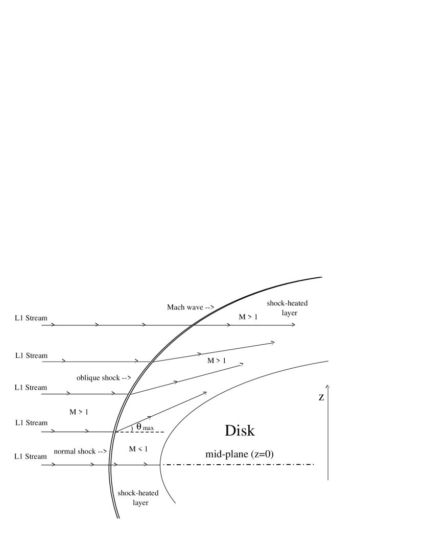
Figure 5: Schematic illustration of the $L1$ stream impacting the outer edge of the disk forming a bow shock. The hypersonic ($M>>1$) $L1$ stream flows in from the left and impacts the disk located on the right. For clarity, only the $z>0$ region is shown. At the stream-disk interface a bow shock forms, shown here with the double black line. By analogy with the hypersonic flow past a blunt body, one can differentiate between three regions. (1) Near the mid-plane of the disk (with a higher density) the shock is normal to the velocity and the downstream velocity is subsonic. (2) Higher up, the shock is oblique and the downstream velocity changes gradually from subsonic (strong shock) to supersonic (weaker shock) as $z$ increases. (3) At still higher elevation, as the shock weakens, it forms a Mach wave and the downstream velocity is hypersonic. The $L1$ stream material in region (3) continues mostly unaffected by the shock; at lower elevations, through the oblique shock in region (2) and the normal shock in region (1), the material is deflected upwards to a maximum angle $\theta_{\rm max}$.

We represent such a configuration with the disk seen edge-on in Fig.5. The $L1$ stream flows in from the left and impacts the disk located on the right. As a result a “detached” shock forms in front of the disk edge, in the shape of a bow: the bow shock. In the region near the disk midplane ($z\approx 0$), the shock is perpendicular (normal) to the velocity of the stream and the shock is the strongest there. Downstream from the normal shock, in the stagnation region (i.e. between the normal shock and the disk), the velocity is subsonic. As one moves away from the midplane along the bow shock (as $z$ increases), the shock becomes oblique and the downstream velocity changes gradually from subsonic (strong shock) to supersonic (weaker shock). Downstream from that region the flow is deflected upward. Farther away from the midplane, as the shock weakens, it forms a Mach wave (a weak shock) and the downstream velocity remains hypersonic. The $L1$ stream material high above the disk midplane, in the Mach wave region, continues mostly unaffected by the shock; at lower elevations, through the oblique shock and the normal shock, the material is deflected upward to a maximum angle $\theta_{\rm max}$. Across the bow shock, there is no change in the velocity component tangent to the shock; however, the velocity component normal to the shock is decelerated to a subsonic value.

4.2 Bow Shock Deflection off the Disk Plane

The vertical deflection of the the $L1$ stream by the bow shock can be formulated as follows. We simulate the trajectory of test particles from $L1$, assuming that the stream has a vertical extent ($z>0$) but flows horizontally ($V_{z}=0$) until it reaches the bow shock. At a given height, a test particle impacts the bow shock at a point ${\rm P}$, where the bow shock surface makes an angle $\theta$ with the plane of the disk (XY plane; see Fig.6, left panel). There, the component of the velocity normal to the shock surface is reduced to a subsonic value, while the component parallel to the shock remains unchanged. The particle velocity before impacting the disk $V=V_{x}^{2}+V_{y}^{2}$ is decomposed (Fig.6, right panel) into a component parallel to the direction of the deflection (making an angle $\theta$ with the $XY$-plane) $V_{\|}$ and a component perpendicular to the shock (making an angle $-(\pi/2-\theta)$ with the $XY$-plane) $V_{\bot}$.

We assume that before impact the velocity is hypersonic, such that $V={\cal{M}}c_{s}^{0}$, where $c_{s}^{0}$ is the sound speed before impact (upstream), and ${\cal{M}}>>1$. For example, Armitage & Livio (1998) assumed ${\cal{M}}=30$ in their isothermal case simulation, and we adopt here this value. After the shock, the perpendicular component $V_{\bot}$ of the velocity is set to subsonic; $V_{\bot}=\beta c_{s}^{1}$ with $0<\beta<1$ and $c_{s}^{1}$ is the sound speed after the shock (downstream). In the present case we chose $\beta=0.5$. Therefore, before impact one has:

$$\left\{\begin{array}[]{l}V_{\|}=V\cos{\theta},\\ V_{\bot}=V\sin{\theta},\\ V={\cal{M}}c_{s}^{0}.\end{array}\right.~{}~{}~{}~{}{\rm and}~{}~{}~{}~{}~{}~{}\left\{\begin{array}[]{l}V_{x}=V\cos{\varphi_{0}},\\ V_{y}=V\sin{\varphi_{0}},\\ V_{z}=0,\end{array}\right.$$ (7)

where $\varphi_{0}$ is the angle the velocity $\vec{V}$ is making with the X-axis (see Fig.7). After impact the velocity components become:

$$\left\{\begin{array}[]{l}V_{\|}={\cal{M}}c_{s}^{0}\cos{\theta},\\ V_{\bot}=\beta c_{s}^{1},\\ 0<\beta<1.\\ \end{array}\right.$$ (8)

Figure 6: Schematic model of the stream from the first Lagrangian point, $L1$, deflected across the bow shock. Left. The $L1$ stream material is moving from the left with a velocity $V$ and collides with the disk forming a bow shock. As a result, at any point $P$ matter is deflected across the bow shock and launched on a ballistic trajectory. The surface of the bow shock at $P$ forms an angle $\theta$ with the plane of the disk (horizontal). At the front of the shock, lower left, $\theta=90^{\circ}$, downstream to the right one has $\theta\rightarrow 0$. Right. The incoming (test) particle velocity components are decomposed.

We decompose $V_{\|}$ back into its $x,y,z$ components (Fig.6, right panel). Across the hot spot region, we therefore have

$$\left\{\begin{array}[]{l}V_{x}\rightarrow(c_{s}^{0}{\cal{M}}\cos^{2}{\theta}+c_{s}^{1}\beta\sin{\theta})\cos{\varphi_{0}},\\ V_{y}\rightarrow(c_{s}^{0}{\cal{M}}\cos^{2}{\theta}+c_{s}^{1}\beta\sin{\theta})\sin{\varphi_{0}},\\ V_{z}\rightarrow(c_{s}^{0}{\cal{M}}\sin{\theta}-c_{s}^{1}\beta)\cos{\theta}.\\ \end{array}\right.$$ (9)

If we now further assume that the shock is nearly isothermal, we have $c_{s}^{1}\approx c_{s}^{0}$ and

$$\frac{c_{s}^{1}\beta}{c_{s}^{0}\cal{M}}=\frac{0.5}{30}<<1.$$ (10)

We therefore drop the $c_{s}^{1}\beta$ term to simplify the expression (see also the discussion section). The velocities are reduced to:

$$\left\{\begin{array}[]{l}V_{\|}=V\cos{\theta},\\ V_{\bot}=V\sin{\theta}\rightarrow 0,\end{array}\right.$$ (11)

and decomposing $V_{\|}$ back into its $x,y,z$ components, we obtain

$$\left\{\begin{array}[]{l}V_{x}\rightarrow V_{x}\cos^{2}{\theta},\\ V_{y}\rightarrow V_{y}\cos^{2}{\theta},\\ V_{z}:~{}0\rightarrow\sqrt{V_{x}^{2}+V_{y}^{2}}\cos{\theta}\sin{\theta}.\\ \end{array}\right.$$ (12)

Under this assumption, the velocity perpendicular to the shock is simply set to zero, and the angle the shock is making with the XY plane, $\theta$, becomes the angle at which the particles are launched off the disk plane. Within the XY (disk) plane, the velocity of the particle keeps the same direction. For $\theta=0$, the particle velocity remains unchanged as it passes above the disk; for $\theta=\pi/2$, the particle velocity goes to zero as it impacts the disk mid-plane. Preliminiary results for this assumption only were presented for EM Cyg in Godon et al. (2009).

4.3 Second Assumption: Matching the Disk Keplerian Velocity

As the stream matter impacts the disk edge, in addition to being deflected off the disk plane, it is expected that the radial (directed from the WD) component of the stream velocity will be reduced or even possibly canceled, at least in these regions where the disk density is much larger than the stream density. At the disk midplane the radial component of the stream velocity must vanish, while at a few vertical disk scale heights $H$ the stream velocity (and direction) will not be affected at all.

Let us decompose the stream velocity $(V_{x},V_{y})$, before impact, in its tangential $V_{T}$ and radial $V_{R}$ components (see Fig.7),

$$\left\{\begin{array}[]{l}V_{R}=-V_{x}\cos{\phi}-V_{y}\sin{\phi},\\ V_{T}=V_{x}\sin{\phi}-V_{y}\cos{\phi},\end{array}\right.$$ (13)

where the angle $\phi$ defines the place where the stream hits the edge of the disk as viewed from the primary, in the disk plane, and it is measured counterclockwise from the line joining the two stars.

For stream matter impacting the disk edge at the midplane the radial component of the velocity vanishes completely, $V_{R}\rightarrow 0$, while for stream matter at several scale height $H$ above the disk $V_{R}$ remains unchanged, as the stream flow is not interacting with the disk. Similarly, we assume that the tangential velocity $V_{T}$ will match the Keplerian velocity $V_{K}$ at the disk edge for $\theta=\pi/2$ and will remain unchanged for $\theta=0$. We therefore introduce a function $\alpha$ of $\theta$, such that

$$\left\{\begin{array}[]{lcl}\alpha(\theta)\rightarrow 0&for&\theta\rightarrow\pi/2,\\ \alpha(\theta)\rightarrow 1&for&\theta\rightarrow 0,\\ 0<\alpha(\theta)<1&for&0<\theta<\pi/2.\end{array}\right.$$ (14)

With this definition, the velocity components are transforming as follows:

$$\left\{\begin{array}[]{l}V_{R}\rightarrow\alpha(\theta)V_{R},\\ V_{T}\rightarrow\alpha(\theta)V_{T}+[1-\alpha]V_{K},\end{array}\right.$$ (15)

Figure 7: Model of the $L1$ stream deflection in the XY plane. The $L1$ stream velocity, at the disk edge impact, makes an angle $\varphi_{0}$ with the X-axis. We adopt the notation $\phi$ for the angle at which the stream impacts the disk edge.

Choosing $\alpha(\theta)=\cos^{2}{\theta}$, from the previous subsection (equation 12, see also the Discussion section), gives:

$$\left\{\begin{array}[]{l}V_{R}^{\prime}=V_{R}\cos^{2}{\theta},\\ V_{T}^{\prime}=V_{T}\cos^{2}{\theta}+V_{K}\sin^{2}{\theta},\end{array}\right.$$ (16)

where the prime denotes the velocities after deflection. After the stream impacts the disk, the $(x,y,z)$ components of the velocity are given by the final expressions

$$\left\{\begin{array}[]{l}V_{x}^{\prime}=V_{x}\cos^{2}{\theta}+V_{K}\sin^{2}{\theta}\sin{\phi},\\ V_{y}^{\prime}=V_{y}\cos^{2}{\theta}-V_{K}\sin^{2}{\theta}\cos{\phi},\\ V_{z}=V\cos{\theta}\sin{\theta}.\end{array}\right.$$ (17)

For $\theta\rightarrow 0$ the particle trajectory is not deflected as it does not interact with the edge of the disk; rather it passes above the disk. For $\theta\rightarrow\pi/2$, the particles impact the mid-plane of the disk; it undergoes the largest change in its velocity, losing its inner radial (toward the WD) component and a gaining a Keplerian component in the tangential direction (e.g. motion in the disk around the WD; assuming that the outer radius of the disk is not too large; otherwise, the secondary gravitational potential has to be taken into account).

5 Simulations & Results

For each $L1$ stream particle (with index $i=0,1,..,90$) we simulate the impact with the disk by launching it on a ballistic trajectory from a point $P_{i}(R_{i},z_{i})$, where $z_{i}=H_{0}-\Delta z_{i}$, $\Delta z_{i}=H_{0}(i/90)$, and $R_{i}=R_{\rm disk}-\Delta z_{i}$, with a launching angle $\theta=i^{\circ}$ (see Fig.8). $H_{0}$ is the minimum height ($z$) at which the $L1$ stream flows unaffected by the disk - a measure of (half) the vertical thickness of the bow shock. $H_{0}$ is unknown; it is likely of the order of a few disk scale heights $H$. In the simulations, it is varied until the data fit the observations. Our choice of $\Delta z_{i}$ is consistent with the assumption that the $L1$ stream flow is not deflected if $z>H_{0}$. While the launching angle takes values from $0^{\circ}$ to $90^{\circ}$, the points $P_{i}$ are lined up on a curved diagonal, rather than an hyperbolic. We found that the exact shape (curved diagonal vs hyperbolic) of the curve has no noticeable effects on the results. Since $H_{0}/R\sim$ a few $H/R$, itself just a few percent, the effect of the curve defining $P_{i}$ is very small as long as the post-shock velocity is dictated by the angle of deflection. The velocity imparted to each particle is then given by equation (17) above with $\theta=0^{\circ}$ to $90^{\circ}$. The particle is then followed until it falls back onto the disk at $z\approx H$. In the limit $\theta\rightarrow 0$ and $\Delta z\neq 0$ we obtain the same result as Lubow (1989), namely that the particle falls back onto the disk around orbital phase 0.5-0.6 (see Fig.9). For $\theta\neq 0$ we obtain that the particle is launched and falls back onto the disk at an angle $\phi_{impact}>150^{\circ}$. As $\theta$ increases, the particle reaches a maximum height above the disk, while the impact point on the disk reaches a maximum angle of $\approx 180^{\circ}$ (see Figs.8 & 9).

Figure 8: Simulation of the bow shock deflection launching of the $L1$ stream material at the outer edge of the disk. On the left we show a nearly edge-on view, and on the right we show a top view. 7 ballistic trajectories, for test particles moving from left to right, are shown in black, the accretion disk edge is in red. The axis are in units of the binary separation centered on the primary WD star - the red circle (not to scale) located at $(0,0)$. Trajectory a represents a particle passing at a height $z=H_{0}$ above the disk, which is not deflected at all, corresponding to a launching angle $\theta=0$. Trajectory g represents a particle hitting the disk at $z=0$ and being dragged with the Keplerian flow, corresponding to a launching angle $\theta=90^{\circ}$. For clarity we show only 7 partial trajectories, with launching angles as follows: $\theta=0^{\circ}$ (a), $\theta=15^{\circ}$ (b), $\theta=30^{\circ}$ (c), $\theta=45^{\circ}$ (d), $\theta=60^{\circ}$ (e), $\theta=75^{\circ}$ (f), and $\theta=90^{\circ}$ (g). The trajectories do not intersect. In the configuration shown the mass ratio is $m_{2}/m_{1}=0.35$, the disk outer radius $R_{\rm disk}=0.376a$ ($a$ is the binary separation), and $H_{0}/R=0.10$.

Figure 9: Three-dimensional perspective view of the binary at an inclination angle of $70^{\circ}$ and orbital phase $\Phi=0$ (the secondary is in front). The configuration is the same as in Figs.8, except that 19 particles are shown with deflection angles $\theta=0^{\circ}$, $5^{\circ}$, $10^{\circ}$,$15^{\circ}$, …, $85^{\circ}$, and $90^{\circ}$.

5.1 U Gem Input System Parameters

We now model the velocity offsets as a function of the orbital phase for the centers of the absorption lines in the FUSE spectrum of U Gem taken during an outburst (Froning et al., 2001). For that purpose, we review and discuss U Gem system parameters, as they are used as input parameters in the simulations.

Orbital Period and Masses.

U Gem has a period of 0.1769061911 days (4.24574858 hr; (Marsh et al., 1990; Echevarría et al., 2007; Dai & Qian, 2009)), and a mass ratio $q=0.35-0.362$ (Long & Gilliland, 1999; Smak, 2001; Echevarría et al., 2007). In the following, we scale the velocity offsets to the WD maximum radial velocity (amplitude) both in the observations and in our simulations. As a consequence, the WD mass per se does not explicitly enter into our simulation; it enters implicitly in the mass ratio. This has the advantage of being independent of the WD mass, as its value could be anywhere between $1.05M_{\odot}$ (Naylor et al., 2005; Echevarría et al., 2007, as inferred from scaling the UV flux to the known distance) and $1.25M_{\odot}$ (Sion et al., 1998; Long & Gilliland, 1999; Naylor et al., 2005; Echevarría et al., 2007, derived from the gravitational redshift). In the simulations we set $q=0.35$.

Inclination and Eclipsing Geometry.

U Gem is a partially eclipsing binary (Krzeminski, 1965), as the disk undergoes partial eclipses (at phases 0.95-0.05; Echevarría, de la Fuente, & Costero (2007)), the hot spot undergoes full eclipses, while the WD itself is not eclipsed at all (Smak, 1971; Warner & Nather, 1971). This restricts the inclination to be in the range $67^{\circ}$${}^{+7^{\circ}}_{-5^{\circ}}$ (Long & Gilliland, 1999; Long et al., 2006), though Long & Gilliland (1999) adopted $67^{\circ}\pm 3^{\circ}$. A value $i=69.7^{\circ}\pm 0.7^{\circ}$ was first derived by (Zhang & Robinson, 1987), which has been reassessed since then. A low inclination ($\sim 65^{\circ}$) is consistent with a large WD mass ($\sim 1.25M_{\odot}$), while a larger inclination ($\sim 73^{\circ}$, Unda-Sanzana et al. (2006)) is consistent with a smaller WD mass ($\sim 1.05M_{\odot}$). The larger WD mass has been corroborated by its gravitational redshift measurement, but the corresponding smaller WD radius is inconsistent with the UV flux scaling to the distance of the system. For that reason, we consider inclinations from $i=62^{\circ}$ to $i=75^{\circ}$.

The Outer Radius of the Disk.

The outer radius of the disk is expected to be larger during outburst than during quiescence (Smak, 2001) such that eclipses of the hot spot are not always observed (Marsh et al., 1990), and the secondary undergoes partial eclipses by the disk of only a few percent (Smak, 1971). The hot spot eclipses undergo a phase shift and occur earlier as the brightness rises; when the systems fades, the eclipses return to the original phase (Krzeminski, 1965). Since these are the eclipses of the hot spot by the secondary, this implies that the hot spot moves on the rim of the disk toward the secondary (retrograde motion) during the rise to outburst and vice versa during decline. For this to happen, the disk outer radius has to grow during rise and it has to decrease during decline, and one then expects the radius of the disk during quiescence to be rather small. However, Echevarría et al. (2007) report a symmetric full disk with an outer disk radius in deep quiescence of $0.61$ the binary separation, or about twice as large as expected (e.g. Lubow (1989)). Such a large disk radius almost reaches the first Lagrangian point $L_{1}$ and is larger than the average Roche lobe radius itself. The largest quiescent disk radius obtained by Smak (2001) was $\sim 0.5$ the binary separation, namely, 20% smaller. It is likely that not all outburst cycles show the same behavior, and consequently the outer radius of the accretion disk has to be considered as an unknown parameter. In the simulations, we vary the outer radius of the disk from $\sim$0.20 a to $\sim$0.60 a.

The Bow Shock Height $H_{0}$.

The minimum height $H_{0}$, at which the stream flows unaffected by the disk, corresponds in our model to a measure of the vertical thickness of the bow shock. $H_{0}$ is possibly of the order of a few disk scale heights $H$ and is taken as an additional unknown parameter. We vary $H_{0}/r$ from 0.02 to 0.30.

5.2 Output: Particle Coordinates and Velocities

Our restricted three-body code solves the particles coordinates and velocities as a function of time. The coordinates as a function of time provide the trajectories of the particles in three dimensions. We carry out a transformation of the trajectories (paths) of the particles into an inertial frame of reference as the three-dimensional projection viewed by the observer for a given orbital inclination $i$ and orbital phase $\Phi$. An example is given in Fig.10, where, for convenience, the graph and its axis in each panel are centered on the WD.

Figure 10: Perspective view of the binary configuration with the $L1$ stream launched above the disk at phase $\Phi=0.5$ (upper left), 0.6 (upper right and so on), 0.7, 0.8, 0.9, and 1.0. The secondary is in blue, the stream is in black and the accretion disk outer edge is represented with the large red circle. The smaller inner red circle delimits the inner region of the disk that is being veiled by the stream: the radial velocities of the stream test particles are only being considered inside this region (see text). Only 10 ballistic trajectories are being considered in this figure, with launching angles $\theta=0^{\circ}$, $5^{\circ}$, $10^{\circ}$,..,$40^{\circ}$, $45^{\circ}$. In the simulation shown in the figure, the veiling of the inner disk by the stream material begins a little before phase $\Phi=0.6$ (the ingress), and ends around phase $\Phi\approx 0.9$ (the egress).

The FUSE spectrum of U Gem, taken while the disk dominated the FUV, has a wavelength range of $\sim 910-1185$ Å. This implies that the inner accretion disk (the hottest region of the disk) is the predominant region contributing to the FUSE spectrum, while the outer disk emits in the optical, and the intermediate region emits mainly in the near-UV. As a consequence, it is the veiling of the inner disk by the $L1$ stream material that is responsible for the velocity offsets of the metal absorption lines as measured in the FUSE spectrum. We delimit the inner disk region with a radius $R_{v}$ (the veiling radius), and we only consider particles veiling the disk in the region $R<R_{v}$ (for a given inclination and as a function of the orbital phase, see Fig.10). The size of the veiling radius $R_{v}$ is a variable to be found.

Each point on a trajectory has a corresponding velocity, and we therefore consider the velocity of these partial trajectories within $R<R_{v}$. For each individual particle (each with a different launching angle $\theta$), we average the projected (to the observer) radial velocity over the partial trajectory delimited within $R<R_{v}$. Doing so, we obtain for each particle (i.e. for each angle $\theta$) an average radial velocity as a function of the orbital phase $\phi$ (for a given inclination).

In addition, we have to consider the fact that at some specific phases, such as e.g. 0.6 and 0.9 in Fig.10, the stream veils only a fraction of the inner disk. These are transition regions, similar to eclipse ingress and egress, and we do not expect the stream material to generate noticeable absorption lines if it covers less than 50% of the inner disk.

5.3 Results

We ran many simulations varying the parameters as described in the previous section, and we present the results by drawing the particle average radial velocity (see previous subsection) as a function of the orbital phase for direct comparison with the velocity offsets of metal lines of U Gem. For that purpose, Froning et al’s data have been slightly improved. Namely, the WD velocity has been adjusted to match the slightly larger amplitude as derived in Long et al. (2006). We also used the latest value of the ephemeris (Echevarría et al., 2007) and included heliocentric corrections that increase the orbital phases of the all the observed data points by $\sim 0.05$. The velocities have all been normalized to the maximum projected orbital velocity of the WD ($=1$).

For each simulation, the model is drawn on top of the observation as shown in Fig.11. We carry this procedure while changing the orbital inclination $i$, the outer radius of the disk $R_{d}$, and the thickness $H_{0}/r$. For each such simulation ($i$, $R_{d}$, $H_{0}/r$), we check the results for a range of launching angles $\theta$ (i.e. for a number of particles) and veiling radius $R_{v}$. In this procedure we try to match the velocity offset peak ($V_{\rm off}=5.2)$, the orbital phase of the peak $\Phi\approx 0.72-0.77$, and the velocity offset drop observed at phase $\Phi=0.81-0.82$. In Fig.11 we show two models with $i=66^{\circ}$ and $i=70^{\circ}$ to illustrate our technique. The model with the higher inclination produces a velocity maximum in excess of 6, and in both models the velocity peaks a little after phase $\Phi=0.8$. The phase at which the velocity offset peaks depends strongly on the outer radius of the disk, and the maximum velocity decreases with decreasing inclination and decreasing thickness $H_{0}$.

Consequently, we are able to better match the data by decreasing the disk radius while keeping the orbital inclination at $i=66^{\circ}$. We present this model in Fig.12. In this model $H_{0}/r=0.08$, and the maximum launching angle we obtained is $\theta=43^{\circ}$. The need to keep $\theta\leq 43^{\circ}$ is due to the minimum velocity ($\sim 3.69$) observed at phase $\Phi=0.72-0.77$: for $\theta>43^{\circ}$ the model produces lower velocity at that phase. The veiling radius is $R_{v}=0.025a$, it also dictates the lowest velocity, and especially around phase 0.8 at which the velocity drop is observed. A significantly larger veiling radius is ruled out because it would include particles with lower velocities, adding theoretical data points to the model with radial velocity of $\sim 3$ at phase $0.7-0.8$ (as seen in Fig.11 for $i=66^{\circ}$), which is not seen in the observational data.

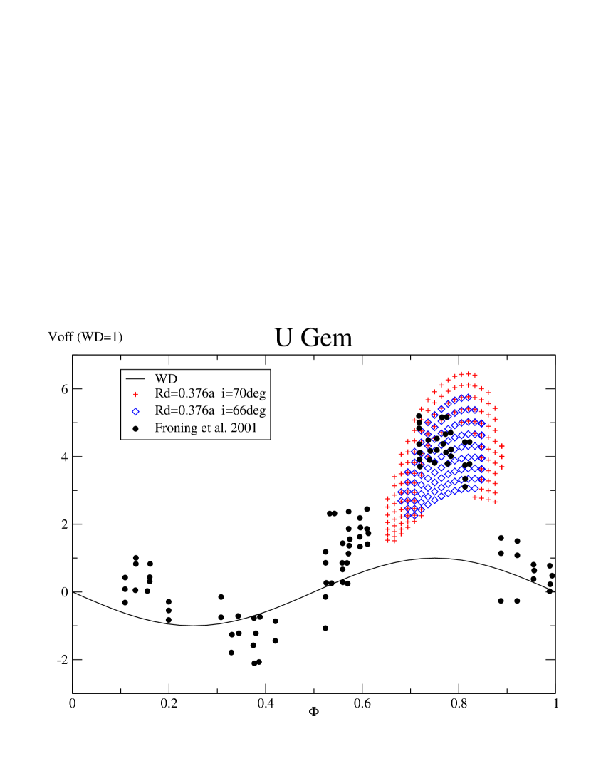
Figure 11: Velocity offsets of metal absorption lines in the FUSE spectra of U Gem obtained in outburst as a function of the orbital phase (from Froning et al. (2001), as in Fig.3d, all the circles are now filled), together with two ballistic trajectory models. Two stream-disk overflow ballistic trajectory simulations are shown for comparison assuming a relatively large outer radius for the disk, $R_{d}=0.376a$, $H_{0}/r=0.10$, and a binary inclination of $i=70^{\circ}$ (red crosses) and $i=66^{\circ}$ (blue diamonds). The lower inclination agrees better with the a maximum velocity of $\sim 5-6$, but both models are off-phase by $\sim 0.05-0.10$. Note that between phase $\sim 0.6-0.7$ there are no data points for comparison.

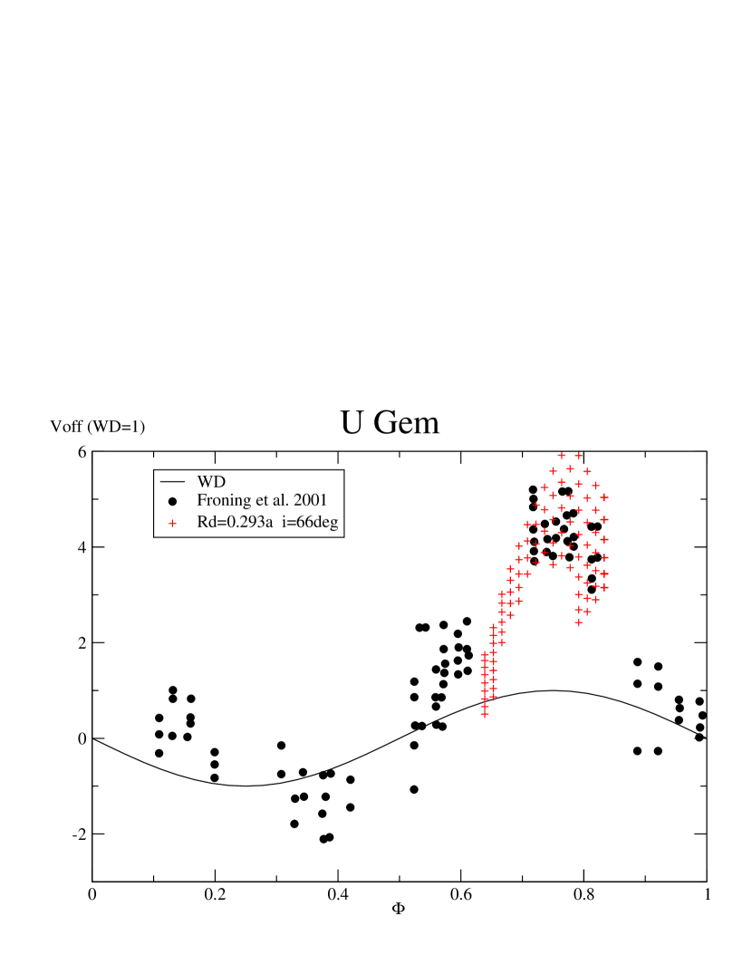
Figure 12: Velocity offsets of metal absorption lines (filled black circles) of U Gem in outburst as a function of the orbital phase as in the previous figure, together with a ballistic trajectory model (red crosses). Matching the observed data is obtained by decreasing the inclination of the model to $i=66\pm 1^{\circ}$ and setting the outer disk radius to $R_{d}=0.29\pm 0.023a$. The model is able to reproduce the drop in velocity seen around phase $\sim 0.8$. In this model $H_{0}/r=0.08\pm 0.02$ and the portion of the inner disk that is masked by the stream is within $r\leq 0.025\pm 0.005a$. At the edge of the disk the test particles are launched at a deflection angle of up to $43^{\circ}$.

6 Discussion

Overall, our results are able to reproduce the velocity shift of the absorption lines and are consistent with some of the system parameters (i.e. inclination, mass ratio,etc..). However, some of the approximations and assumptions we made are crude (e.g., isothermal) while other parameters (e.g. thickness $H_{0}$, outer radius) are actually unknown. We therefore need to address the values of the parameters we chose and how they affect the results, and check whether our assumptions are self-consistent.

Bow Shock Thickness $H_{0}$.

We obtained a bow shock (half) vertical thickness of $H_{0}/r=0.08\pm 0.02$, which was found by fitting the maximum velocity offset and its phase. Since $H_{0}$ is of the order of a few $H$, this result is consistent with the thin-disk approximation (Pringle, 1981) in the standard disk theory. If we consider a Keplerian disk with a midplane temperature of 12,000 K at the shock location (as expected for the “hot” spot), we obtain $H/r=c_{s}/V_{K}=0.02$, and $H_{0}/H=4$. For comparison, Lubow (1989) chose $H\sim 0.01a$, where $a$ is the binary separation, which for a disk of diameter $R_{\rm disk}=0.3a$, gives $H/r\approx 0.03$ at the edge disk; in that case $H_{0}/H=2.67$. The disk thickness $H$ does not enter the simulations anywhere, except for the constrain $H_{0}>H$. The particles are deflected there from an initial height $z_{i}=(1-i/90)\times H_{0}$. Hence, the thickness $H_{0}$ only gives an estimate of the initial height from where the $L1$ stream is deflected. It is also possible that the impact of the stream on the rim of the disk causes the disk to thicken there, due, for example, to shock heating near the midplane of the disk. In that case our isothermal assumption might still hold away from the mid-disk plane, which is from where the particles are launched.

Outer Disk Radius.

From our modeling, the actual location of the outer disk radius is within about $H_{0}$ from $R_{\rm disk}$, since this defines the region from where the stream material is launched. We therefore choose $H_{0}/2$ as the error in the radius of the disk. Since $H_{0}/r=0.08$, we take $0.04\times 0.29a\approx 0.012a$ as a first error. An additional error of $0.05R_{L}=0.021a$ is introduced as the step by which the outer disk radius was increased from simulation to simulation. As a consequence, the outer disk radius we obtained is $0.29a\pm 0.023a$, which is smaller than the tidal cutoff radius ($0.33a$; e.g. Linnell et al. (2009)). For a larger disk outer radius, the stream has less velocity, it veils the inner disk and impacts the disk at a later phase, and vice versa (see also Kunze et al., 2001). The outer radius was obtained by fitting the phase of maximum velocity offset, and it agrees with the theoretical expectation.

Inclination.

We obtained an inclination of $66^{\circ}\pm 1^{\circ}$, which is consistent with the value derived by Long & Gilliland (1999); Long et al. (2006) ($67^{\circ}\pm 3^{\circ}$) but noticeably lower than that in Unda-Sanzana et al. (2006) ($72^{\circ}$). The (relatively) lower inclination we found is needed to decrease the velocity maximum and its phase. The simulations were run in incremental steps of $1^{\circ}$ in $i$ and we therefore take the error to be $1^{\circ}$.

Launching Angle $\theta$ & Further Hydrodynamical Considerations.

Each simulation includes 91 particles, with launching angle $\theta=0^{\circ},1^{\circ},2^{\circ},..,89^{\circ},90^{\circ}$. And for each simulation we selected the particles agreeing with the data. The model that agreed best with the U Gem data included particles with $\theta<44^{\circ}$, i.e. $43^{\circ}$ was the maximum launching angle. While it may seem that adjusting $\theta$ in the model is an empirical fit, deflection of hypersonic flow past a blunt object is actually limited to a maximum angle $\theta_{\rm max}$ (see subsection 4.1). The fact that we obtained a maximum deflection angle is therefore consistent with the basic hydrodynamical assumption. Including particles with a deflection angle $\theta>43^{\circ}$ causes the model to depart from the data. Furthermore, particles that have larger deflection angle (say, as $\theta\rightarrow 90^{\circ}$) represent the stream material hitting the disk near its denser midplane region, where the material strong interaction with the disk prevents it from being launched (i.e. the deflection/launching assumption is not valid anymore, as pressure effects due to heating may take place, the vertical velocity decreases to zero, and the material is being dragged into a Keplerian orbit with the disk material).

Veiled Inner Region.

By fitting the data, we obtained a veiling region with a radius $R_{v}=0.025a$, which translates into $\sim 1/12$ of the outer radius of the disk or 8 times the WD radius ($8R_{\rm wd}$). For a $\sim 1M_{\odot}$ WD accreting at a mass accretion of near $10^{-8}M_{\odot}$/yr (Froning et al., 2001), the veiled inner disk, with $R<8R_{\rm wd}$, has a temperature of $T\sim 30,000$ K and larger (the standard disk model, e.g. Pringle (1981)). This is consistent with that region being the main FUV component in the FUSE spectral range. The outer disk with $T<20,000$ K ($r>16R_{\rm wd}$) does not contribute much flux in the FUSE range. And the disk region with $T\approx 25,000\pm 5,000$ K (contained within $16>r/R_{\rm wd}>8$) contributes less than 1/5 of the hotter inner region ($r/R_{\rm wd}<8$). The size of the veiled region we obtained is therefore consistent with being the main disk region contributing to the FUSE spectrum.

The $c_{s}^{1}\beta$ Term.

In section 4.2, we set the component $c_{s}^{1}\beta$ of the downstream velocity perpendicular to the shock surface to zero , by assuming that in the isothermal case it is negligible (equation 10). We ran simulations taking that term into consideration (equation 9), and obtained a difference of $1^{\circ}$ in the launching angle $\theta$, which produces the same results within the error bars.

The Choice of the Function $\alpha(\theta)$.

We also checked different functions $\alpha(\theta)$ (equations 14 & 15) and found that the exact form of the function had no noticeable effect on the results.

Isothermal Assumption.

The assumption of an isothermal flow is explicitly made in equation 10 (i.e. assuming $c_{s}^{1}=c_{s}^{0}$), but it is also implicitly made in our most basis assumption that the stream-disk interaction can be represented as a hypersonic flow past a blunt body. In the flow past a blunt body we assumed that the stream is deflected due to the presence of the shock (or ‘solid’ disk surface), rather than due to the adiabatic expansion of the heated gas. We expect this assumption to break down near the disk midplane where the shock is the strongest and heating is likely to occur. However, that portion of the flow does not contribute to the computational data since the launching angle occurs for the upper portion of our simulated bow shock with $\theta<44^{\circ}$. This validates the isothermal assumption as self-consistent.

Stream Density and Depth of the Absorption Lines.

The ballistic trajectories (particle paths) define a strip (i.e. a 2D surface like a curtain) that masks the inner disk, and the (projected) density of the trajectory “lines” is a likely indicator of the relative projected thickness of the stream. However, as we do not take the pressure effects into account, the vertical and lateral expansion of the stream, that is likely decreasing its density and turning the strip into a three-dimensional conduit, is ignored. Our simulations also do not include any assumption about the actual mass accretion rate. In other words, we did not make any theoretical attempt to derive the stream density, and, as a consequence, we cannot predict whether the stream has the adequate density to produce the depth of the observed absorption lines. Instead, we assume a priori that the absorption lines could be forming in the stream and we check our assumption a posteriori by fitting the velocity offsets of the absorption lines with the projected radial stream velocity.

Full Phase Dependence Absorption.

The data reveal absorption lines increasing in depth and the sudden appearance of low-ionization lines at orbital phase $\sim 0.70\pm 0.15$ (Froning et al., 2001; Long et al., 2006; Godon et al., 2017), which are the same orbital phases as the X-ray and EUV light-curve dips seen in U Gem in both outburst and quiescence (Mason et al., 1988; Long et al., 1996; Szkody et al., 1996). Our ballistic trajectory modeling clearly shows how the $L1$ stream can veil the inner disk and WD and explains the change in the absorption lines as a function of the orbital phase, where the exact veiling phase depends on the size of the disk. The increase in the depth of the absorption lines, however, has also been observed around orbital phase 0.2-0.35 (Long et al., 2006; Godon et al., 2017), and Kunze et al. (2001) had shown, using smoothed particle hydrodynamics simulations, that parts of the overflowing stream can bounce off the disk face after hitting it at orbital phase 0.5, creating an additional absorption region observed around orbital phase 0.2-0.35 (Froning et al., 2001; Long et al., 2006; Godon et al., 2017). We therefore decided to run the simulations further by allowing the particles to bounce off the disk face. The reflected particles then continue on a trajectory reaching a maximum altitude (z) and distance (R) from the WD around phase 0.20-0.25 (see Fig.13 upper left), and then fall back toward the disk (Fig.13 upper right). There the particles continue on a trajectory that either intersects the disk a second time or moves below to the other side of the disk. We stopped the simulations before this happens. We then draw, in Fig.13 lower panel, the projected radial velocity of the particles veiling the inner disk as a function of the phase for comparison with the observed velocity offsets of the metal absorption lines. The reflected ballistic trajectory model is able to reproduce the phase (0.2-0.35) at which the secondary absorption lines are observed. In addition, the particle radial velocity agrees with the velocity offsets where there are actual data. In the regions where the stream only partially veils the inner disk (in blue in Fig.13, lower panel), we do not expect the absorption-line velocity to be significantly affected by the stream. This is especially the case around phase 0.6. The reflected stream spreads more than the incident stream and one might therefore expect that the veiling curtain is thinner around phase 0.2-0.35 than around phase 0.7-0.8.

Figure 13: The deflected incident $L1$ stream is allowed to bounce back off the disk face (near phase 0.5). The simulation is stopped as the stream continues toward phase 0.1, before it either bounces back off the disk a second time or reaches the other face of the disk. The top two panels show the ballistic trajectories in the physical space: face-on (left) and in perspective at phase 0.0 (right). The lower panel show the resulting projected (toward the observer) radial velocity as a function of the phase (as in Figs.11 & 12). We have now added the theoretical data points for the bouncing stream (green crosses). The stream covering less than $\sim 50$% of the inner disk (at ingress and egress) has been marked with blue squares.

7 Summary & Conclusion

Within the context of the Roche model in the restricted three-body problem, we model the interaction of the $L1$ stream with the accretion disk using ballistic trajectories, assuming that the stream-disk interaction can be represented as a hypersonic flow past a blunt object. Assuming that pressure effects are negligible and that the flow is isothermal, the bow shock deflects the stream material and launches it into ballistic trajectories. The $L1$ stream material veils the inner disk and is suspected to be responsible for affecting absorption lines in spectra of high inclination interacting binaries around orbital phase $\sim 0.75$. Using this formalism, we model the velocity offsets of metal absorption lines of U Gem in outburst at orbital phase $\sim 0.70-0.85$. The simulations match the velocity and phase of the lines for the following system parameters: a mass ratio $q=m_{2}/m_{1}=0.35$, an inclination $i=66\pm 1^{\circ}$, an outer disk radius $R_{\rm disk}=0.29a\pm 0.023a$, a measure of the bow shock vertical thickness $H_{0}/r=0.08\pm 0.02$, and the portion of the inner disk that is veiled by the stream is confined to $r\leq R_{v}=0.025a\pm 0.005a$, where $R_{v}$ is the radius of the inner disk that is veiled by the stream and $a$ is the binary separation.

In our ballistic streamline approximation we neglected pressure effects, and as a consequence, we did not address the width and thickness of the stream, nor its vertical density structure and scale height. Therefore, our model cannot predict whether the stream has the adequate density to produce the depth of the observed absorption lines.

Because of all the simplifications and assumptions in our model, it is likely that the actual values of the outer disk radius, the thickness of the bow shock, and the size of the veiled inner disk are in fact different than derived here. It is also very likely that, during U Gem outburst, $\dot{M}$, $R_{\rm disk}$, $H_{0}$ and $R_{v}$, all vary with time. In spite of these, our results provide increased evidence for the stream overflow model to explain the velocity offsets of the absorption lines.

Stream-disk overflow is possibly a prominent and important feature in most systems with Roche lobe overflow with a disk, as a substantial part of the accretion stream can overflow the disk in many different systems, in some cases with matter settling around the circularization radius (Kunze et al., 2001). Observations of semi-detached interacting binaries indeed reveal orbital modulation in the optical, ultraviolet, and X-ray bands consistent with the presence of $L1$ stream material overflowing the disk edge.

We suggest ballistic trajectories as a computational tool for the analysis of the absorption-line orbital variability in semi-detached binaries. This method could also be used with the limitations mentioned above, to assess or confirm the system parameters such as the mass ratio, inclination, and disk outer radius. This formalism can be applied to systems under certain restrictions, namely, when the launching of the material is occurring in a shocked region of the stream-disk interaction that is isothermal and where pressure and adiabatic effects can be neglected.

References

- Agafonov et al. (2009) Agafonov, M., Sharova, O., & Richards, M., 2009, ApJ, 690, 1730
- Armitage & Livio (1996) Armitage, P.J., & Livio, M. 1996, ApJ, 470, 1024
- Armitage & Livio (1998) Armitage, P.J., & Livio, M. 1998, ApJ, 493, 898
- Beuermann & Thomas (1990) Beuermann, K., & Thomas, H.-C. 1990, A&A, 230, 326
- Billington et al. (1996) Billington, I., Marsh, R.T., Horne, K., Cheng, F.H., Thomas, G., Bruch, A., O’Donoghue, D., & Eracleous, M. 1996, MNRAS, 279, 1274
- Bisikalo et al. (2000) Bisikalo, D.V., Boyarchuk, A.A., Kuznetsov, O.A., & Chechetkin, V.M. 2000, Astron.Report, 44, 26 (from Russian: Astro.Zhurnal 77, 2000, 31)
- Bisikalo et al. (2003) Bisikalo, D.V., Boyarchuk, A.A., Kaygorodov, P.V., & Kuznetsov, O.A., 2003, Astron.Rep., 47, 809 (from Russian: Astro.Zhurnal 80, 2003, 879)
- Bisikalo et al. (2005) Bisikalo, D.V., Kaygorodov, P.V., Boyarchuk, A.A., & Kuznetsov, O.A. 2005, Astron.Rep.49, 701 (originally in Russian: Astron.Zhurnal vol. 82, N.9, 2005, pp. 788-796)
- Blondin (1998) Blondin, J.M. 1998, API Conf.Proc. 431, 309
- Csizmadia et al. (2008) Csizmadia, Sz., Nagy, Zs., Borkovits, T., Hegedüs, T., Biro, I.B., & Kiss, Z.T. 2008, AN 329, 39
- Dai & Qian (2009) Dai, Z., & Qian, S. 2009, ApSS, 321, 91
- Dhillon et al. (1997) Dhillon, V.S., Marsh, T.R., & Jones, D.P.H. 1997, MNRAS, 291, 694
- Echevarría et al. (2007) Ecchevarría, J., de la Fuente, E., & Costero, R. 2007, ApJ, 134, 262
- Frank et al. (1987) Frank, J., King, A.R., & Lasota, J.P. 1987, A&A, 178, 137
- Froning et al. (2001) Froning, C.S., Long, K.S., Drew, J.E., Knigge, C., & Progra, D. 2001, ApJ, 562, 963
- Godon et al. (2017) Godon, P., Shara, M.M., Sion, E.M., & Zurek, D. 2017, ApJ, 850, 146
- Godon et al. (2009) Godon, P., Sion, E.M., Barrett, P.E., & Linnell, A.P. 2009, ApJ, 699, 1229
- Godon et al. (2006) Godon, P., Sion, E.M., Cheng, F., Long, K.S., Gänsicke, B.T., et al. 2006, ApJ, 642, 1018
- Hack & La Dous (1993) Hack, M., & La Dous, C. 1993, Cataclysmic Variables & Related Objects, (NASA SP-507)/US Gov.Printing Office
- Harrison et al. (2004) Harrison, T.E., Johnson, J.J., MaArthur, B.E., Benedict, G.F., Szkody, P., Howell, S.B., & Gelino, D.M. 2004, AJ, 127, 460
- Hartley et al. (2002) Hartley, L.E., Drew, J.E., Long, K.S., Knigge, C., & Proga, D. 2002, MNRAS, 332, 127
- Hellier (1996) Hellier, C. 1996, ApJ, 471, 949
- Hellier & Robbinson (1994) Hellier, C., & Robbinson, E.L. 1994, ApJ, 431 L107
- Kopal (1959) Kopal, Z. 1959, Close Binary Systems, New York: Wiley
- Kruszewski (1966) Kruszewski, A. 1966, Adv.Astron.& Astrop., 4, 233
- Krzeminski (1965) Krzeminski, W. 1965, ApJ, 142, 1051
- Kuiper (1941) Kuiper, B.P. 1941, ApJ, 93, 133
- Kunze et al. (2001) Kunze, S., Speith, R., & Hessman, F.V. 2001, MNRAS, 322, 499
- Linnell et al. (2007) Linnell, A.P., Godon, P., Hubeny, I., Sion, E.M., & Szkody, P., 2007, ApJ, 662, 1204
- Linnell et al. (2009) Linnell, A.P., Godon, P., Hubeny, I., Sion, E.M., Szkody, P., & Barrett, P.E. 2009, ApJ, 703, 1839
- Long & Gilliland (1999) Long, K.S., & Gilliland, R.L. 1999, ApJ, 511, 916
- Long et al. (2006) Long, K.S., Brammer, G., & Froning, C.S. 2006, ApJ, 648, 558
- Long et al. (1993) Long, K.S., Blair, W.P., Bowers, C.W., Davidsen, A.F., Kirss, G.A., Sion, E.M., & Hubeny, I. 1993, ApJ, 405, 327
- Long et al. (1996) Long, K.S., Mauche, C.W., Raymond, J.C., Szkody, P., & Mattei, J.A. 1996, ApJ, 469, 841
- Lubow (1989) Lubow, S.H. 1989, ApJ, 340, 1064
- Lubow & Shu (1975) Lubow, S.H., & Shu, F.H. 1975, ApJ, 198, 383
- Lubow & Shu (1976) Lubow, S.H., & Shu, F.H. 1976, ApJ, 207, L53
- Marsh (1985) Marsh, T.R. 1985, Ph.D. thesis, Cambridge University
- Marsh & Horne (1988) Marsh, T.R., & Horne, K. 1988, MNRAS, 235, 269
- Marsh et al. (1990) Marsh, T.R., Horne, K., Schlegel, E.M., Honeycutte, R.K., & Kaitchuck, R.H. 1990, ApJ, 364, 637
- Mason et al. (1988) Mason, K.O., Córdova, F.A., Watson, M.G., & King, A.R. 1988, MNRAS, 232, 779
- Moulton (1914) Moulton, F.R. 1914, An Introduction to Celestial Mechanics (New York: Macmillan), 2nd revised edition, reprinted by Dover Publications, New York 1984
- Murray (1991) Murray, J.R. 1996, MNRAS, 279, 402
- Naylor et al. (2005) Naylor, T., Allan, A., Long, K.T. 2005, MNRAS, 361, 1091
- Nussbaumer & Orr (1994) Nussbaumer, H., & Orr, A., (eds) 1994, Interacting Binaries, (Berlin: Springer-Verlag)
- Paczyński (1971) Paczyński, B. 1971, ARA&A, 9, 183
- Peris et al. (2015) Peris, C.S., Vrtilek, S.D., Steiner, J.F., Vrtilek, J.M., Wu, J., et al. 2015, MNRAS, 449, 1584
- Plummer (1918) Plummer, H.C. 1918, An Introductory Treatise on Dynamical Astronomy Cambridge University Press, reprinted by Dover Publications, New York 1960
- Prendergast & Taam (1974) Prendergast, K.H., & Taam, R.E. 1974, ApJ, 189, 125
- Press et al. (1992) Press, W.H., Teukolsky, S.A., Vetterling, W.T., & Flannery, B.P., Numerical Recipes in Fortran 77, The Art of Scientific Computing, Second Edition, 1992, Cambridge University Press.
- Pringle (1981) Pringle, J.E. 1981, ARA&A, 19, 137
- Rathakrishnan (2010) Rathakrishnan, E. 2010, Applied Gas Dynamics, 1st Edition, John Wiley & Sons (Asia), Singapore
- Ritter & Kolb (2003) Ritter, H., & Kolb, U. 2003, A&A, 404, 301 (update RKcat7.24, 2016) http://physics.open.ac.uk/RKcat/RKcat_AA.ps
- Schmidtobreick et al. (2003) Schmidtobreick, L., Tappert, C., & Saviane, I. 2003, MNRAS, 342, 145
- Sion et al. (1998) Sion, E.M., Cheng, F.H., Szkody, P., Sparks, W., Gänsicke, B.T., Huang, M., & Mattei, J. 1998, ApJ, 496, 449
- Sion et al. (2017) Sion, E.M., Godon, P., & Jones, L. 2017, AJ, 153, 109
- Smak (1971) Smak, J.I. 1971, Acta Astronomica, 21, 15
- Smak (2001) Smak, J.I. 2001, Acta Astronomica, 51, 279
- Spruit & Rutten (1998) Spruit, H.C., & Rutten, R.G. 1998, MNRAS, 299, 768
- Szkody et al. (1996) Szkody, P., Long, K.S., Sion, E.M., & Raymond, J.C. 1996, ApJ, 469, 834
- Tody (1986) Tody, D., 1986, in Crawford D.L., ed., Society of Photo-Optical Instrumentation Engineers (SPIE) Conference Series Vol.627, Instrumentation in Astronomy VI. p. 733
- Tody (1993) in Hanisch R.J., Brissenden, R.J.V., Barnes, J., eds, Astronomical Society of the Pacific Conference Series Vol.52, Astronomical Data Analysis Software and Systems II. p. 173
- Unda-Sanzana et al. (2006) Unda-Sanzana, E., Marsh, T.R., & Morales-Rueda, L. 2006, MNRAS, 369, 805
- Vogt et al. (2017) Vogt, N., Schreiber, M.R., Hambsch, F.-J., Retamales, G., Tappert, C. et al. 2017, PASP, 129, 4201
- Warner & Nather (1971) Warner, B., & Nather, R.E. 1971, MNRAS, 152, 219
- Zhang & Robinson (1987) Zhang, E.H., & Robinson, E.L. 1987, ApJ, 321, 813