Accurate effective temperature from H$\alpha$ profiles

Abstract

Context. The determination of stellar effective temperature ($T_{\mathrm{eff}}$) in F, G, and K stars using H$\alpha$ profile fitting is a quite remarkable and powerful tool, because it practically does not depend on other atmospheric parameters and reddening. Nevertheless, this technique is not frequently used because of the complex procedure to recover the profile of broad lines in echelle spectra. As a consequence, tests performed on different models have sometimes provided ambiguous results.

Aims. The main aim of this work is to test the H$\alpha$ profile fitting technique to derive stellar effective temperature. To improve its applicability to echelle spectra and to test how well 1D + LTE models perform on a variety of F-K stars. We also apply the technique to HARPS spectra and test with the Sun the reliability and the stability of the HARPS response over several years.

Methods. We have therefore developed a normalization method for recovering undistorted H$\alpha$ profiles and we have first applied it to spectra acquired with the single order coudé instrument (resolution $R=45\leavevmode\nobreak\ 000$) at do Pico dos Dias Observatory to avoid the problem of blaze correction. The continuum location around H$\alpha$ is optimized using an iterative procedure, where the identification of minute telluric features is performed. A set of spectra was acquired with the MUSICOS echelle spectrograph ($R=40\leavevmode\nobreak\ 000$) to independently validate the normalization method. The accuracy of the method and of the 1D + LTE model is determined using coudé/HARPS/MUSICOS spectra of the Sun and only coudé spectra of a sample of 10 Gaia Benchmark Stars with effective temperature determined from interferometric measurements. HARPS spectra ($R=100\leavevmode\nobreak\ 000$) are used to determine the effective temperature of 26 stars in common with the coudé data set by the same procedure.

Results. We find that a proper choice of spectral windows of fits plus the identification of telluric features allow a very careful normalization of the spectra and produce reliable H$\alpha$ profiles. We also find that the most used solar atlases cannot be used as templates for H$\alpha$ temperature diagnostics without renormalization. The comparison with the Sun shows that the effective temperatures derived by us with H$\alpha$ profiles from 1D + LTE models underestimate the solar effective temperature by 28 K. A very good agreement is found with the interferometric benchmarks and with the Infrared Flux Method determination, that shows a shallow dependency on metallicity according to the relation $T_{\mathrm{eff}}=T_{\mathrm{eff}}^{H\alpha}$ $-159$[Fe/H] + 28 K within the metallicity range $-0.7$ to $+0.45$ dex. The comparison with Infrared Flux Method show a 59 K scatter dominated by photometric errors (52 K). In order to investigate the origin of this dependency, we analyzed in the same way spectra generated by 3D models and found that they produce hotter temperatures, and that their use largely improve the agreement with the interferometric and Infrared Flux Method measurements. Finally, we find HARPS spectra to be fully suitable for H$\alpha$ profiles temperature diagnostics, they are perfectly compatible with the coudé spectra, and the same effective temperature for the Sun is found analyzing HARPS spectra over a time span of more than 7 years.

1 Introduction

Effective temperature is a fundamental stellar parameter because it defines the physical conditions of the stellar atmosphere and it directly relates to the physical properties of the star: mass, radius and luminosity. Its measurement is essential to determine the evolutionary state of the stars, to perform detailed chemical abundance analysis, and to characterize exoplanets.

Among a variety of model-dependent techniques used to derive $T_{\mathrm{eff}}$ in F, G, and K type stars, fitting Balmer lines offers two important advantages: it is not sensitive to reddening and is very little sensitive to other stellar parameters, such as metallicity ([Fe/H]) and surface gravity (log g) (Fuhrmann et al. 1993, 1994; Barklem et al. 2000, 2002). For instance, variations of about 0.1 dex in either of these parameters induce 3 to 35 K variations in $T_{\mathrm{eff}}$, depending on the metallicity of the star (see Table 4 in Barklem et al. (2002), hereafter BPO02). Thanks to this, the degeneracy between $T_{\mathrm{eff}}$ and [Fe/H] when both parameters are simultaneously constrained with the excitation and ionization balance of iron lines (the parameters measured with this technique will be referred as “spectroscopic” hereafter) can be reduced by fixing the first to subsequently derive the second. Thus, it is possible to distinguish minute differences in chemical abundances, as done e.g. by Porto de Mello et al. (2008) and Ramírez et al. (2011).

In spite of these advantages, the use of Balmer profiles fitting remains sporadic because:

1. The complex normalization of wide line-profiles, especially in cross-dispersed echelle spectra because of the instrumental blaze and of the fragmentation of the spectrum into multiple orders.

2. The accuracy of the models of Balmer lines is not well established, which is partially a consequence of (i). A clear example are the two ranges of $T_{\mathrm{eff}}$ derived for the Sun using the model of BPO02 and spectra from different instruments including two versions of the Kitt Peak National Observatory solar atlas Kurucz et al. (1984) and Kurucz (2005) (hereafter KPNO1984 and KPNO2005, respectively). A “cool” value of $\sim\!\!5670$ K is found by Pereira et al. (2013) and Önehag et al. (2014) from KPNO2005 and KPNO1984, respectively, while a “hot” value of $\sim\!\!5730$ K is found by BPO02, Ramírez et al. (2011, 2014b) and Cornejo et al. (2012) from other spectra; precise values are listed in Table 2.

The problem of normalizing H$\alpha$ in echelle spectra has been approached making use of fiber-fed spectra, whose blaze function is efficiently removed by the flat field procedure (e.g. Fuhrmann et al. 1997; Korn et al. 2003, 2006, 2007; Lind et al. 2008; Önehag et al. 2014). Also, a complex normalization method explained by BPO02 (hereafter 2D-normalization) has been applied by some authors to remove the blaze (e.g. Fuhrmann et al. 1997; Allende Prieto et al. 2004; Ramírez et al. 2011, 2014b; Matsuno et al. 2017a, b). Briefly, the method consist on interpolating the blaze function for the echelle orders contiguous to that containing H$\alpha$.

It is recognized that the introduction of the self-broadening theory of hydrogen atoms by BPO02 constitutes a significant advance to the completeness of the physics of the Balmer lines formation, however the tests on the Sun performed by the authors quoted above indicate that the model, or its application, is not accurate enough. As a consequence, subsequent works concentrated on improving the model by adding more transitions in the self-broadening (Allard et al. 2008; Cayrel et al. 2011), and replacing LTE and 1D by non-LTE and 3D model atmospheres (Barklem 2007; Ludwig et al. 2009a; Pereira et al. 2013; Amarsi et al. 2018) but the solar $T_{\mathrm{eff}}$ has not yet been recovered. The large discrepancies in the solar temperatures derived using the same model and different instruments suggest that the treatment of observational spectra is the dominant source of uncertainty; H$\alpha$ profiles are so sensitive that a minute error in the continuum location may significantly vary the derived temperature. The continuum location problem was already identified by BPO02, who also estimated the errors induced by this process in the derived temperature. In this work we aim to minimize these errors by a meticulous analysis of spectra of F, G, and K stars.

We first eliminate instrumental blaze and spectral fragmentation inherent to echelle spectra by using a long-slit single order spectrograph. The continuum location is then optimized by a normalization-fitting iterative procedure, and it is also fine tuned during the process by identifying telluric features that contaminate the spectra.

As a first step of our program of chemical tagging, mainly based in HARPS spectra, we establish the methodology to derive $T_{\mathrm{eff}}$ from H$\alpha$ profiles. We determine the accuracy of the temperature diagnostics with H$\alpha$ profiles from 1D + LTE model atmospheres and the self-broadening theory of BPO02 (these profiles will be referred henceforth as profiles from 1D model atmospheres and their temperatures will be represented by $T_{\mathrm{eff}}^{\mathrm{H}\alpha}$) by comparing them with the accurate $T_{\mathrm{eff}}$’s of the Gaia Benchmark Stars derived by interferometry. The method we present is further validated by comparing the temperatures of the same stars from MUSICOS spectra normalized by the 2D-normalization, which is an independent method. Finally, we prove the absence of residual blaze features in HARPS spectra by processing them in the same way we performed with coudé, and obtaining compatible $T_{\mathrm{eff}}^{\mathrm{H}\alpha}$’s.

This paper is organized as follows. In section 2 the selection of the sample is described together with the characteristics of the spectroscopic observations. In section 3 we describe the normalization method. In section 5 we describe the fitting procedure. In section 5 we validate the normalization method. The results are presented from section 6 on. In this section the accuracy of H$\alpha$ profiles from 1D models is determined. In section 7 $T_{\mathrm{eff}}^{\mathrm{H}\alpha}$ is compared against temperature diagnostics from other frequent techniques. In section 8 we compare our H$\alpha$ temperature scale with others from the same and different models. In section 9 the effect of replacing 3D by 1D models is tested. In section 10 the suitability of HARPS for the use of this technique is tested. Finally, in section 11 we summarize our results and conclusions.

2 Data

2.1 Sample selection

The sample stars are presented in Table 1. These are 43 F, G, and K type stars including the Sun observed by means of the proxies Ganymede, Ceres, Calisto and Moon. They were selected from the HARPS/ESO archive of reduced and calibrated data, brighter than $V=7$ to obtain spectra of good quality with the MUSICOS and coudé instruments. Thus, three samples of spectra were collected (named according to the spectrograph of acquisition). More stars were observed with coudé in order to cover as much as possible the $T_{\mathrm{eff}}$–[Fe/H]–log g parameter space. Therefore, every object in the HARPS and MUSICOS subsamples has associated coudé spectra. The parameter space covered by the sample stars is presented in Fig. 1. Stellar parameters were extracted from a compilation of catalogs from the literature coded henceforth as follows: (Sousa08) Sousa et al. (2008), (Ghezzi10) Ghezzi et al. (2010), (Tsantaki13) Tsantaki et al. (2013), (Ramirez13) Ramírez et al. (2013), (Bensby14) Bensby et al. (2014), (Ramirez14a) Ramírez et al. (2014a), (Ramirez14b) Ramírez et al. (2014b), (Maldonado15) Maldonado et al. (2015), (Heiter15) Heiter et al. (2015). In order to compare literature $T_{\mathrm{eff}}$ scales with ours, we selected works that derived $T_{\mathrm{eff}}$ with three different techniques: excitation and ionization of Fe lines (Sousa08, Ghezzi10, Tsantaki13, Bensby14, Ramirez14a, Ramirez14b, Maldonado15), photometric calibrations based in the Infrared flux method (Ramirez13) and interferometry (Heiter15). Most of the parameters in Table 1 belong to Ramirez13 because our selection started with this catalog, which has a large number of stars from HIPPARCOS observable in the southern telescopes.

We added Ceres to the HARPS sample to expand the data in time in order to check the temporal stability of the instrument. The solar proxies analyzed are listed in Table 3 together with their date of observation, S/N ratio, and the temperatures derived in this work. We extracted 10 random spectra of the same object per day/year. The only 6 spectra available of 2010/10 were complemented with spectra of the close date 2010/12, and for 2007 and 2009 only the available spectra were used.

Table 1: Sample stars. The column 4 specifies the spectrograph of acquisition: coudé (Co), HARPS (HA) and MUSICOS (MU). The columns 5, 6 and 7 list the atmospheric parameters used to select the sample. The last column indicate the catalogs that provide parameters of the star, with which we compare our results in Sect. 6 and 7. The identification code is: (1) Sousa et al. (2008), (2) Ghezzi et al. (2010), (3) Tsantaki et al. (2013), (4) Ramírez et al. (2013), (5) Bensby et al. (2014), (6) Ramírez et al. (2014a), (7) Ramírez et al. (2014b), (8) Maldonado et al. (2015), (9) Heiter et al. (2015). The catalog from which the parameters in columns 5, 6 and 7 were taken is highlighted in bold.

Name	HD	HIP	spectrum	$T_{\mathrm{eff}}$ (K)	log g	[Fe/H]	ctlg
Moon			Co/HA/MU	5771	4.44	0.00
Ganymede			Co/HA/MU	5771	4.44	0.00
Calisto			Co	5771	4.44	0.00
Ceres			HA	5771	4.44	0.00
$\zeta$ Tuc	1581	1599	Co/HA	5947	4.39	$-0.22$	1,2,3,4,5,8
$\beta$ Hyi	2151	2021	Co	5819	3.95	$-0.13$	3,4,9
	3823	3170	Co/HA	5963	4.05	$-0.24$	1,2,3,5,8
$\tau$ Cet	10700	8102	Co/HA	5390	4.52	$-0.50$	1,2,3,4,8,9
$\epsilon$ For	18907	14086	Co/HA	5065	3.50	$-0.62$	4,9
$\alpha$ For	20010	14879	Co	6073	3.91	$-0.30$	4,5
$\kappa$ Cet	20630	15457	Co	5663	4.47	0.00	2,4,8
$10$ Tau	22484	16852	Co	5971	4.06	$-0.09$	2,4,5,8
$\delta$ Eri	23249	17378	Co/HA	5012	3.76	0.06	1,3,4,8,9
40 Eri	26965	19849	Co/HA	5202	4.55	$-0.28$	1,3,4,8
	100623	56452	Co/HA	5241	4.59	$-0.37$	4,5,8
$\beta$ Vir	102870	57757	Co/MU	6103	4.08	0.11	2,4,9
	114174	64150	Co	5723	4.37	0.05	4,7
$59$ Vir	115383	64792	Co	5995	4.24	0.11	2,4,5,8
$61$ Vir	115617	64924	Co/HA/MU	5571	4.42	$-0.02$	1,2,3,4,5,8
$\eta$ Boo	121370	67927	Co/HA	6047	3.78	0.26	4,9
	126053	70319	Co	5691	4.44	$-0.36$	2,4,8
$\alpha$ Cen A	128620	71683	Co/HA	5809	4.32	0.23	4,8,9
$\psi$ Ser	140538	77052	Co/HA	5750	4.66	0.12	7,8
	144585	78955	Co/HA	5940	4.40	0.37	1,3,5,6
18 Sco	146233	79672	Co/HA/MU	5789	4.43	0.02	1,3,4,7,8,9
	147513	80337	Co	5855	4.50	0.03	1,2,3,4,5,8
$\zeta$ TrA	147584	80686	Co/HA	6030	4.43	$-0.08$	4,5
12 Oph	149661	81300	Co/HA	5248	4.55	0.01	4,5,8
	150177	81580	Co/HA	6112	3.77	$-0.66$	5
	154417	83601	Co/HA	6018	4.38	$-0.03$	4,5
$\mu$ Ara	160691	86796	Co/HA/MU	5683	4.20	0.27	2,4,6,9
70 Oph	165341	88601	Co	5394	4.56	0.07	4,8
$\iota$ Pav	165499	89042	Co	5914	4.27	$-0.13$	8
	172051	91438	Co	5651	4.52	$-0.24$	4,5,8
	179949	94645	Co/HA	6365	4.56	0.24	1,2,3,5,6
31 Aql	182572	95447	Co/MU	5639	4.41	0.41	5
	184985	96536	Co/HA	6309	4.03	0.01	2,5
$\delta$ Pav	190248	99240	Co/HA	5517	4.28	0.33	1,2,3,4,8
15 Sge	190406	98819	Co	5961	4.42	0.05	2,4,8
$\phi^{2}$ Pav	196378	101983	Co	5971	3.82	$-0.44$	8
$\gamma$ Pav	203608	105858	Co/HA/MU	6150	4.35	$-0.66$	4,5,8
	206860	107350	Co/HA	5961	4.45	$-0.06$	4,8
$\xi$ Peg	215648	112447	Co/MU	6178	3.97	$-0.27$	2
49 Peg	216385	112935	Co/HA	6292	3.99	$-0.22$	4
51 Peg	217014	113357	Co/HA/MU	5752	4.32	0.19	4,5,8
$\iota$ Psc	222368	116771	Co/HA	6211	4.11	$-0.12$	2,4,8

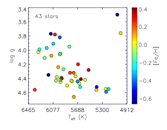
Figure 1: Parameter space covered by the sample stars. The values are listed in Table 1.

2.2 do Pico dos Dias observations

We used coudé and MUSICOS in 2016 and 2017. Both spectrographs are fed by the 1.60 m Perkin-Elmer telescope of do Pico dos Dias Observatory (OPD, Brazópolis, Brazil), operated by Laboratório Nacional de Astrofısica (LNA/CNPq). In the coudé spectrograph the slit width was adjusted to give a two-pixel resolving power $R=\lambda/\Delta\lambda=45\,000$. A 1800 l/mm diffraction grating was employed in the first order, projecting onto a 13.5 $\mu$m, 2048 pixels CCD. The spectral region is centered on the H$\alpha$ line $\lambda=6562.797$ Å, with a spectral coverage of $155$ Å.

MUSICOS is a fiber-fed echelle spectrograph (e.g. Baudrand & Bohm 1992) (on loan from Pic du Midi Observatory since 2012) available for the OPD/LNA. We employed the red channel, covering $\lambda$5400-8900 Å approximately, comprising about 50 spectral orders, at R $\sim 40\leavevmode\nobreak\ 000$ and 0.05 Å/pix dispersion in the H$\alpha$ wavelength range.

The exposure times were chosen to obtain S/N ratios of at least 250 for the faintest stars ($V\sim 7$) and 300 in average for the other stars.

3 Normalization

The challenge in normalizing H$\alpha$ profiles arises from the uncertainty of the continuum location, that is estimated defining “continuum windows”. Thus, the success of the normalization resides in the capability of identifying many wide windows that allow to determine the shape of the spectrograph response.

Frequently, the continuum windows are determined using automatic or semiautomatic procedures, as the IRAF task “continuum”, selecting the wavelength bins with the highest fluxes by applying clipping. We improve this procedure by iterating on the normalization and fitting processes, in this way the compatibility at the extremes of the wings are checked after every fit. This check is fundamental for consistent temperature measurements because, although the spectrograph response may be well described by a low order polynomial (as is the case of coudé), the normalization by interpolation may be highly imprecise close to the line-core. It occurs because the continuum regions available to interpolate the polynomial are short compared to the fitted region, thus small errors in the outer profile wings trigger larger errors close to the line-core, where the H$\alpha$ profile is more sensitive to the temperature. With this method, explained below in detail, we minimize the main source of uncertainty, as demonstrated by the very low dispersion of $T_{\mathrm{eff}}^{\mathrm{H}\alpha}$ values obtained with many solar spectra in Sect. 6.1 and 10.

Normalization is more complex in echelle spectra, because of the correction of the blaze and order merging. As discussed by Škoda & Šlechta (2004), distortions in the spectra, such as discontinuities of the orders and ripple-like patterns (see Škoda et al. 2008, Fig. 11) are often produced in slit echelle spectrographs but possibly also in fiber-fed instruments. When this occurs, the spectra are useless and a new reduction from raw data should be applied following the recipe recommended by Škoda et al. (2008). Of course, empirical corrections on the reduced spectra could recover the profiles, but their goodness must be tested by recovering the $T_{\mathrm{eff}}$ accuracy obtained with non-distorted profiles. On the other hand, also spectra with no obvious distortions need to be tested, because subtle residual blaze features may remain and systematically impact the $T_{\mathrm{eff}}$ estimate. Residual blaze features distort the profiles making them shallower (more strongly close to the center of the spectral order), thus the distorted spectra mimic profiles of cooler temperatures. In order to investigate this effect in HARPS, the 1D pipeline-reduced HARPS spectra were analyzed in the same way as the coudé ones, and the derived $T_{\mathrm{eff}}^{\mathrm{H}\alpha}$’s were compared. The results of this analysis are presented in Sect. 10.

The normalization method applied to coudé and HARPS is independently validated by deriving $T_{\mathrm{eff}}^{\mathrm{H}\alpha}$’s from MUSICOS spectra normalized with the 2D-normalization. These results are presented in Sect. 5.

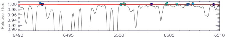
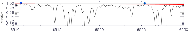
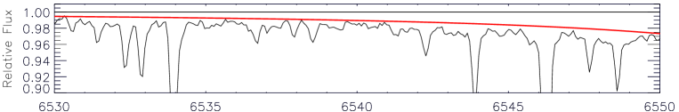
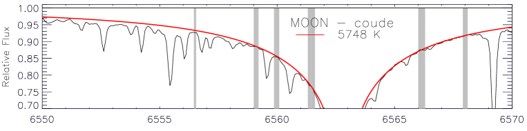
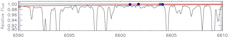
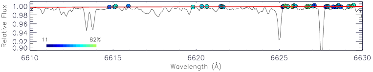
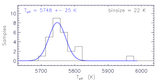
Figure 2: Coudé H$\alpha$ profile of one of the solar proxies in Table 3. The red and black lines represent the synthetic and observed profiles. The shaded regions are the windows of fits and the circles represent the continuum bins color-coded according to their frequency of appearance in all coudé spectra. The most frequent continuum windows are observed at [6500.25, 6500.50], [6504.50, 6505.00], [6619.70, 6620.50], [6625.60, 6625.80] and [6626.50, 6626.80]. Bottom panel: Histogram of temperatures related to the wavelength bins within the windows of fits. A Gaussian is fitted to its median and robust standard deviation.

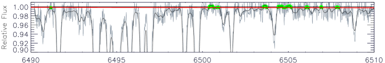
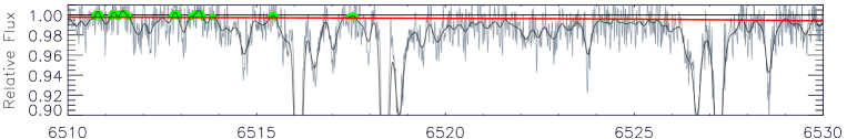
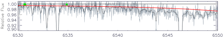
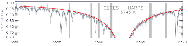
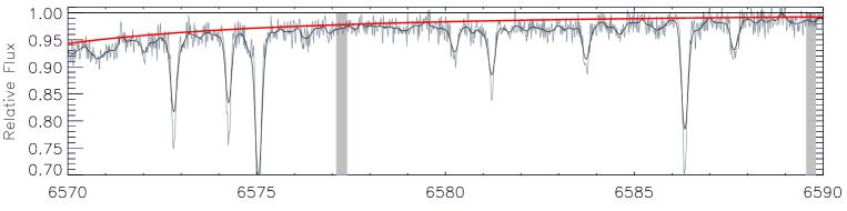
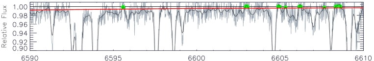
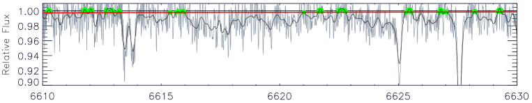
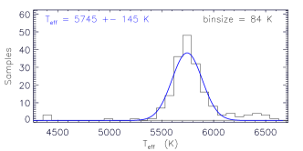
Figure 3: Analogous to Fig. 2 with a HARPS spectrum of one of the solar proxies from Table 3. The gray line represents the spectrum in its original resolution and the black line represents the spectrum degraded to the resolution of coudé. Continuum bins in the degraded spectrum are highlighted in green; notice that they mostly match those of Fig. 2.

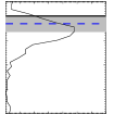
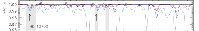
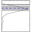
Figure 4: Left panels: Fitting of two coudé spectra (gray line) with synthetic spectra of PWV with concentrations of 10 and 20 mm (red and blue lines). The circles are the continuum wavelength bins on 1 $\pm\leavevmode\nobreak\ \sigma$(noise). The shades represent 3 of the 5 continuum windows selected in Fig. 2. The arrows point the windows contaminated by telluric features. Right panels: Flux histograms of the spectra on the left panels with the same flux scale. The black horizontal line points the continuum, the dashed line is the average flux of the 5 continuum windows of Fig. 2 and the shades are the spread.

3.1 Normalization of coudé and HARPS spectra

The normalization is applied by interpolating low order polynomials with the IRAF task “continuum”, integrated with the fitting code described in Sect. 5 in an iterative procedure:

1. A first gross normalization is performed neglecting the region $6514-6610$ Å in the interpolation. Although the extension of the H$\alpha$ wings is variable, this region is kept the same for all the sample stars with the purpose of keeping enough room to apply weights in nearby regions to modulate the normalizing curve.

2. The obtained profile is used to fit a precipitable water vapor (PWV) spectrum that will be used to verify the continuum level after every iteration, see Sect. 3.2.

3. The same normalized profile is compared with the grid of synthetic profiles using the fitting code described in Sect. 5 to find the most compatible one.

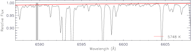
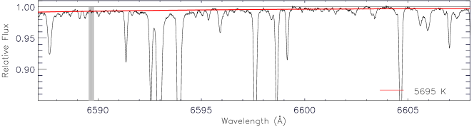
Figure 19: From the top to the bottom, transition regions at the red wing in fitted coudé, KPNO2005, and KPNO2011 spectra. The panel in the top is related to the spectrum in Fig. 2, and the two panels below are related to the spectra in Fig. 18.

4. The compatibility between the normalized and synthetic profiles must be visually checked at the “transition regions” ($\lambda<6536$ Å and $6590$ Å ¡ $\lambda$) in which the continuum turns into line wings. The regions of the line interior are very sensitive to temperature, hence they are predominant in the fittings. For this reason, if distortions are artificially introduced in the profile during the normalization, they become more evident in the transition regions. This procedure makes our normalizations dependent on the model but very weakly, because metallicity and surface gravity (the parameters set beforehand) do not greatly influence the shape of the line, especially in the transition regions. We verified that changes as large as $\sim\!\!\pm 0.3$ dex do not modify significantly the shape of the normalized profiles, while larger changes may truncate the procedure. For consistency, HARPS spectra were degraded to the resolution of coudé in this step (only for this step, not for the fitting procedure), see Fig. 3. In Fig. 19 examples of transition regions at the red wing of H$\alpha$ in solar spectra normalized by different authors are provided. In it, the fit of the coudé spectrum of Fig. 2 is compared with fits of KPNO2005, and the solar atlas of Wallace et al. (2011) (KPNO2011) to show how this method improves the normalization.

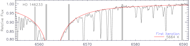
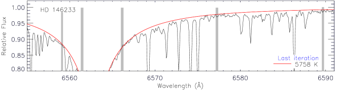
Figure 21: Results from the iterative H$\alpha$ normalization-fitting of one of the two coudé spectra of 18Sco (HD 146233) following the procedure described in Sect. 3.1.

5. Usually the first normalization is deficient, in this case a second one is performed from scratch applying weights to the wings around 6514 and $6610$ Å to make the profile deeper or shallower as required to match the flux of the synthetic profile. Then, another fit is applied and the matching check described in step 4 is repeated. The procedure finishes when the observed and synthetic profiles are compatible in the transition regions, as shown in Fig. 2 and 3. An example of the difference between the first gross normalization and the final normalization is shown in Fig. 21.

3.2 Continuum fine-tune

The solar KPNO2005 atlas and the lines catalog of Moore et al. (1966) were used to select windows free from metallic lines to check the continuum during the normalization procedure. However, the availability of these windows diminish progressively in cool and metal-rich stars and because of the presence of telluric lines. Since the humidity at do Pico dos Dias Observatory often exceeded $90\%$ during our observations, the contribution of many minute telluric lines is relevant in the coudé spectra. To fine-tune the continuum level, as part of the procedure described in Sect. 3.1, we separated telluric features from noise fitting the observed spectra with synthetic telluric spectra as shown in Fig. 4.

Attempts for the fittings were performed with the Molecfit software package described in detail in Sect. 4.1 and with the PWV library of Moehler et al. (2014). The first demonstrated to be precise for fitting strong features but many more weak features are present in the second, which makes it more suitable for this analysis. The PWV library is available at resolutions R = 300 000 and R = 60 000, for the air-masses 1.0, 1.5, 2.0, 2.5, 3.0 and water content of 0.5, 1.0, 1.5, 2.5, 3.5, 5.0, 7.5, 10.0, and 20.0 mm. The fitting is performed degrading the resolution of the original PWV spectra to match those of the spectrograph used, and selecting the set of PWV spectra with the air-mass closest to that of the observation.

We quantified the displacement of the continuum due to the presence of telluric features as follows. After normalized all coudé spectra, continuum wavelength bins were identified in the solar spectrum of Fig. 2 applying $\sigma$-clipping. The fluxes of these wavelength bins were then checked in all other normalized coudé spectra, and none of them was found to remain as continuum in all the sample. The color-code of the plot in the figure represents the percentage rate, being the windows at [6500.25, 6500.50], [6504.50, 6505.00], [6619.70, 6620.50], [6625.60, 6625.80], [6626.50, 6626.80] Å the most frequent. Fig. 4 shows two cases where two of these windows are affected by the presence of minute telluric lines, and how much the average flux of the five mentioned windows decreases. Analyzing all the sample spectra, we find that when the content of PWV is high, say between 7.5 and 20.0 mm, minute telluric features are almost omnipresent and displace the continuum flux by about $0.5\%$. In our experience, this issue may induce to underestimate the stellar temperature between 30 and 100 K. It is however difficult to provide a precise estimate because the displacement produced is often not homogeneous, but a distortion of the continuum shape. We stress that no correction is applied during this procedure, only a visual check. The correction of strong features is done later, and it is explained Sect. 4.1.

4 Profiles fitting

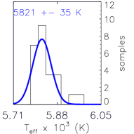
Figure 5: Telluric correction and profile fitting of the coudé spectrum of HD 2151. Left panel: Corrected and non corrected spectra are represented by the black and blue lines, respectively. The windows of fits are represented by the shades, and the arrows point those where the relative flux was perfectly recovered. The red line represent the synthetic profile fitted. Right panel: Histogram of temperatures related to the wavelength bins inside the windows of fits. The most probable $T_{\mathrm{eff}}^{\mathrm{H}\alpha}$ is shown in the top part of the plots, also log log g and [Fe/H] values used for the fittings along with their source in the literature are shown.

This study is based on the grid of synthetic profiles of BPO02 computed using the self-broadening theory developed in Barklem et al. (2000) and the 1D LTE plane-parallel model atmospheres from the MARCS code (Asplund et al. 1997). The atmospheric parameters of the grid are $T_{\mathrm{eff}}$: 4400 to 7500 K with steps of 100 K, [Fe/H]: $-3.0$ to $+0.5$ dex with steps of 0.5 dex, log g: 3.4 to 5.0 dex with steps of 0.5 dex and microturbulence velocity of 1.5 Km$/$s. In order to derive very precise $T_{\mathrm{eff}}$’s around solar parameters, a more detailed grid from the same theoretical recipe used by Ramírez et al. (2011) (kindly provided by the first author by private communication) is also used here, its parameters are $T_{\mathrm{eff}}$: 5500 to 6100 K with steps of 10 K, [Fe/H]: $-3.0$ to $+0.3$ dex with steps of 0.05 dex, log g: 4.2 to 4.65 dex with steps of 0.05 dex and microturbulence velocity of 1.5 Km$/$s. The fitting between the observed and synthetic profiles is performed using the “windows of fits” free from metallic lines: [6556.45, 6556.55], [6559.00, 6559.20], [6559.86, 6560.08], [6561.30, 6561.60], [6566.00, 6566.30], [6567.90, 6568.10], [6577.10, 6577.40], [6589.55, 6589.80].

A program in IDL was written to perform the fits eliminating the influence of contaminated wavelength bins. It first interpolates the resolution of the grids to 1 K, 0.01 dex, 0.01 dex in $T_{\mathrm{eff}}$, [Fe/H], log g. Then, for each wavelength bin, the temperature related to the interpolated synthetic profile with the closest flux value is chosen, [Fe/H] and log g previously fixed by the user. The most probable temperature and its uncertainty are determined by the median and the robust standard deviation (1.4826 times the median absolute deviation) of the histogram, see e.g. Fig. 2 and 3.

4.1 Telluric correction

The resolution and sampling of the coudé spectra allow a total of 26 to 27 wavelength bins inside the windows of fit, enough to perform the fitting procedure described in Sect 5. In order to optimize $T_{\mathrm{eff}}^{\mathrm{H}\alpha}$ and its error determination when windows of fits are contaminated and to provide a spectral library clean from telluric features, we corrected the normalized coudé spectra with the Molecfit software package (Smette et al. 2015; Kausch et al. 2015). This software computes the transmission of the Earth’s atmosphere at the time of the observations with the radiative transfer code LBLRTM (Clough et al. 2005), taking into account spectroscopic parameters from the HITRAN database (Rothman et al. 2013) and an atmospheric profile. The atmospheric transmission is fitted to the observed spectrum, and the telluric correction is done dividing the observed spectrum by the atmospheric transmission. We used the average equatorial atmospheric profile, which is Molecfit’s default profile. We chose to fit H₂O (the main absorber in this wavelength region), O₂, and O₃. The line shape is fitted by a boxcar profile; as starting value for the boxcar FWHM we used 0.36 times the slit width. The wavelength solution of the atmospheric transmission is adjusted with a first degree polynomial. First, we ran Molecfit automatically on all spectra, avoiding the center of the H$\alpha$ line from 6560 to 6566 Å. If the residuals of this first telluric correction were larger than 2% of the continuum, we adapted the starting value of the water abundance and performed a second fit. This telluric correction allowed us to recover with precision the stellar flux inside the contaminated windows of fits in most cases. An example is shown in Fig 5 where the corrected and non-corrected spectra of HD 2151 are over-plotted.

The telluric corrected and non-corrected normalized coudé spectra of the sample stars in Table 1 can be accessed at an on-line repository, or by contacting the first author.

5 Validation of the normalization method

BPO02 found the 2D-normalization efficient in removing the spectral blaze, the method is described in detail in their paper. It is referred as 2D-normalization because it depends on the two spacial dimensions of the CCD detector. Namely, the normalization curve of the spectral order of interest is found by interpolating the normalization curves of the adjacent orders in the pixel domain.

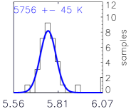
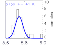
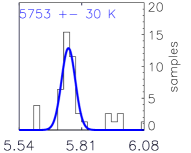
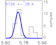
Figure 17: Profile fits of MUSICOS solar spectra.

We validate the normalization method described in Sect. 3.1 used on coudé and HARPS spectra, deriving $T_{\mathrm{eff}}^{\mathrm{H}\alpha}$ with MUSICOS spectra normalized by the 2D-normalization. The comparison in Fig. 6 shows that $T_{\mathrm{eff}}^{\mathrm{H}\alpha}$ derived with coudé and MUSICOS are compatible for all stars.We find no trend with respect to the atmospheric parameters, a negligible offset of $-1$ K and a low scatter of 25 K. Solar spectra reflected in the Moon and Ganymede were also normalized with this method, from which we derive the average value $5745\pm 16$ K (see comparative values in Table 3, the profile fits are shown in Fig. 17) consistent with $T_{\mathrm{eff}}^{\mathrm{H}\alpha}$’s listed in Table 2 derived from coudé and HARPS spectra.

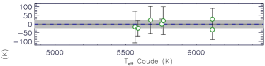
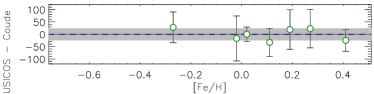
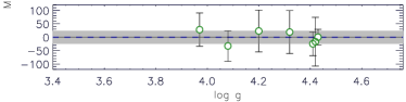
Figure 6: Temperature diagnostics from MUSICOS with respect to those of coudé vs. atmospheric parameters. [Fe/H] and log g values from Table 1 were used here. The $-1$ K offset and its 25 K scatter are represented by the dashed lines and the shades, respectively.

6 Accuracy of 1D model atmospheres

6.1 The zero-point

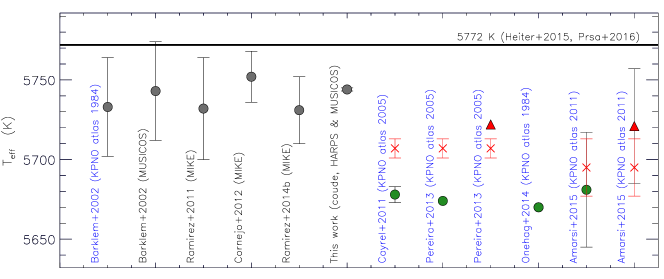
Figure 7: Graphic representation of solar $T_{\mathrm{eff}}$ values in Table 2. The horizontal line represents the solar $T_{\mathrm{eff}}$ measured by the Stefan-Boltzmann equation. Works that used theoretical models based on 1D atmosphere models are represented by circles, and those that used 3D models by triangles. Gray circles represent works that used the theoretical model of BPO02, and green circles represent a different/enhanced recipe. Works that used KPNO solar atlases are labeled in blue. For them, for comparison purposes, our measurements from corresponding KPNO spectra are included as red crosses in the same line.

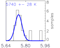
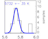
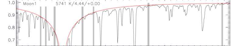
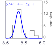
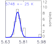
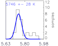
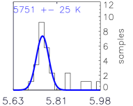
Figure 16: Profile fits of coudé solar spectra.

We used the 6 blaze-free coudé solar spectra listed in Table 3 to determine the accuracy of H$\alpha$ profiles from 1D model atmospheres for the Sun. The profiles fitted are shown in Fig. 16, we obtain the average value $5744\pm 7$ K. Since we find good agreement between the determinations from coudé, MUSICOS, and HARPS spectra (Sec. 5 and 10), we determine the zero-point of the model by averaging the inferred $T_{\mathrm{eff}}$ values from all solar spectra, resulting an offset of $-28\pm 1$ K with respect to the 5772 K (Prša et al. 2016; Heiter et al. 2015) measured by the Stefan-Boltzmann equation.

Our zero-point supports the temperature values initially found by BPO02 with their MUSICOS spectrum and the KPNO1984 atlas, and those found later by Ramírez et al. (2011); Cornejo et al. (2012) and Ramírez et al. (2014b) with MIKE spectra. On the other hand, it disagrees with any value derived from KPNO solar atlases, including our own determinations. These values are presented in Table 2 and Fig. 7 along with those derived by other authors using enhanced theories from BPO02 on.

Fig. 7 shows that none of the models recovered the solar $T_{\mathrm{eff}}$, included the most sophisticated ones, i.e. Pereira et al. (2013) based on 3D models and Amarsi et al. (2018) based on 3D models and NLTE conditions. The plot also shows that the determinations from KPNO spectra are systematically cooler than those from other spectra, except for the first one of BPO02. Notice that this determination disagrees with that of Önehag et al. (2014) although they were obtained with the same version of KPNO atlas and the same broadening recipe. Which is explained by synthetic profiles computed from different versions of MARCS model atmospheres that use distinct mixing-length parameters.

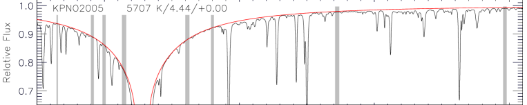
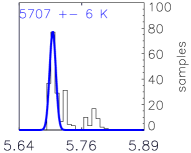
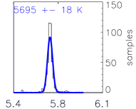
Figure 18: Profile fits of KPNO2005 (top), and KPNO2011 (bottom) spectra.

It is not satisfactory that such dispersion remains for the Sun, our reference star from which spectra of supreme quality are not difficult to obtain. Thus, in the attempt of identifying the origin of the problem, we fitted KPNO atlases with the theoretical profiles of BPO02 (fittings with no further normalization). From these fits, we firstly computed the temperature difference that other models of H$\alpha$ produce with respect to that of BPO02 for the Sun, they are provided in Table 2. Secondly, we compared these fits with those of coudé/HARPS/MUSICOS to analyze the goodness of their normalizations. The fits are shown in Fig. 18, they are very precise in the inner profile regions thanks to their high temperature sensitivity and to the high spectral quality in S/N and sampling. However, when the outer regions are scrutinized, evident departures appear, see Fig. 19. We observed similar departures, after the first iteration in our normalization procedure, i.e. the custom normalization by polynomial interpolation (see Fig. 21), whose causes were explained in Sect. 3.

From KPNO2005 we obtain a 30 K cooler value than what we obtain with coudé/HARPS/MUSICOS spectra. This atlas version was normalized by polynomial fitting of the observed spectral fluxes, considering also the presence of broad $\mathrm{O_{3}}$ and $[\mathrm{O_{2}}]_{2}$ atmospheric features produced by synthetic spectra. The differences between the temperature values derived by us and the two authors that used profiles from 1D models are entirely explained by the different physics of the models. H$\alpha$ profiles of Cayrel et al. (2011) were synthesized by ATLAS9, BALMER9 codes (Castelli & Kurucz 2004) and the impact-broadening of Allard et al. (2008) that includes more transitions than the self-broadening of BPO02. The profiles of Pereira et al. (2013) were synthesized also with a slight different input physics and an updated atmosphere model than that in BPO02.

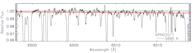
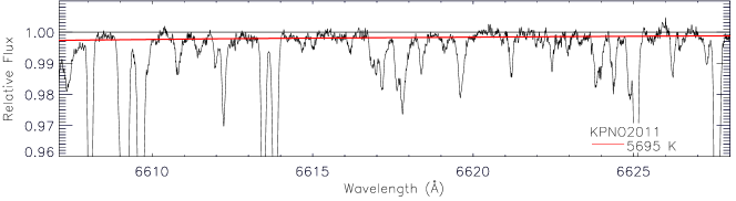
Figure 20: For the KPNO2011 atlas, spectral regions that contain the continuum windows [6500.25, 6500.50] and [6504.50, 6505.00] (top), and [6619.70, 6620.50], [6625.60,6625.80] and [6626.50, 6626.80] (bottom).

From KPNO2011 we obtain a similar value to that obtained with KPNO2005, meaning that the relative flux of both spectra in the innermost regions of the profile agree. On the other hand, significant differences are observed in the outer wings, see Fig. 19. No information is provided about the normalization method of this atlas, but we suspect that the custom method was applied because we observe significant flux disparities around the continuum regions [6500.25, 6500.50], [6504.50, 6505.00] and [6625.60, 6625.80], see Fig. 20. If their flux excess of $\sim\!0.2\%$ was constant through all the wavelength range, it would imply a temperature underestimate of at least 20.

This analysis show that the systematic low temperatures from solar spectra in Table 2 are associated to disparities with the synthetic spectra and/or the continuum, which may indicate minute normalization errors. We show that when a special care is taken in the continuum placement and in fitting the outermost profile regions, consistent results are obtained. These results are further supported by the agreement with all other $T_{\mathrm{eff}}^{\mathrm{H}\alpha}$ measurements from spectra other than KPNO, as Fig. 7 shows.

The temperature differences listed in the last column of Table 2 are computed subtracting the diagnostics by the BPO02 model to those by the H$\alpha$ models of the authors listed in the first column, both obtained from the same solar spectra listed in second column. Hence, they give the zero-points of the H$\alpha$ models relative to that of BPO02 ($-28\pm 1$ K), so the two quantities added give the zero-point of the model. Remarkably, we find that the two models using 3D atmospheric models improve the agreement with the actual solar $T_{\mathrm{eff}}$, and Amarsi et al. (2018) that also consider NLTE reproduce almost exactly the solar $T_{\mathrm{eff}}$.

Table 2: Third column lists $T_{\mathrm{eff}}$ values derived for the Sun with H$\alpha$ profiles from 1D model atmospheres (top table) and from 3D model atmospheres (bottom table). Forth column lists the temperature differences given by different models of H$\alpha$ with respect to BPO02-grid based analysis for the same solar spectrum. Fits of the spectra are shown in the appendix.

Author	spectrum	$T_{\mathrm{eff}}$ (K)	$\Delta$$T_{\mathrm{eff}}$ (K)
BPO02	KPNO1984	$5733$	—
BPO02	MUSICOS	$5743$	—
Ramírez et al. (2011)	MIKE	$5732\pm 32$	—
Cayrel et al. (2011)	KPNO2005	$5678\pm 5$	$-29$
Cornejo et al. (2012)	MIKE	$5752\pm 16$	—
Ramírez et al. (2014b)	MIKE	$5731\pm 21$	—
Pereira et al. (2013)	KPNO2005	$5674$	$-33$
Önehag et al. (2014)	KPNO1984	$5670$	—
Amarsi et al. (2018)	KPNO2011	$5681\pm 40$	$-14$
This work	coudé	$5744\pm 7$	—
This work	HARPS	$5744\pm 10$	—
This work	MUSICOS	$5745\pm 16$	—
This work	KPNO2005	$5707\pm 6$	—
This work	KPNO2011	$5695\pm 18$	—
Pereira et al. (2013)	KPNO2005	$5722$	15
Amarsi et al. (2018)	KPNO2011	$5721\pm 40$	26

6.2 Accuracy for non solar stars

Atmospheric parameters of 34 Gaia Benchmark stars with a wide range of temperature and metallicity were published by Heiter15. Their $T_{\mathrm{eff}}$’s were derived by measuring angular diameters with interferometry, that is the least model-dependent technique. We acquired coudé spectra of 9 Gaia Benchmark stars and $T_{\mathrm{eff}}^{\mathrm{H}\alpha}$ were derived for them using the [Fe/H] and log g values given by the authors. The plot in Fig. 8 shows the comparison of $T_{\mathrm{eff}}^{\mathrm{H}\alpha}$ with $T_{\mathrm{eff}}$ from interferometry. We find a constant offset of 30 K between the two scales, that confirms the $-28$ K zero-point found with the solar spectra in Sect. 6.1. No temperature dependence is found with log g but a trend is present with metallicity. The right panel of the figure shows that H$\alpha$ underestimates $T_{\mathrm{eff}}$ by $\sim\!100$ K at [Fe/H] = $-0.5$. In the plots, the temperature values of $\mu$ Ara (HD 160691) appear highly discrepant and were ignored to compute the trend. Its interferometric $T_{\mathrm{eff}}$ is flagged by the authors as not reliable because its angular diameter is not directly measured (see Sect. 3.2 in paper); also its mass measurements derived by evolutionary and seismic techniques disagree. On the other hand, we find its $T_{\mathrm{eff}}^{\mathrm{H}\alpha}$ to be consistent with IRFM and all the spectroscopic values in following sections. The other star with a high discrepancy is $\delta$ Eri (HD 23249). It appears also discrepant in the comparison with IRFM in Sect. 7.1, and even our temperatures from coudé and HARPS disagree. However, its values in the plots of Fig. 8 were not ignored at computing the trends, in order to do an homogeneous comparison with the trends in Fig. 9.

Having determined with high precision the offset of $T_{\mathrm{eff}}^{\mathrm{H}\alpha}$ with respect to $T_{\mathrm{eff}}$ at solar parameters in the previous subsection, the $T_{\mathrm{eff}}^{\mathrm{H}\alpha}$ accuracy with respect to [Fe/H] over the metallicity range analyzed, is improved from the relation in the plot on right panel of Fig. 8 to $T_{\mathrm{eff}}=T_{\mathrm{eff}}^{H\alpha}$ $-159(\pm 80)$[Fe/H] $+28(\pm 1)$ K (68 K scatter).

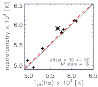
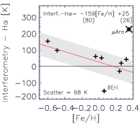
Figure 8: Left panel: Comparison of $T_{\mathrm{eff}}^{H\alpha}$ with $T_{\mathrm{eff}}$ from interferometry of the Gaia Benchmark stars (Heiter15). The red dashed line represent the offset. Right panel: Relative temperatures in function of [Fe/H]. The red line and the shade represent the trend and its scatter. The corresponding function and the errors of its coefficients (in brackets) are shown in the legends. The cross symbol in both plots point $\mu$ Ara’s (HD 160691) considered as outlier.

7 Consistency with other $T_{\mathrm{eff}}$ scales

We used 10 catalogs from literature to determine the consistency of the H$\alpha$ profile diagnostics with other techniques. Among them, Sousa08, Ghezzi10, Tsantaki13, Besnby14, Ramirez14a, Ramirez14b, and Maldonado15 determine spectroscopic $T_{\mathrm{eff}}$’s, while Ramirez13 has $T_{\mathrm{eff}}$’s derived by photometric calibrations from IRFM.

In this section, as well in Sect. 6.2, $T_{\mathrm{eff}}^{\mathrm{H}\alpha}$’s were derived for comparison purposes using as stellar imput log g and [Fe/H] parameters provided by each author, so that the comparisons are consistent as far as the stellar parameters are concerned. In the next subsections $T_{\mathrm{eff}}^{\mathrm{H}\alpha}$ determinations are separately compared with the results obtained with each method.

7.1 IRFM effective temperatures

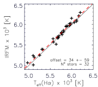
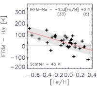
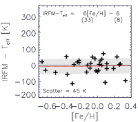
Figure 9: Left and middle panels: Same as in Fig. 8 for the $T_{\mathrm{eff}}^{IRFM}$’s of Ramirez13. Right panel: Relative temperatures in function of [Fe/H] after applying the correction relation given in 6.2 to $T_{\mathrm{eff}}^{\mathrm{H}\alpha}$.

The comparison with IRFM is performed with the temperatures of Ramirez13, that were derived by the metallicity-dependent color–$T_{\mathrm{eff}}$ calibrations of Casagrande et al. (2010) using the Johnson-Cousins, 2MASS, Tycho2 and Strömgreen available photometry. To obtain these temperatures, represented by $T_{\mathrm{eff}}^{IRFM}$, the authors used an homogeneous set of metallicity derived from Fe lines, where $T_{\mathrm{eff}}$ is not obtained simultaneously with the other parameters but fixed from photometric calibrations. In this way, both techniques are combined iteratively minimizing the $T_{\mathrm{eff}}$–[Fe/H] degeneracy.

The plot in Fig. 9 shows the comparison between $T_{\mathrm{eff}}^{IRFM}$ and our coudé $T_{\mathrm{eff}}^{\mathrm{H}\alpha}$. There is a constant offset of +34 K between the two scales with a 59 K scatter. Their difference show a trend with metallicity according to the equation displayed in the plot on the middle panel. This trend is practically the same found in the comparison with interferometric measurements, asserting the equivalence of the two scales (Casagrande et al. 2014). After applying the relation given in Sect. 6.2 to $T_{\mathrm{eff}}^{\mathrm{H}\alpha}$, the trend is indeed fully removed, as shown in the right panel of the figure. The remaining 45 K scatter is close to the average formal errors of $T_{\mathrm{eff}}^{IRFM}$ of the stars compared (52 K), which implies that it is dominated by the uncertainties of the color measurements. Therefore the contribution of random errors of $T_{\mathrm{eff}}^{\mathrm{H}\alpha}$ related to the normalization is negligible, supporting the precision of our method.

7.2 Spectroscopic effective temperatures

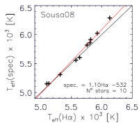
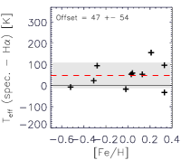
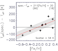
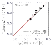
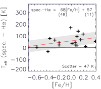
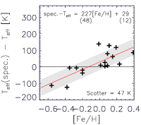
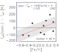
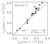
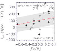
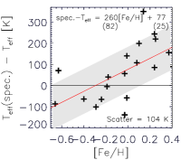
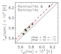
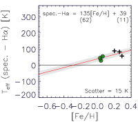
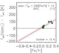
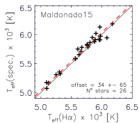
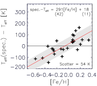
Figure 10: Same as in Fig. 9 for spectroscopic $T_{\mathrm{eff}}$’s. The authors are indicated in the plots on the left panels. In all plots, the black lines represent the prefect agreement and the red lines the trends. When the trends are found not significant, the offsets are drown with dashed red lines. $T_{\mathrm{eff}}$’s from Ramirez14a (plus symbols) and Ramirez14b (green circles), derived with the same method, are compared in the same plots.

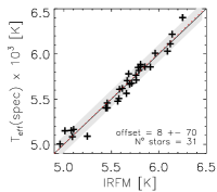
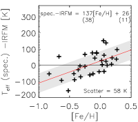
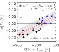
Figure 11: Left and middle panels: Similar to Fig. 8 for the $T_{\mathrm{eff}}^{IRFM}$’s of Ramirez13 against the spectroscopic $T_{\mathrm{eff}}$’s of Sousa08. Right panel: $\Delta$[Fe/H] represent the metallicity values of Sousa08 with respect to those of Ramirez13. The blue symbols are the stars with over-solar $T_{\mathrm{eff}}$’s.

The need of deriving accurate stellar atmospheric parameters got more attention with the discovery of exoplanets, because their characterization depends directly on how accurately and precisely the physical parameters of the host stars are known. Other studies also require a refined determination of $T_{\mathrm{eff}}$, for instance, finding the nature of the connection between stellar metallicity and planetary presence (e.g. Santos et al. 2003; Fischer & Valenti 2005; Sousa et al. 2008; Ghezzi et al. 2010), the detection of diffusion effects in the stellar atmospheres (e.g. Korn et al. 2006, 2007) and the search for chemical signatures of planetary formation (e.g. Meléndez et al. 2009; Ramírez et al. 2009). Some of them deal with a large amount of stars, for which automatic spectroscopic procedures have been developed, that provide results with high internal precision. However, as shown by Ryabchikova et al. (2015) in their Fig. 1, when results from different spectroscopic procedures are compared, significant discrepancies may appear.

In this work we considered for comparison catalogs with small internal errors. Among them Ramirez14a and Ramirez14b are the most precise with $\sim\!10$ K. They are followed by Sousa08, Tsantaki13 and Maldonado15 with $\sim\!20$ K, a bit further Ghezzi10 and Heiter15 with $\sim\!30$ K and Bensby14 $\sim\!70$ K. The plots in Fig. 10 show the comparison of our temperature determination from coudé with those derived by the different sources.

Sousa08, Ghezzi10 and Tsantaki13: all derive $T_{\mathrm{eff}}$ assuming LTE and 1D geometry by the Kurucz Atlas 9 (Kurucz 1993) model atmospheres. They used the 2002 version of MOOG (Sneden 1973) and the ARES code for automatic measurement of equivalent widths (Sousa et al. 2007). They differ in the line-lists used and in the atomic data adopted. Tsantaki13’s line-list is an upgrade of the Sousa08’s list selected with HARPS, where “bad” lines were suppressed to correct $T_{\mathrm{eff}}$ overestimate in cooler stars. Both works computed log gf values from an inverted solar analysis using equivalent widths measured in solar spectra. Ghezzi10’s list is short in comparison with those of Sousa08 and Tsantaki13, it was selected for the FEROS spectrograph (Kaufer et al. 1999) at lower resolution; the log gf they used are obtained in laboratory. The comparison with these three works show a trend with $T_{\mathrm{eff}}^{\mathrm{H}\alpha}$: the larger $T_{\mathrm{eff}}$, the larger is the discrepancy. For Ghezzi10, the comparison between our measurements and theirs show a positive trend with [Fe/H], while for Sousa08 and Tsantaki13 no trend with [Fe/H] is found, but offsets of 48 and 33 K, respectively.

Bensby14: derived $T_{\mathrm{eff}}$ considering NLTE corrections on spectral lines measured manually. The 1D MARCS model atmospheres (Asplund et al. 1997) were used with an own code of convergence of atmospheric parameters. They used a large line-list and spectra from different instruments of medium and high resolution, with log gf values obtained in laboratory. The comparison of their $T_{\mathrm{eff}}$ scale against $T_{\mathrm{eff}}^{\mathrm{H}\alpha}$ is similar to those of Sousa08 and Tsantaki13. Indeed, Sousa08 find their scale to be compatible to an offset of $+18$ K respect Bensby14’s (see Fig. 3 in paper). We find a slightly significant positive trend with [Fe/H].

Ramirez14a and Ramirez14b: used a differential method (Meléndez et al. 2006) with which the atmospheric parameters of high internal precision are obtained. By means of the “$\textit{q}^{2}$” package both groups of authors used the 2013 version of MOOG and 1D-LTE model atmospheres grids. They, measured spectral lines manually and used atomic data from laboratory. There are two main differences between the procedures of Ramirez14a and Ramirez14b. Firstly, Ramirez14a used the “odfnew” version of Kurucz, while Ramirez14b used MARCS atmosphere model (Gustafsson et al. 2008). However, according to Ramirez14b the use of different models does not affect significantly the parameters diagnostics because of the differential method applied. Secondly, the stars analyzed in both works differ in [Fe/H]: Ramirez14b analyzed solar twins, while Ramirez14a more metal-rich stars, i.e. [Fe/H] $\gtrsim 0.2$. Thus, Ramirez14b naturally used the Sun as standard for the solar twins, while in Ramirez14a the differential method was applied respect every star of the sample. For the Ramirez14b’s scale of solar twins we find an offset of $+42\pm 13$ K respect H$\alpha$, which agrees with the $28\pm 1$ K needed to correct H$\alpha$ zero-point. For the Ramirez14a’s scale we find an offset of $+72\pm 17$. Considering Ramirez14a and Ramirez14b a unique sample, we find a positive trend with [Fe/H].

Maldonado15: assumed LTE and 1D geometry by the Kurucz Atlas 9 model atmospheres as Sousa08, Ghezzi10, and Tsantaki13, but they used the line-list from Grevesse & Sauval (1999) and spectra from several sources including HARPS. For the convergence of the atmospheric parameters they used TGVIT (Takeda et al. 2005). The comparison of their $T_{\mathrm{eff}}$ scale against H$\alpha$ does not show a significant trend, but an offset of +34 K. We found the same offset for IRFM against H$\alpha$ (Sect. 7.1), which confirms the agreement between this $T_{\mathrm{eff}}$ scale and IRFM reported by the authors. On the other hand we find a positive trend with [Fe/H].

The spectroscopic scales analyzed in this section show, in general, agreement with H$\alpha$ up to $\sim\!\!5700$ K and hotter diagnostics for hotter $T_{\mathrm{eff}}$’s. The trends with [Fe/H] are opposite to that we observe with interferometry and IRFM. After applying the correction relation for metallicity of Sect. 6.2 to $T_{\mathrm{eff}}^{\mathrm{H}\alpha}$, the H$\alpha$ scale can be considered in the same frame of the interferometry scale, allowing to study the accuracy of the spectroscopic scales. This is shown in the right panels of Fig. 10, the common pattern shows that spectroscopic temperatures are underestimated by 100-200 K at [Fe/H] = $-0.6$ dex and overestimated by $\sim\!\!100$ K at [Fe/H] = $+0.4$ dex. The most accurate [Fe/H] range is around the solar value, say between $-0.3$ and $+0.1$ dex.

The relations presented in the plots can be used to empirically correct spectroscopic scales. These corrections become important as $T_{\mathrm{eff}}$ depart from solar, to derive unbiased [Fe/H] values. An example of the impact of the $T_{\mathrm{eff}}$ scale on [Fe/H] is provided in Fig. 11. The plots compare the temperature and metallicity scales of Sousa08 and Ramirez13. No offset between both temperature scales appears, but their difference plotted against [Fe/H] replicate the trend obtained in the top right panel of Fig. 10. The difference between metallicity scales also shows a trend with $T_{\mathrm{eff}}$, associating larger [Fe/H] discrepancies with $T_{\mathrm{eff}}$ farther from solar.

8 Comparison with other H$\alpha$ scales

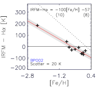
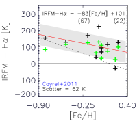
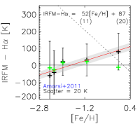
Figure 12: From left to right, analogous comparisons to the middle panel in Fig. 9 for the H$\alpha$ scales of BPO02, Cayrel et al. (2011), and Amarsi et al. (2018). In all plots, for a quick comparison, the trend with [Fe/H] of Fig. 9 is represented by the dotted line. Green symbols represent interferometric $T_{\mathrm{eff}}$ replacing $T_{\mathrm{eff}}^{IRFM}$.

In Sect. 6.1 we determined $T_{\mathrm{eff}}^{\mathrm{H}\alpha}$ for the Sun and compared it with other authors that use the same diagnostic. In this section we compare not only zero-points but the temperature scales. We again discuss the possible sources of the differences between them and how the enhanced models improve the results. The works have stars in common with the IRFM catalog of Ramirez13, but they have a few or no stars in common with this work. Accordingly, the comparisons are preformed with respect to IRFM in function of [Fe/H], as done in Sect. 7.1 with our H$\alpha$ scale. See the plots in Fig. 12 to follow the discussions below.

BPO02 scale: 10 stars are in common with Ramirez13. An analogous plot to that in Fig. 9 show a similar slope shifted by $\sim 70$ K for the metallicity range we analyze. A probable cause for the shift is that the synthetic fitted spectra seem slightly biased towards lower relative fluxes, see e.g. profiles of HR 22879 and HR 5914 at 6566-6568 Å in Fig. 6 in the paper. It may be due to the $\chi^{2}_{min}$ fitting method without sigma clipping applied in low S/N spectra, e.g. Ramirez14b find systematic high $T_{\mathrm{eff}}^{\mathrm{H}\alpha}$ values for larger $\chi^{2}_{min}$. It however deserves to be mentioned that BPO02’s results are consistent with ours. Consider that quality of their spectra and their fitting method were not conceived to get the precision that this work attempts.

Cayrel et al. (2011) scale: The comparison against $T_{\mathrm{eff}}^{IRFM}$ in function of [Fe/H] shows a slightly significant trend. In the comparison against $T_{\mathrm{eff}}$ from interferometry the trend disappear remaining a flat offset of $\sim 100$ K (check green symbols in the plot), as shown by the authors. It appears that the H$\alpha$ model of Allard et al. (2008) enhances the difference between the model of BPO02 and interferometry close around the solar [Fe/H]. We obtain the same result in Sect. 6.1 for the Sun, i.e. the zero-point of the model is nearly twice that of BPO02.

Ramirez14b scale: Precise $T_{\mathrm{eff}}$ were derived for 88 solar analogs (i.e. stars that share the same atmospheric parameters with the Sun within an arbitrary narrow range of errors, according to the definition in Porto de Mello et al. 2014) by the photometric calibrations of Casagrande et al. (2010) (IFRM) and H$\alpha$ profiles using the model of BPO02, in addition to the spectroscopic technique described in Sect. 7.2. In their Fig. 13, these authors compare their determinations from H$\alpha$ with spectroscopy and find, after a zero-point correction, a small trend, as we did in Sect. 7.2 comparing our H$\alpha$ scale with their spectroscopic scale and several others. No comparison is presented against [Fe/H], which is to be expected, given that the range of their sample is very narrow around the solar metallicity ($\pm 0.1$ dex).

Amarsi et al. (2008) scale: spectra of six templates were used to test the model. Two of these stars, the Sun and Procyon, lie within the [Fe/H] range of our sample, while the other four with [Fe/H] between $-2.8$ and $-1.2$ dex exceed our range. The comparison with $T_{\mathrm{eff}}^{IRFM}$ in function of [Fe/H] shows a trend, which disappears when interferometric $T_{\mathrm{eff}}$ is instead compared. The change in slope is mainly given by the Procyon’s interferometric measurement, that precisely agree with that from H$\alpha$. The comparison with interferometry shows then a perfect agreement with this H$\alpha$ scale along the [Fe/H] range of analysis. Further, we also estimated a perfect agreement for the Sun from a differential analysis in Sect. 6.1, i.e. the zero-point of the model is practically null.

9 H$\alpha$ profiles from 3D models

The previous sections have shown as the comparison with the accurate interferometric and IRFM scales is quite robust and free of biases or trends. The only trend is a dependence on metallicity in both cases. In order to further investigate such a trend, we have produced and analyzed eight H$\alpha$ profiles from 3D models, with which we expect to understand whether the 1D approximation is indeed the main culprit. The eight 3D profiles are from the CIFIST grid of CO5BOLD models (Ludwig et al. 2009b; Freytag et al. 2012), calculated using the spectral synthesis code Linfor3D (version 6.2.2) in LTE approximation. Self-resonance broadening followed BPO02 and Stark broadening followed Griem (1967). We chose the atmospheric parameters of four profiles to bracket a solar model $T_{\mathrm{eff}}$ and log g. The four bracketing models were accompanied by four further models of sub-solar metallicity with [Fe/H]$=-0.5$ dex. The chemical composition follows Grevesse & Sauval (1998) with the exception of the CNO elements which were updated following Asplund (2005). For the metal-depleted models an $\alpha$-enhancement of $+0.2$ dex was assumed. The variation of the continuum across the H$\alpha$ profile was modeled by assuming a parabolic dependence of the continuum intensity on wavelength. Doppler shifts stemming from the underlying velocity field were fully taken into account – albeit they have a minor effect on the overall profile shape. The final flux profiles were horizontal and temporal averages over typically 20 instants in time, the center-to-limb variation of the line was calculated using three limb-angles.

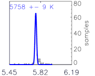
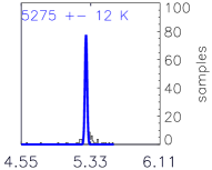
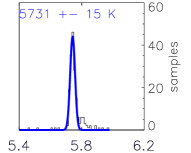
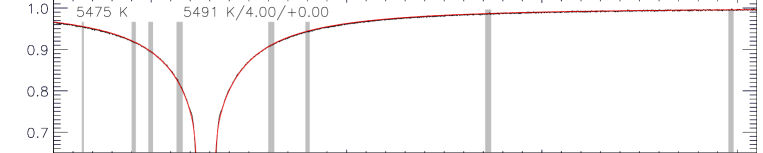
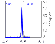
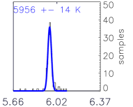
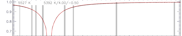
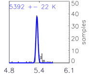
Figure 22: Fits of 3D profiles (black) with 1D profiles (red). The nominal temperature values of the 3D profiles are noted in the left, while the parameters of the 1D profiles are at the right side.

To estimate the effects of 3D models on $T_{\mathrm{eff}}$, we analyzed the synthetic H$\alpha$ profiles in the same way as the observed ones. The synthetic profiles were resampled with the same pixel size of HARPS and 0.1% of white noise was added. The fits are shown in Fig. 22 and the temperatures retrieved from 1D models are compared with their nominal temperatures in Fig. 13 as done in Sect. 6. In this figure, in the plot in function of [Fe/H], the improvement given by the 3D models (continuous red line) can be estimated by how similar the trend of Fig. 8 (dotted line here) is reproduced. The comparison show that temperatures from 1D models are practically reproduced by 3D models at [Fe/H] = 0 dex, but at [Fe/H] = $-0.5$ dex 3D models produce 100-200 hotter temperatures depending on log g. Hence, temperatures from 3D models are significantly closer to those from interferometry at [Fe/H] = $-0.5$ dex, they particularly agree for low log g values.

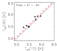
Figure 13: Same as in Fig. 8 for 3D models. In the panel on the right different symbols and colors are used for the two log g values according to the legends. The accuracy of 1D models $T_{\mathrm{eff}}=T_{\mathrm{eff}}^{H\alpha}$ $-159$[Fe/H] + 28 found in Sect. 6 is represented by the dotted line.

We therefore conclude that the most likely cause for the trend with metallicity of our H$\alpha$ diagnostics with respect to interferometric and IRFM measurements is the use of 1D models. We consider, on the other hand, and excellent approximation the use of 1D models, which are easily available, together with the correction for metallicity given in section 6.2.

10 Suitability of HARPS

Table 3: Solar proxies. The list is ordered by date of observation along with the S/N of the spectra and the effective temperature derived from H$\alpha$ profiles.

Date	object	S/N	$T_{\mathrm{eff}}^{\mathrm{H}\alpha}$ (K)
coudé
2014/10	Moon	300	$5741\pm 32$
2017/07	Moon	400	$5748\pm 25$
2017/07	Moon	400	$5746\pm 28$
2017/07	Moon	400	$5751\pm 25$
2017/07	Calisto	350	$5740\pm 28$
2017/07	Ganymede	350	$5732\pm 35$
MUSICOS
2017/11	Ganymede	300	$5726\pm 28$
2017/11	Moon	250	$5756\pm 45$
2017/11	Moon	250	$5759\pm 41$
2017/11	Moon	250	$5753\pm 30$
HARPS
2007/04	Ganymede	174	$5746\pm 52$
2007/04	Ganymede	172	$5750\pm 76$
2007/04	Ganymede	171	$5745\pm 88$
2007/04	Ganymede	173	$5745\pm 68$
2007/04	Ganymede	174	$5735\pm 99$
2007/04	Ganymede	391	$5747\pm 54$
2009/03	Moon	532	$5747\pm 32$
2010/10	Moon	263	$5741\pm 65$
2010/10	Moon	307	$5759\pm 43$
2010/10	Moon	288	$5755\pm 53$
2010/10	Moon	299	$5743\pm 74$
2010/10	Moon	308	$5753\pm 60$
2010/10	Moon	304	$5759\pm 66$
2010/12	Moon	578	$5746\pm 29$
2010/12	Moon	408	$5735\pm 38$
2010/12	Moon	412	$5744\pm 38$
2010/12	Moon	494	$5732\pm 36$
2012/06	Moon	479	$5742\pm 45$
2012/06	Moon	478	$5737\pm 48$
2012/06	Moon	488	$5746\pm 38$
2012/06	Moon	487	$5742\pm 43$
2012/06	Moon	485	$5735\pm 44$
2012/06	Moon	486	$5735\pm 42$
2012/06	Moon	488	$5739\pm 39$
2012/06	Moon	490	$5742\pm 33$
2012/06	Moon	478	$5734\pm 33$
2012/06	Moon	476	$5753\pm 35$
2014/02	Ganymede	119	$5765\pm 98$
2014/02	Ganymede	107	$5750\pm 103$
2014/02	Ganymede	117	$5760\pm 105$
2014/02	Ganymede	118	$5750\pm 107$
2014/02	Ganymede	109	$5767\pm 97$
2014/02	Ganymede	117	$5757\pm 108$
2014/02	Ganymede	116	$5744\pm 139$
2014/02	Ganymede	109	$5757\pm 138$
2014/02	Ganymede	109	$5759\pm 118$
2014/02	Ganymede	122	$5760\pm 98$
2015/07	Ceres	89	$5754\pm 134$
2015/07	Ceres	87	$5748\pm 140$
2015/07	Ceres	88	$5751\pm 111$
2015/07	Ceres	89	$5745\pm 145$
2015/07	Ceres	91	$5755\pm 137$
2015/07	Ceres	103	$5753\pm 143$
2015/07	Ceres	87	$5751\pm 126$
2015/07	Ceres	100	$5753\pm 110$
2015/07	Ceres	115	$5754\pm 116$
2015/07	Ceres	128	$5746\pm 92$

Having shown the suitability of the method with the coudé spectra, we apply it to HARPS (Mayor et al. 2003). HARPS has been chosen because, in order to achieve high radial velocity precision, the instrument has a very stable field and pupil injection. It is also thermally stable and in vacuum. In addition, HARPS archive contains a lot of observations of solar type stars, including a rich set of solar spectra taken by observing solar system bodies for many years. All these characteristics make of HARPS the ideal instrument to investigate the precision of the H$\alpha$ method we have developed. The fact that the solar siblings observations have been repeated for several years, allows us to also investigate the stability of this instrument in time, and to determine to which extent the HARPS H$\alpha$ profile has remained constant in time. The test is performed with all solar spectra set out in Table 3, for which $T_{\mathrm{eff}}^{\mathrm{H}\alpha}$’s were derived. The plot in the top panel of Fig. 14 visually summarizes the results displayed in the table. For each date, $T_{\mathrm{eff}}^{\mathrm{H}\alpha}$ values are represented by plus symbols. Their weighted mean and corresponding spread values are drawn with bars. Next to them, the number of spectra used and their average S/N ratio are noted to show the precision reached when measurements from several spectra are combined. The weighted mean and spread of all measurements are represented by the horizontal line and the shade at $5744\pm 10$ K. Evidently, there is no trend with time and the scatter is very low, which confirms the blaze stability of HARPS. This value is in perfect agreement with that of coudé (see values in Table 2), which implies that not only the blaze is stable but it is also fully removed through the flat-field procedure.

In the bottom panel of Fig. 14 we plot the precision obtained from individual spectra in function of S/N. It is observed that $\sim\!\!\!40$ K can be obtained from spectra of S/N = 400-500.

Finally, we compare the temperatures derived from HARPS with those derived from coudé spectra for the other stars in common. The comparison is shown in Fig. 15 against the three main stellar parameters. It shows an excellent agreement with a negligible offset between the two samples of $-13\pm 34$ K with no trends. The temperatures of all stars agree within 1$\sigma$ errors, with the exception of two ($\delta$ Eri and HD 184985) that agree within 2$\sigma$.

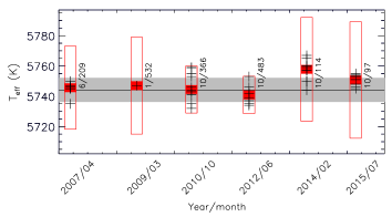
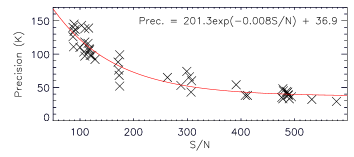
Figure 14: Top panel: Temperatures of the HARPS solar proxies in Table 3 plotted versus date. Daily values are represented by plus symbols and weighted means and errors for each month are drown in red. The weighted mean and error of all the measurements are represented by the continuous line and the shade on 5744 $\pm 10$ K. Next to the bars, the number of spectra analyzed and the mean S/N are noted. Bottom panel: The errors of individual measurements in the top panel are plotted versus S/N. The exponential curve given by the equation in the plot is the best fit to the points.

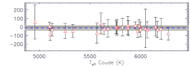
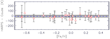
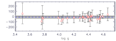
Figure 15: Temperature diagnostics from HARPS respect those of coudé vs. atmospheric parameters. [Fe/H] and log g values from Table 1 were used here. The $-13$ K offset and its 34 K scatter are represented by the dashed lines and the shades, respectively.

11 Summary and conclusions

With the aim of better understanding and minimizing the errors that affect H$\alpha$ measurements of effective temperature, we have developed a new method to analyze the spectra and tested it extensively. The results are quite consistent, and they allow us also to test the accuracy of the temperature diagnostics with H$\alpha$ profiles from 1D model atmospheres in LTE conditions (Barklem et al. 2002).

The core of this work is the special effort adopted in recovering realistic H$\alpha$ profiles free from instrumental signatures. Namely, the blaze function of the echelle spectrographs and those induced by random errors of normalization. We eliminated the blaze by using the single-order coudé instrument at do Pico dos Dias Observatory. With it, spectra of 44 F, G, and K stars, including the Sun, with a wide parameter range $T_{\mathrm{eff}}$–[Fe/H]–log g (see Fig. 1) were acquired. We minimized the errors of normalization of H$\alpha$ profiles, by integrating normalization and fit into an iterative procedure, with which we derive precise $T_{\mathrm{eff}}^{\mathrm{H}\alpha}$’s. This procedure, additionally uses synthetic spectra of telluric features of PWV to optimize the continuum location. PWV features may be very small and nearly omnipresent around H$\alpha$, so they can be easily confused with spectral noise and shift the continuum to lower flux values.

The accuracy of H$\alpha$ lines from 1D model atmospheres is found to follow the relation $T_{\mathrm{eff}}=T_{\mathrm{eff}}^{H\alpha}$ $-159$[Fe/H] + 28 within the metallicity range $-0.7$ to $+0.45$ dex. It was determined at solar parameters by $T_{\mathrm{eff}}^{\mathrm{H}\alpha}$’s from 57 coudé/HARPS/MUSICOS solar spectra (Table 3) compared with the reference solar $T_{\mathrm{eff}}$ = 5772 K (Prša et al. 2016; Heiter et al. 2015), and at non solar parameters comparing $T_{\mathrm{eff}}^{\mathrm{H}\alpha}$’s of 10 Gaia Benchmark Stars (Heiter et al. 2015) with their $T_{\mathrm{eff}}$’s from interferometric measurements.

The consistency of our results with effective temperature scales from IRFM and excitation and ionization equilibrium of Fe lines was also investigated. The comparison with IRFM using the photometric calibrations of Casagrande et al. (2010) show exactly the same trend as the interferometric one of Heiter et al. (2015) (compare Fig. 9 with Fig. 8), asserting the equivalence of the two scales. As far spectroscopic measurements, the results vary slightly with the authors, but in general they show agreement with H$\alpha$ up to 5700 K. A trend with metallicity is present and is opposite to that observed with interferometry and IRFM. Implying that the spectroscopic scale, in general, underestimates/overestimates $T_{\mathrm{eff}}$ by 100 K at [Fe/H] = $-0.6/$+0.4 dex with respect to interferometry and IRFM (see Fig. 10).

In order to investigate the observed trend with metallicity when comparing our measurements with the interferometric and IRFM ones, we tested 3D model atmospheres. H$\alpha$ profiles from 3D models produce quite similar diagnostics to 1D models at solar parameters (we obtain a $-15$ K zero point), while at the metal-poor range [Fe/H] = $-0.5$ dex, they almost fully correct 1D models underestimates (see Fig. 13). This therefore indicates that the trend with metallicity is largely due to the use of 1D models. The correction we provide by the equation above, however, brings the three scales H$\alpha$(1D + LTE), interferometry and IRFM on the same base.

We further find that the systematic “cool” solar temperature determinations from H$\alpha$ models in the literature are associated to normalization errors of the different versions of Kitt Peak National Observatory solar atlases. We quantified the impact of the errors in $T_{\mathrm{eff}}$ and find that models enhanced by 3D atmosphere geometry and NLTE conditions do improve the accuracy of 1D + LTE models, leading to practically null differences with the solar $T_{\mathrm{eff}}$ derived by Stefan-Boltzmann equation 5772 K.

We tested the suitability of HARPS for the temperature determination with H$\alpha$ profiles. The tests were performed analyzing spectra of 26 stars in common with the coudé sample and 47 solar spectra from the period 2007-2015, The solar spectra show consistent results, to better than $\pm$ 10 K, demonstrating the stability of the HARPS blaze and the goodness of the de-blazing process. The very small ($-13$ K) offset resulting from the comparison of the stars in common with the coudé sample, confirms that the normalization-fitting integrated method minimizes random normalization errors. Hence, when this method is applied, the internal errors of the H$\alpha$ profiles fitting are entirely due to the spectral noise.

Finally, in Table 4 we list $T_{\mathrm{eff}}^{\mathrm{H}\alpha}$ as measured (by combining all measurements from coudé, HARPS, and MUSICOS spectra) and our best $T_{\mathrm{eff}}$ estimate obtained applying the correction for metallicity. The [Fe/H] and log g values used for deriving $T_{\mathrm{eff}}^{H\alpha}$ follow the hierarchy Heiter15, Ramirez13, Ramirez14b, Ramirez14a, Maldonado15, Ghezzi10, Sousa08, Tsantaki13, Bensby14.

Table 4: $T_{\mathrm{eff}}$ of the sample stars. Column 4 lists the [Fe/H] values used to derive $T_{\mathrm{eff}}^{H\alpha}$ and their sources are shown in last column in the same way as in Table 1: (1) Sousa et al. (2008), (2) Ghezzi et al. (2010), (3) Tsantaki et al. (2013), (4) Ramírez et al. (2013), (5) Bensby et al. (2014), (6) Ramírez et al. (2014a), (7) Ramírez et al. (2014b), (8) Maldonado et al. (2015), (9) Heiter et al. (2015). Column 5 lists the weighted mean of the temperatures derived with coudé, HARPS, and MUSICOS spectra. Column 6 lists $T_{\mathrm{eff}}$ corrected from the H$\alpha$ diagnostics following the relation $T_{\mathrm{eff}}=T_{\mathrm{eff}}^{H\alpha}-159$[Fe/H] + 28. The errors presented are internal and are associated to the dispersion of the fit. These are the best estimates.

Name	HD	HIP	[Fe/H]	$T_{\mathrm{eff}}^{H\alpha}$ (K)	best $T_{\mathrm{eff}}$ (K)	ctlg
$\zeta$ Tuc	1581	1599	$-0.22$	$5866$	$5930\pm 17$	4
$\beta$ Hyi	2151	2021	$-0.04$	$5813$	$5848\pm 20$	9
	3823	3170	$-0.34$	$5947$	$6030\pm 18$	8
$\tau$ Cet	10700	8102	$-0.49$	$5311$	$5417\pm 22$	9
$\epsilon$ For	18907	14086	$-0.60$	$4984$	$5108\pm 48$	9
$\alpha$ For	20010	14879	$-0.30$	$6112$	$6188\pm 23$	4
$\kappa$ Cet	20630	15457	$\leavevmode\nobreak\ \leavevmode\nobreak\ \leavevmode\nobreak\ 0.00$	$5675$	$5704\pm 22$	4
$10$ Tau	22484	16852	$-0.09$	$5947$	$5990\pm 25$	4
$\delta$ Eri	23249	17378	$+0.06$	$5090$	$5110\pm 12$	9
40 Eri	26965	19849	$-0.28$	$5109$	$5182\pm 33$	4
	100623	56452	$-0.37$	$5101$	$5188\pm 17$	4
$\beta$ Vir	102870	57757	$+0.24$	$6096$	$6087\pm 18$	9
	114174	64150	$+0.05$	$5703$	$5724\pm 32$	4
$59$ Vir	115383	64792	$+0.11$	$5975$	$5987\pm 23$	4
$61$ Vir	115617	64924	$-0.02$	$5557$	$5589\pm 18$	4
$\eta$ Boo	121370	67927	$+0.32$	$6042$	$6020\pm 25$	9
	126053	70319	$-0.36$	$5663$	$5749\pm 58$	4
$\alpha$ Cen A	128620	71683	$+0.26$	$5765$	$5753\pm 12$	9
$\psi$ Ser	140538	77052	$+0.12$	$5653$	$5663\pm 21$	8
	144585	78955	$+0.29$	$5816$	$5799\pm 27$	6
18 Sco	146233	79672	$+0.06$	$5760$	$5780\pm 20$	9
	147513	80337	$+0.03$	$5805$	$5829\pm 24$	4
$\zeta$ TrA	147584	80686	$-0.08$	$6012$	$6054\pm 17$	4
12 Oph	149661	81300	$+0.01$	$5209$	$5236\pm 34$	4
	150177	81580	$-0.66$	$6056$	$6189\pm 60$	5
	154417	83601	$-0.03$	$5950$	$5984\pm 12$	4
$\mu$ Ara	160691	86796	$+0.35$	$5690$	$5664\pm 13$	9
70 Oph	165341	88601	$+0.07$	$5305$	$5323\pm 33$	4
$\iota$ Pav	165499	89042	$-0.13$	$5891$	$5941\pm 32$	8
	172051	91438	$-0.24$	$5565$	$5632\pm 71$	4
	179949	94645	$+0.2$	$6134$	$6131\pm 32$	6
31 Aql	182572	95447	$+0.41$	$5581$	$5545\pm 14$	5
	184985	96536	$+0.01$	$6255$	$6282\pm 21$	2
$\delta$ Pav	190248	99240	$+0.33$	$5633$	$5610\pm 14$	4
15 Sge	190406	98819	$+0.05$	$5904$	$5925\pm 16$	4
$\phi^{2}$ Pav	196378	101983	$-0.44$	$5979$	$6078\pm 28$	8
$\gamma$ Pav	203608	105858	$-0.66$	$5991$	$6124\pm 31$	4
	206860	107350	$-0.06$	$5878$	$5916\pm 27$	4
$\xi$ Peg	215648	112447	$-0.27$	$6125$	$6197\pm 21$	2
49 Peg	216385	112935	$-0.22$	$6193$	$6257\pm 35$	4
51 Peg	217014	113357	$+0.19$	$5785$	$5784\pm 15$	4
$\iota$ Psc	222368	116771	$-0.12$	$6150$	$6198\pm 25$	4

Appendix A H$\alpha$ profile fits