figureb
On the Transferability of Representations in Neural Networks Between Datasets and Tasks
Abstract
Deep networks, composed of multiple layers of hierarchical distributed representations, tend to learn low-level features in initial layers and transition to high-level features towards final layers. Paradigms such as transfer learning, multi-task learning, and continual learning leverage this notion of generic hierarchical distributed representations to share knowledge across datasets and tasks. Herein, we study the layer-wise transferability of representations in deep networks across a few datasets and tasks and note some interesting empirical observations.
1 Introduction
Deep networks, composed of multiple layers of hierarchical distributed representations, tend to learn low-level features in initial layers and transition to high-level features towards final layers (Zeiler and Fergus, 2014). Similar low-level features commonly appear across various datasets and tasks, while high-level features are somewhat more attuned to the dataset or task at hand, which makes low-level features more generic and easier to transfer from one dataset or task to another (Yosinski et al., 2014).
Paradigms such as transfer learning (Pan and Yang, 2010; Bengio, 2012), multi-task learning (Caruana, 1997; Misra et al., 2016), and continual learning (Li and Hoiem, 2016; Rusu et al., 2016) leverage this notion of generic hierarchical distributed representations to share knowledge across datasets and tasks. For example, in transfer learning, typically when data in the target task is scarce, the transfer of low-level features from one dataset or task to another, followed by learning high-level features, is likely to lead to a boost in performance given that both datasets or tasks share some similarity (Razavian et al., 2014). Conversely, transferring high-level features and learning low-level ones can be regarded as a form of domain adaptation and can be useful when the tasks are similar or identical but the data distributions are slightly different (Glorot et al., 2011; Bengio, 2012).
Herein, we study the layer-wise transferability of representations in deep networks across a few datasets and tasks and note some interesting empirical observations. First, the layer-wise transferability between two datasets or tasks can be non-symmetric, i.e., features learned for a primary dataset or task can be more relevant to a secondary dataset or task compared with the relevance of features learned for the secondary dataset or task to the primary one, despite both datasets being of similar size. Second, the nature of the datasets or tasks involved and their relationship is more influential on the layer-wise transferability of representations compared with other factors such as the architecture of the neural network. Third, the layer-wise transferability of representations can be used as a proxy for quantifying task relatedness. These observations highlight the importance of curriculum methods and structured approaches to designing systems for multiple tasks in the above mentioned paradigms that can maximize the knowledge transfer and minimize the interference between datasets or tasks.
Layer-wise transferability of representations in deep networks was studied in several prior studies, e.g., (Yosinski et al., 2014; Fayek et al., 2016; Misra et al., 2016). In (Yosinski et al., 2014), the transferability of learned features in a Convolutional Neural Network (ConvNet) trained for an image recognition task was experimentally studied, where the specificity versus generality of each layer in the ConvNet was quantified using curated classes from the ImageNet dataset. It was shown that initial layers in deep networks were more transferable than final layers. A similar study was carried out in (Misra et al., 2016) reporting similar findings. This work differs from the studies in (Yosinski et al., 2014; Fayek et al., 2016; Misra et al., 2016) in that we study the layer-wise transferability between more than just two image recognition datasets, i.e., CIFAR-10, CIFAR-100 (Krizhevsky, 2009), and SVHN (Netzer et al., 2011), and moreover, we study the layer-wise transferability between two speech recognition tasks, i.e., Automatic Speech Recognition (ASR) using the TIMIT dataset (Garofolo et al., 1993) and Speech Emotion Recognition (SER) using the IEMOCAP dataset (Busso et al., 2008), using more than a single ConvNet architecture, which can provide insights into the influence of neural network architectures on the transferability of representations.
2 Gradual Transfer Learning
The methodology for quantifying the layer-wise transferability of representations between two datasets or tasks, denoted gradual transfer learning, is as follows. First, two primary neural network models that comprise layers are trained for each dataset or task independently. Second, for each of the two primary models, the learned parameters in all layers of the trained model, except the output layer, are copied to a new model for the (other) secondary dataset or task; the output layer can be randomly initialized, since it is closely tied to the dataset or task at hand, e.g., the number of output classes in both datasets or tasks may be different. Third, the first layers are held constant and the remaining layers are fine-tuned for the secondary dataset or task, where is the number of hidden layers in the model, i.e., . If the constant transferred layers are relevant to the secondary dataset or task, one can expect an insignificant or no drop in performance relative to the primary model trained independently, and vice versa. By iteratively varying the number of constant layers , the layer-wise transferability of representations learned for each dataset or task to the other can be inferred.
Iterating through yields a number of special cases as follows. In the case of , the primary model can be regarded as a feature extractor to the secondary model, in that the output layer is the only layer to be fine-tuned. In the case of , the output layer is first fine-tuned for a small number of iterations to avoid back-propagating gradients from randomly initialized parameters to previous layers when the output layer is randomly initialized, and subsequently the final layers (including the output layer) are fine-tuned simultaneously. In the case of , the output layer is first fine-tuned for a small number of iterations, and then all layers of the model are fine-tuned simultaneously with the output layer; in this case, the primary model can be regarded as only an initialization to the secondary model.
3 Experiments and Results
Layer-wise transferability between the CIFAR-10, CIFAR-100, and SVHN datasets.
The CIFAR-10, CIFAR-100, and SVHN datasets are chosen to study how task relatedness can influence the layer-wise transferability. The CIFAR-10 and CIFAR-100 datasets are both natural images labelled into and classes respectively, whereas, the SVHN dataset is street view images of house numbers labelled into classes corresponding to the digits; i.e., it can be expected that the CIFAR-10 and CIFAR-100 datasets are more closely related to each other compared with the SVHN dataset. For each CIFAR dataset, the original training set was split into a training set of images and a validation set of images; the entire test set was used for testing. For the SVHN dataset, the original training set and additional set were combined and split into a training set of images and a validation set of images; the entire test set was used for testing. Standard dataset pre-preprocessing was applied to all datasets (Goodfellow et al., 2013; Long et al., 2015), i.e., the mean and standard deviation of the images in the CIFAR datasets were normalized to zero and one respectively using the mean and standard deviation computed from the training set, while, the images in the SVHN dataset were divided by to lie in the range.
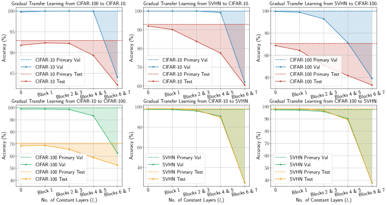
The model used in this experiment follows the Densely Connected Convolutional Networks (DenseNet) architecture (Huang et al., 2017) that comprises layers (see supplementary material for more details). It was shown to achieve state-of-the-art performance on the datasets used in this experiment (Huang et al., 2017). The main layers in the architecture can be grouped into blocks based on their type and role. The first block, Block , is a standard convolutional layer. The dense blocks, Blocks , , and , comprise layers of Batch Normalization (BatchNorm), Rectified Linear Units (ReLUs), convolution, and dropout. Each convolution layer in Blocks , , and is connected to all subsequent layers in the same block via the concatenation operation. The transition blocks, Blocks and , are used to counteract the growth in the number of parameters due to the use of the concatenation operation, and are composed of a layer of BatchNorm, ReLUs, convolution, dropout, and average pooling. A down-sampling block, Block , is used to further reduce the complexity of the model, and is composed of BatchNorm, ReLUs, and average pooling. The output layer is a fully connected layer followed by a softmax function. The models were trained following the settings detailed in (Huang et al., 2017). Three primary models were trained independently for the CIFAR-10, CIFAR-100, and SVHN datasets. Gradual transfer learning was used to assess the layer-wise transferability of the learned representations for each dataset to the other two. Due to the large number of layers in the model, the number of fixed layers was varied in block intervals as opposed to single layer intervals, i.e., .
The results of gradual transfer learning between the CIFAR-10, CIFAR-100, and SVHN datasets are plotted in Figure 1. It is observed that the representations learned in the CIFAR-10 and CIFAR-100 datasets are more transferable, i.e., lead to a smaller degradation in performance compared with the primary model, to all other datasets compared with the representations learned in the SVHN dataset. The learned representations in the SVHN dataset were less transferable to the CIFAR-10 and CIFAR-100 datasets suggesting that the layer-wise transferability of learned representations can be non-symmetric, and moreover, dependant on the nature of the primary and secondary datasets or tasks. Note that the classes in the CIFAR datasets are more general than the classes in the SVHN dataset that correspond to digits to .
Layer-wise transferability between the TIMIT and IEMOCAP datasets.
Both tasks, the ASR task and the SER task, are speech recognition tasks, yet the relatedness between both tasks is somewhat fuzzy (see (Fayek et al., 2016) for more details). For the TIMIT dataset, the complete -speaker training set, without the dialect (SA) utterances, was used as the training set; the -speaker development set was used as the validation set; the -speaker core test set was used as the test set. For the IEMOCAP dataset, utterances that bore only the following four emotions: anger, happiness, sadness, and neutral, were used, with excitement considered as happiness, amounting to a total of utterances. An eight-fold leave-one-speaker-out cross-validation scheme was employed in all experiments using eight speakers, while the remaining two speakers were used as a validation set. The results in this experiment are the average of the eight-fold cross-validation. For both datasets, utterances were split into frames with a stride of , and a Hamming window was applied, then -MFSCs were extracted from each frame. The mean and standard deviation were normalized per coefficient to zero and one respectively using the mean and standard deviation computed from the training set only in the case of ASR and from training subset in each fold in the case of SER.
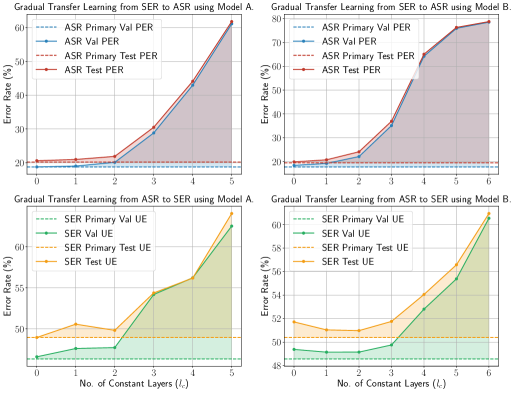
The ASR system had a hybrid ConvNet-HMM architecture. A ConvNet acoustic model was used to produce a probability distribution over the states of three-state HMMs with a bi-gram language model estimated from the training set. The SER system comprised only a ConvNet acoustic model identical to the model used in ASR. Two ConvNet architectures were used to isolate architecture-specific behaviour and trends. The first architecture, denoted Model A, is a standard ConvNet that comprises two convolutional and max pooling layers, followed by four fully connected layers, with BatchNorm and ReLUs interspersed in-between (see supplementary material for more details). The second architecture, denoted Model B, is a variant of the popular VGGNet architecture (Sercu et al., 2016). The architecture comprises a number of convolutional, BatchNorm, and ReLUs layers, with a few max pooling layers used throughout the architecture (see supplementary material for more details), followed by three fully connected layers, with BatchNorm, ReLUs, and dropout interspersed in-between. In both architectures, the final fully connected layer is followed by a softmax function to predict the probability distribution over classes in the case of ASR, i.e., three HMM states per phonemes, or classes in the case of SER. The models were trained following the settings detailed in (Fayek et al., 2016). Two primary models were trained independently for the TIMIT and IEMOCAP datasets for each architecture. Gradual transfer learning was used to assess the layer-wise transferability of the learned representations for each dataset to the other one.
The results of gradual transfer learning between the TIMIT and IEMOCAP datasets are plotted in Figure 2. It is observed that both architectures exhibit similar behaviour, where initial layers are more transferable than final layers and the transferability decreases gradually as we traverse deeper into the network. With the exception of a few outliers, the layer-wise transferability was similar for both architectures, despite the differences between both architectures in the number and type of layers.
4 Discussion
The layer-wise transferability of representations was explored on a variety of neural network architectures, datasets, and tasks. As demonstrated in Figure 1, the layer-wise transferability between two datasets or tasks can be non-symmetric, where the representations learned in the CIFAR-10 and CIFAR-100 datasets were found to be more transferable than the representations learned in the SVHN dataset. This reflects the nature of the classes in the CIFAR datasets, which are more general, compared with the classes in the SVHN dataset, which correspond to digits to . As demonstrated in Figure 2, the nature of the datasets or tasks involved and their relationship is more influential on the transferability of representations compared with the architecture of the neural network. Generally, consistent behaviour emerged reflecting the nature of the datasets or tasks involved. These observations highlight the importance of curriculum methods and structured approaches to designing systems for multiple tasks in paradigms that incorporate learning multiple tasks to maximize the knowledge transfer and minimize the interference between datasets or tasks.
Acknowledgments
H. M. Fayek is funded by the Vice-Chancellor’s Ph.D. Scholarship (VCPS) from RMIT University. This research was undertaken with the assistance of resources and services from the National Computational Infrastructure (NCI), which is supported by the Australian Government. The authors gratefully acknowledge the support of NVIDIA Corporation with the donation of one of the Tesla K40 GPUs used for this research.
References
- Bengio [2012] Yoshua Bengio. Deep learning of representations for unsupervised and transfer learning. In International Conference on Machine Learning (ICML) Workshop on Unsupervised and Transfer Learning, pages 17–36, 2012.
- Busso et al. [2008] C. Busso, M. Bulut, C.-C. Lee, A. Kazemzadeh, E. Mower, S. Kim, J.N. Chang, S. Lee, and S.S. Narayanan. IEMOCAP: interactive emotional dyadic motion capture database. Language Resources and Evaluation, 42(4):335–359, 2008. ISSN 1574-020X.
- Caruana [1997] Rich Caruana. Multitask learning. Machine Learning, 28(1):41–75, July 1997. ISSN 0885-6125.
- Fayek et al. [2016] Haytham M. Fayek, Margaret Lech, and Lawrence Cavedon. On the correlation and transferability of features between automatic speech recognition and speech emotion recognition. In Interspeech, pages 3618–3622, 2016. doi: 10.21437/Interspeech.2016-868.
- Garofolo et al. [1993] John S Garofolo, Lori F Lamel, William M Fisher, Jonathan G Fiscus, David S Pallett, N. Dahlgren, and V. Zue. Timit acoustic-phonetic continuous speech corpus. Linguistic Data Consortium, 93, 1993.
- Glorot et al. [2011] Xavier Glorot, Antoine Bordes, and Yoshua Bengio. Domain adaptation for large-scale sentiment classification: A deep learning approach. In International Conference on Machine Learning (ICML), pages 513–520, 2011.
- Goodfellow et al. [2013] Ian Goodfellow, David Warde-Farley, Mehdi Mirza, Aaron Courville, and Yoshua Bengio. Maxout networks. In International Conference on Machine Learning (ICML), volume 28, pages 1319–1327, Atlanta, Georgia, USA, June 2013. URL http://proceedings.mlr.press/v28/goodfellow13.html.
- Huang et al. [2017] Gao Huang, Zhuang Liu, Kilian Q Weinberger, and Laurens van der Maaten. Densely connected convolutional networks. In IEEE Conference on Computer Vision and Pattern Recognition (CVPR), 2017.
- Krizhevsky [2009] Alex Krizhevsky. Learning multiple layers of features from tiny images. Technical report, University of Toronto, 2009.
- Li and Hoiem [2016] Zhizhong Li and Derek Hoiem. Learning without forgetting. In European Conference on Computer Vision (ECCV), pages 614–629. Springer, 2016. ISBN 978-3-319-46493-0. doi: 10.1007/978-3-319-46493-0_37.
- Long et al. [2015] Jonathan Long, Evan Shelhamer, and Trevor Darrell. Fully convolutional networks for semantic segmentation. In IEEE Conference on Computer Vision and Pattern Recognition (CVPR), pages 3431–3440, 2015.
- Misra et al. [2016] Ishan Misra, Abhinav Shrivastava, Abhinav Gupta, and Martial Hebert. Cross-stitch networks for multi-task learning. In IEEE Conference on Computer Vision and Pattern Recognition (CVPR), pages 3994–4003, 2016.
- Netzer et al. [2011] Yuval Netzer, Tao Wang, Adam Coates, Alessandro Bissacco, Bo Wu, and Andrew Y Ng. Reading digits in natural images with unsupervised feature learning. In Advances in Neural Information Processing Systems (NIPS) workshop on deep learning and unsupervised feature learning, 2011.
- Pan and Yang [2010] Sinno Jialin Pan and Qiang Yang. A survey on transfer learning. IEEE Transactions on Knowledge and Data Engineering, 22(10):1345–1359, 2010.
- Razavian et al. [2014] A. S. Razavian, H. Azizpour, J. Sullivan, and S. Carlsson. CNN features off-the-shelf: An astounding baseline for recognition. In IEEE Conference on Computer Vision and Pattern Recognition (CVPR) Workshops, pages 512–519, June 2014. doi: 10.1109/CVPRW.2014.131.
- Rusu et al. [2016] Andrei A. Rusu, Neil C. Rabinowitz, Guillaume Desjardins, Hubert Soyer, James Kirkpatrick, Koray Kavukcuoglu, Razvan Pascanu, and Raia Hadsell. Progressive neural networks. CoRR, abs/1606.04671, 2016.
- Sercu et al. [2016] Tom Sercu, Christian Puhrsch, Brian Kingsbury, and Yann LeCun. Very deep multilingual convolutional neural networks for lvcsr. In IEEE International Conference on Acoustics, Speech and Signal Processing (ICASSP), pages 4955–4959. IEEE, 2016.
- Yosinski et al. [2014] Jason Yosinski, Jeff Clune, Yoshua Bengio, and Hod Lipson. How transferable are features in deep neural networks? In Advances in Neural Information Processing Systems (NIPS), pages 3320–3328. Curran Associates, Inc., 2014.
- Zeiler and Fergus [2014] Matthew D. Zeiler and Rob Fergus. Visualizing and understanding convolutional networks. In European Conference on Computer Vision (ECCV), pages 818–833, Cham, 2014. Springer. ISBN 978-3-319-10590-1.
Supplementary Material
Table 1 details the ConvNet architecture used in the image recognition experiment. Table 1 and Table 1 detail respectively the ConvNet architecture for Model A and Model B used in the speech recognition experiment.
| Block | Repeat | Type | Size | Other |
|---|---|---|---|---|
| 1 | Convolution | Stride = 1 | ||
| 2 | BatchNorm | — | — | |
| ReLU | — | — | ||
| Convolution | Stride = 1 | |||
| Dropout | — | |||
| 3 | BatchNorm | — | — | |
| ReLU | — | — | ||
| Convolution | Stride = 1 | |||
| Dropout | — | |||
| Average Pooling | Stride = 2 | |||
| 4 | BatchNorm | — | — | |
| ReLU | — | — | ||
| Convolution | Stride = 1 | |||
| Dropout | — | |||
| 5 | BatchNorm | — | — | |
| ReLU | — | — | ||
| Convolution | Stride = 1 | |||
| Dropout | — | |||
| Average Pooling | Stride = 2 | |||
| 6 | BatchNorm | — | — | |
| ReLU | — | — | ||
| Convolution | Stride = 1 | |||
| Dropout | — | |||
| 7 | BatchNorm | — | — | |
| ReLU | — | — | ||
| Average Pooling | Stride = 8 | |||
| 8 | Fully Connected | — | ||
| Softmax | — | — |
| No. | Type | Size | Other |
| 1 | Convolution | Stride = 1 | |
| BatchNorm | — | — | |
| ReLU | — | — | |
| Max Pooling | Stride = 2 | ||
| 2 | Convolution | Stride = 1 | |
| BatchNorm | — | — | |
| ReLU | — | — | |
| Max Pooling | Stride = 2 | ||
| 3 | Fully Connected | — | |
| BatchNorm | — | — | |
| ReLU | — | — | |
| Dropout | — | ||
| 4 | Fully Connected | — | |
| Batch Norm | — | — | |
| ReLU | — | — | |
| Dropout | — | ||
| 5 | Fully Connected | — | |
| BatchNorm | — | — | |
| ReLU | — | — | |
| Dropout | — | ||
| 6 | Fully Connected | — | |
| Softmax | — | — |
| No. | Repeat | Type | Size | Other |
| 1 | Convolution | Stride = 1 | ||
| BatchNorm | — | — | ||
| ReLU | — | — | ||
| Convolution | Stride = 1 | |||
| BatchNorm | — | — | ||
| ReLU | — | — | ||
| Max Pooling | Stride = 2 | |||
| 2 | Convolution | Stride = 1 | ||
| BatchNorm | — | — | ||
| ReLU | — | — | ||
| Max Pooling | Stride = 2 | |||
| 3 | Convolution | Stride = 1 | ||
| BatchNorm | — | — | ||
| ReLU | — | — | ||
| Max Pooling | Stride = 2 | |||
| 4 | Convolution | Stride = 1 | ||
| BatchNorm | — | — | ||
| ReLU | — | — | ||
| Max Pooling | Stride = 2 | |||
| 5 | Fully Connected | — | ||
| BatchNorm | — | — | ||
| ReLU | — | — | ||
| Dropout | — | |||
| 6 | Fully Connected | — | ||
| BatchNorm | — | — | ||
| ReLU | — | — | ||
| Dropout | — | |||
| 7 | Fully Connected | — | ||
| Softmax | — | — |