Large-scale Generative Modeling to Improve Automated Veterinary Disease Coding

Abstract

Supervised learning is limited both by the quantity and quality of the labeled data. In the field of medical record tagging, writing styles between hospitals vary drastically. The knowledge learned from one hospital might not transfer well to another. This problem is amplified in veterinary medicine domain because veterinary clinics rarely apply medical codes to their records. We proposed and trained the first large-scale generative modeling algorithm in automated disease coding. We demonstrate that generative modeling can learn discriminative features when additionally trained with supervised fine-tuning. We systematically ablate and evaluate the effect of generative modeling on the final system’s performance. We compare the performance of our model with several baselines in a challenging cross-hospital setting with substantial domain shift. We outperform competitive baselines by a large margin. In addition, we provide interpretation for what is learned by our model.

1 Introduction

One of the most significant challenges for veterinary data science is that veterinary primary practices rarely code clinical findings in EHR records. This makes it hard to perform core tasks like case finding, cohort selection, or to support the production of basic descriptive statistics like disease prevalence. It is becoming increasingly accepted that spontaneous diseases in animals have important translational impact on the study of human disease for a variety of disciplines (Kol et al., 2015). Beyond the study of zoonotic diseases, which represent 60-70% of all emerging diseases, non-infectious diseases, like cancer, have become increasingly studied in companion animals as a way to mitigate some of the problems with rodent models of disease (LeBlanc, Mazcko, and Khanna, 2016). Additionally, spontaneous models of disease in companion animals are being used in drug development pipelines as these models more closely resemble the “real world” clinical settings of diseases than genetically altered mouse models (Grimm, 2016; Klinck et al., 2017; Baraban and Löscher, 2014; Hernandez et al., 2018).

In comparison to the human EHR, there has been little ML work on veterinary EHR, which faces a unique challenge. The labeled data which are accessible to research only reside in referral teaching hospitals. These hospitals often specialize in a specific type of diseases. The patient type, as well as the disease distributions, do not resemble the general population. Machine learning models trained on this dataset might easily get biased and perform poorly on general clinical records. We refer to this as the cross-hospital challenge.

Our contributions

We develop an algorithm to leverage one million unlabeled clinical notes through generative sequence modeling, and demonstrate such large-scale modeling can substantially improve the model’s performance in a cross-hospital setting. We adapt the new state-of-the-art Transformer model proposed by Vaswani et al. (2017). We systematically evaluate the model performance in this cross-hospital setting, where the algorithm trained on one hospital is evaluated in a different hospital with substantial domain shift. In addition, we provide interpretation for what is learned by the deep network. Our algorithm addresses an important application in healthcare, and our experiments add insights into the power of generative sequence modeling for clinical NLP.

2 Task and Data

We formulate the problem of automated disease coding as a multi-label classification problem. Given a veterinary record $\bm{\mathrm{X}}$, which contains detailed description of the diagnosis, we try to infer a subset of diseases $\bm{y}\in\mathcal{\bm{Y}}$, given a pre-defined set of diseases $\mathcal{\bm{Y}}$. The problem of inferring a subset of disease codes can be viewed as a series of independent binary prediction problems (Sorower, 2010).

We use three datasets in this work (Appendix Table S1). CSU(Labeled): We use a curated set of 112,558 veterinary notes from the Colorado State University College of Veterinary Medicine and Biomedical Sciences. Each note is annotated with a set of SNOMED-CT codes by veterinarians at Colorado State. PP(Labeled): We obtain a smaller set of 586 discharge summaries curated from a commercial veterinary practice located in Northern California. Two veterinary experts applied SNOMED-CT codes to these records and achieved consensus on the records used for validation. This dataset is drastically different from the CSU dataset evidenced by their shorter length and usage of abbreviations. SAGE(Unlabeled): We obtained a large set of 1,019,747 unlabeled notes from the SAGE Centers for Veterinary Specialty & Emergency Care. This is a set of raw clinical notes without any codes applied to them. The characteristics of this dataset should be similar to the PP dataset because they are both primary local clinics.

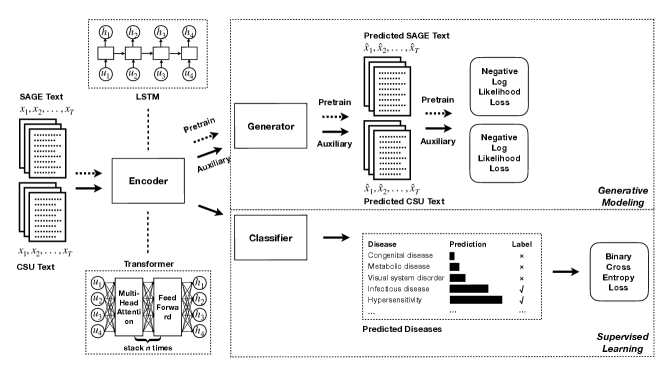
Figure 1: Our proposed model architecture for automated disease coding. Two tasks are shown: generative modeling (top) and supervised learning (bottom). The dashed arrows represent the generative modeling process on the unlabeled SAGE data, and the solid arrows represent the supervised learning process on the labeled CSU data. An additional test is done on the PP data (not shown).

	CSU				PP (Cross-hospital)
Model	EM	P	R	$F_{1}$	EM	P	R	$F_{1}$
Metamap(SVM)	32.2	74.8	75.0	74.8	3.2	57.3	53.1	51.6
Metamap(MLP)	41.2	82.6	71.8	76.4	13.8	56.4	47.6	50.5
CAML(Mullenbach et al., 2018)	46.7	86.9	76.1	80.5	16.9	72.2	50.2	54.7
LSTM	46.7	87.5	74.2	79.5	17.8	74.8	49.6	54.9
LSTM+Word2Vec	47.2	86.4	76.6	80.7	20.4	75.8	48.6	54.3
LSTM+Pretrain	48.2	87.4	76.2	81.0	20.1	73.8	52.0	57.6
LSTM+Auxiliary	49.2	88.2	76.0	81.0	20.8	75.2	53.8	58.7
LSTM+Auxiliary+Pretrain	49.0	87.6	76.5	81.2	19.6	75.5	54.8	60.3
Transformer	45.1	86.3	73.5	78.6	17.3	73.3	54.5	58.5
Transformer+Word2Vec	41.2	87.2	68.9	75.2	18.8	77.1	50.5	55.2
Transformer+Pretrain	46.6	87.5	74.6	79.6	19.9	73.5	50.5	55.4
Transformer+Auxiliary	49.4	87.3	78.5	82.2	22.2	75.0	59.3	63.6
Transformer+Auxiliary+Pretrain	50.1	88.3	77.4	81.8	25.2	75.4	64.5	68.0

Table 1: Evaluation of trained classifiers on the CSU test data and PP data. EM is the fraction of cases where the set of diseases predicted by the model exactly matches the expert labels. The classifiers are trained on a subset of CSU. Notation: LSTM and Transformer are our two base encoder models; +Word2Vec uses Word2Vec trained on SAGE to initialize; +Pretrain uses generative modeling loss $-\log p(X)$ on SAGE to initialize; +Auxiliary uses generative modeling loss on CSU in addition to classification objective on CSU: $L(\mathcal{C})-\lambda*\log p(X)$.

3 Our Model

Our proposed model architecture is shown in Figure 1. Two tasks are shown: generative modeling and supervised learning. We describe these two tasks in the following section.

3.1 Generative Modeling

A generative model over text is also referred to as a language model. Text sequence is an ordered list of tokens. Therefore, we can build an autoregressive model to estimate the joint probability of the entire sequence: $p(X)=p(x_{1},...,x_{T})$. In an ordered sequence, we can factorize it as $p(X)=\prod_{t=1}^{T}p(x_{t}|x_{1},...,x_{t-1})$. Concretely, we estimate the token distribution of $x_{t}$ by using the contextualized representation provided by our encoder: $h_{t}=\mathrm{Encoder}(h_{1},...,h_{t-1})$. We optimize over the negative log-likelihood of the distribution $-\log p(X)=-\sum_{t=1}^{T}\log p(x_{t}|x_{1},...,x_{t-1})$.

In our model, we examine the effect of generative modeling on two encoder architectures: Transformer and the Long Short-Term Memory (LSTM) (Hochreiter and Schmidhuber, 1997). We use this objective in two parts of our system: 1) pretrain encoder’s parameters; 2) serve as an auxiliary task during training of the classifier.

3.2 Supervised Learning

Classifier uses a dot-product attention layer to get a summary representation $c$ for the entire sequence. We describe the computation in Appendix Eqn 5. We then use a fully connected layer to down project it and calculate probability: $p(y_{j})=\sigma(w_{j}^{T}c+b_{j})$. We compute the binary cross entropy loss across $m$ labels: $L(\mathcal{C})=-\frac{1}{m}\sum_{j=1}^{m}y_{j}\log p(y_{j})+(1-y_{j})\log(1-p(y_{j}))$.

Finally, we use a mixture of two losses $L_{\mathrm{total}}=L(\mathcal{C})-\lambda*\log p(X)$ and use hyperparameter $\lambda=0.5$ to set the strength of the auxiliary task loss when we use generative modeling as an auxiliary task in our classification training.

Disease (SNOMED-CT code)	Extracted Keywords
Traumatic AND/OR non-traumatic injury	fracture, wound, laceration, due, assessment,
	trauma, this, bandage, time, owner
Visual system disorder	eye, ophthalmology, surgery, eyelid, assessment,
	sicca, time, uveitis, diagnosed, this
Hypersensitivity condition	dermatitis, allergic, therapy, atopic, otitis,
	pruritus, ears, assessment, allergies, dermatology
Metabolic disease	diabetes, nph, hypercalcemia, glargine, vetsulin,
	weeks, home, insulin, amlodipine, dose
Anemia	pancytopenia, anemia, visit, hemolytic, persistent,
	steroids, hypertension, neoplasia, exam, thickening

Table 2: Most influential words in the best model (Transformer+Auxiliary+Pretrain). We select five representative disease categories. For each disease, we show the top 10 words in the MetaMap medical dictionary that the model most strongly associates with the disease.

4 Results

We conduct systematic experiments on different models and ablations to quantify which component of our model improves the automatic coding performance (Table 1).

Neural networks outperform feature-based models

We use the popular MetaMap, a program developed by the National Library of Medicine (NLM) (Aronson and Lang, 2010), as a baseline. MetaMap processes a document and outputs a list of matched medically-relevant keywords with its frequencies in the given document. We directly train on the sparse bag-of-words feature representation from MetaMap. We use SVM or MLP as the classification algorithm from scikit-learn (Pedregosa et al., 2011). We find its performance is worse than the CAML, LSTM and Transformer on both the CSU and PP test data.

Generative modeling outperforms Word2Vec

The test perplexity of the generative modeling can achieve on the SAGE dataset with LSTM is 20.7 and with Transformer is 15.6. Transformer outperforms LSTM on generative modeling pretraining. We find that generative modeling as pretrain is sufficient for models to learn useful word embeddings and models with +Pretrain outperforms models with +Word2Vec on both CSU and cross-hospital dataset PP.

Generative modeling helps Transformer more

In our experiment, we compare the performance of our system by adding generative modeling objective as an auxiliary task during the classification task. Adding the generative modeling as an auxiliary task improves both Transformer and LSTM on CSU test set as well as the cross-hospital PP evaluation set. The effect of auxiliary training is more significant on Transformer than on LSTM. We also combine the generative modeling pretraining as well as the auxiliary task during the classification task and observe a substantially better performance on the overall model compared to the baseline model with either encoder.

5 Interpretation

In order to gain intuition on how deep learning models process clinical notes, we implement a gradient-based interpretation method on our model. The method attributes prediction scores to input by computing the attribution score as gradient $\times$ input (Ancona et al., 2018). We compute the frequency of words that have score $\geq 0.2$ (threshold chosen to select on average 3% words per note), use MetaMap dictionary as a filter to extract medical relevant terms, and then sort them in decreasing order. We sample 5 diseases and report the top 10 clinical relevant terms extracted by the model in the Table 2. Words captured by the model have high quality and agree with medical domain knowledge. Most words captured by the model are in the expert-curated dictionary from the MetaMap. Moreover, we notice that the model is capable of capturing abbreviations (i.e., ‘kcs’), combinations (i.e., ‘immune-mediated’) and rare professional terms (i.e., ‘cryptorchid’) that MetaMap fails to extract.

6 Conclusion

We propose a framework that is robust for the cross-hospital generalization problem in the veterinary medicine automated coding task. By training the model on 1 million raw notes with generative modeling objective, and using state-of-the-art Transformer model, we substantially increase the performance of the framework on clinical notes annotated and gathered from a private hospital. Our framework can be applied to other medical domains that currently lack medical coding resources.

Appendix A Supplementary Material

A.1 Model Details

LSTM

The Long short-term Memory Networks (LSTM) is a recurrent neural network with a long short-term memory cell (Hochreiter and Schmidhuber, 1997). It maintains semantic gating functions specifically designed to capture long-term dependency between words. At time step $t$ with word embedding input $x_{t}$, the recurrent computation of the LSTM networks can be described in Equation 1. $\sigma$ is the sigmoid function $\sigma=1/(1+e^{-x})$, and $\tanh$ is the hyperbolic tangent function. $\odot$ indicates the hadamard product.

$$\begin{split}f_{t}&=\sigma(W_{f}x_{t}+V_{f}h_{t-1}+b_{f})\\ i_{t}&=\sigma(W_{i}x_{t}+V_{i}h_{t-1}+b_{i})\\ o_{t}&=\sigma(W_{o}x_{t}+V_{o}h_{t-1}+b_{o})\\ \tilde{c}_{t}&=\tanh(W_{c}x_{t}+V_{c}h_{t-1}+b_{c})\\ c_{t}&=f_{t}\odot c_{t-1}+i_{t}\odot\tilde{c}_{t}\\ h_{t}&=o_{t}\odot\tanh(c_{t})\end{split}$$ (1)

Transformer

Transformer was proposed by Vaswani et al. (2017) as a machine translation architecture. We use a multi-layer Transformer decoder similar to the setup in  Radford et al. (2018).

Let the previous layer’s output as $H^{l-1}=[h_{1}^{l-1},h_{2}^{l-1},...,h_{T}^{l-1}]$. At the first layer, these values equal to word embeddings added with a positional encoding defined in Equation 2 where $i$ indicates the dimension of the positional embedding, and $t$ indicates the position of this token in the sequence.

For the multihead attention, we first use three linear projections to transform $H^{l-1}$ to $K^{(i)}$, $V^{(i)}$, and $Q^{(i)}$ matrices. We compute the new hidden states $H^{(i)}$ according to Equation 3.

$$\begin{split}\mathrm{PE}(t,2i)&=\sin(t/10000^{2i/d})\\ \mathrm{PE}(t,2i+1)&=\cos(t/10000^{2i/d})\end{split}$$ (2)

$$\begin{split}\left(\begin{array}[]{ll}K^{(i)}\\ Q^{(i)}\\ V^{(i)}\\ \end{array}\right)&=\left(\begin{array}[]{ll}W^{(i)}_{k}\\ W^{(i)}_{q}\\ W^{(i)}_{v}\\ \end{array}\right)H^{l-1}+\left(\begin{array}[]{ll}b^{(i)}_{k}\\ b^{(i)}_{q}\\ b^{(i)}_{v}\\ \end{array}\right)\\ \tilde{H}^{(i)}&=V^{(i)}(\mathrm{SoftMax}(\frac{Q^{(i)^{T}}K^{(i)}}{\sqrt{d}}\odot M))\\ H^{(i)}&=W^{(i)}_{h}\tilde{H}^{(i)}+b^{(i)}_{h}\\ \end{split}$$ (3)

$$\begin{split}\tilde{H}^{l}&=\mathrm{Concat}(H^{(1)},H^{(2)},...,H^{(n)})\\ H^{l}&=W_{o_{2}}\mathrm{ReLU}(W_{o_{1}}\tilde{H}^{l}+b_{o_{1}})+b_{o_{2}}\\ \end{split}$$ (4)

An n-headed attention computes Equation 3 $n$ times and concatenate the obtained $H^{(i)}\in\mathbb{R}^{T\times(d/n)}$ matrix $n$ times. In order to prevent dimension blow-up as the layer goes deeper, multi-head attention matrix $W^{(i)}_{k},W^{(i)}_{q},W^{(i)}_{v}$ all have dimensions $(d/n)\times d$. In Equation 4, we describe the transformer block. The matrix multiplication by $W_{o_{1}}\in\mathbb{R}^{D\times d},W_{o_{2}}\in\mathbb{R}^{d\times D}$ are referred to as a bottleneck computation, where $D$ is much larger than $d$.

Classifier

The drawback of letting $c=h_{T}$ is that we are essentially reducing the information before timestamp $T$. We use a dot-product attention layer to transform $\{h_{1},...,h_{T}\}$ to a vector that summarizes the entire sequence $c$. The computation is defined in Equation 5.

$$\begin{split}\tilde{h}^{(k)}_{T}&=W^{(k)}h_{T}+b^{(k)}\\ \alpha_{i}^{(k)}&=\frac{\operatorname{exp}\left(h_{i}\cdot\tilde{h}^{(k)}_{T}\right)}{\sum_{j=1}^{T}\operatorname{exp}\left(h_{j}\cdot\tilde{h}^{(k)}_{T}\right)}\\ c^{(k)}&=\sum_{j=1}^{T}\alpha_{i}^{(k)}h_{i}\\ c&=\mathrm{Concat}(c^{(1)},c^{(2)},...,c^{(n)})\\ \end{split}$$ (5)

Experimental Setup

We filter out all non-ascii characters in our documents, convert all letters to lower case, and then tokenize with NLTK (Bird and Loper, 2004). We apply the standard BPE (Byte Pair Encoding) (Sennrich, Haddow, and Birch, 2015) algorithm to address the out-of-vocabulary problem. BPE uses a vocabulary size of 50k. We truncate all documents to no more than 600 tokens, padded with start and end of sentence tokens. The word embedding dimension and encoder latent dimension are both set to 768. For the Transformer, we stack 6 transformer blocks, with 8 heads for the multi-head attention on each layer. We let the feedforward dimension to be 2048. We implement our model in PyTorch. We use Noam Optimizer (Vaswani et al., 2017) with 8000 warm up steps. Dropout rate is set to 0.1 during training to reduce overfitting. We split datasets into training, validation and test set (Table S1). All models are trained for 10 epochs. We use the validation set to select our best model and evaluate CSU test set and PP test set on our best model. We use a batch size of 10 for LSTM and a batch size of 5 for Transformer, which is the maximum allowed to train on a single GPU.

A.2 Dataset Details

	CSU	PP	SAGE
	(Labeled)	(Labeled)	(Unlabeled)
# of notes	112,557	586	1,019,747
# of training set	101,301(90%)	0(0%)	917,665(90%)
# of validation set	5,628(5%)	0(0%)	51,103(5%)
# of test set	5,628(5%)	586(100%)	50,979(5%)
Avg # of words	368	253	72
Average # of BPE tokens	374	267	73

Table S1: Descriptive statistics of the three datasets.

SNOMED-CT Codes

SNOMED-CT is a comprehensive clinical health terminology managed by the International Health Terminology Standards Development Organization (Donnelly, 2006). Annotations are applied from the SNOMED-CT veterinary extension (SNOMED-CT VET), which is a veterinary extension of the International SNOMED-CT edition. In this work, we try to predict disease level SNOMED-CT codes.

Example

We select three examples from each dataset and show them in Figure S1.

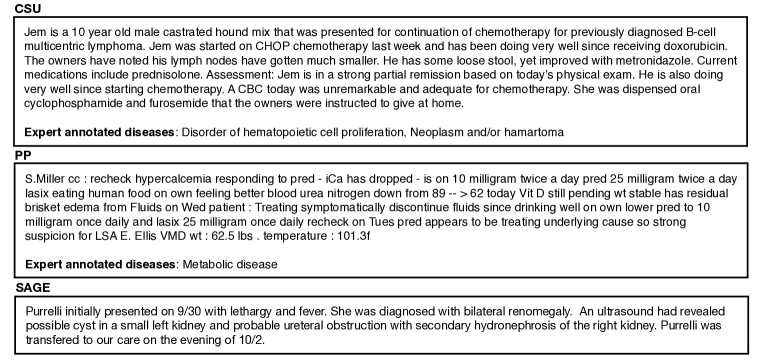
Figure S1: Examples from the CSU, PP and SAGE datasets. CSU and PP are expert labeled and SAGE is unlabeled.

Length Distribution

We plot a histogram to show the proportion of records in each dataset with certain length in Figure S3.

Number of Label Per Document Distribution

We plot a histogram to show the proportion of records in each labeled dataset with certain number of labels in Figure S3.

Species Distribution

We plot pie charts to show the proportion of species in each labeled dataset in Figure S4.

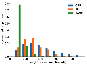
Figure S2: Document length distribution.

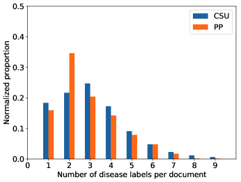
Figure S3: Label number distribution.

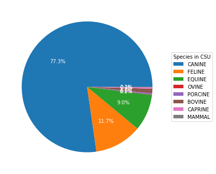
Figure S4: Species distribution in CSU dataset (left) and PP dataset (right).

Data Availability

The data that support the findings of this study are available from Colorado State University College of Veterinary Medicine, a private practice veterinary hospital near San Francisco and SAGE Centers for Veterinary Specialty & Emergency Care, but restrictions apply to the availability of these data, which were made available to Stanford for the current study, and so are not publicly available. Data are however available from the authors upon reasonable request and with permission of Colorado State University College of Veterinary Medicine, the private hospital and SAGE Centers for Veterinary Specialty & Emergency Care.

A.3 Result Details

We compute precision, recall, F1 and accuracy score for 20 most frequent disease categories. We list the results in Table S2.

	CSU				PP
Disease	P	R	$F_{1}$	N	P	R	$F_{1}$	N
Disorder of cellular component of blood	81	51	63	2263	50	43	46	7
Congenital disease	73	37	49	3345	50	12	19	17
Propensity to adverse reactions	75	81	78	5105	56	44	49	43
Metabolic disease	81	44	57	5265	57	46	51	26
Disorder of auditory system	85	64	73	5393	77	80	79	64
Hypersensitivity condition	82	80	81	6871	50	44	47	50
Disorder of endocrine system	81	70	75	7009	53	44	48	46
Disorder of hematopoietic cell proliferation	94	90	92	7294	67	50	57	16
Disorder of nervous system	80	62	70	7488	46	19	26	27
Disorder of cardiovascular system	88	49	63	8733	91	19	31	53
Disorder of the genitourinary system	85	58	69	8892	67	27	39	44
Traumatic AND/OR non-traumatic injury	71	67	69	9027	52	58	55	19
Visual system disorder	91	79	84	10139	77	55	64	62
Infectious disease	80	42	55	11304	70	30	42	88
Disorder of respiratory system	83	57	68	11322	47	26	33	27
Disorder of connective tissue	87	56	68	17477	78	29	42	24
Disorder of musculoskeletal system	87	61	72	20060	66	45	53	56
Disorder of integument	92	64	75	21052	77	49	60	156
Disorder of digestive system	76	68	72	22589	75	52	61	195
Neoplasm and/or hamartoma	95	85	90	36108	43	63	51	59

Table S2: Performance of the best model (Transformer+Auxiliary+Pretrain) for 20 most frequent disease categories.

To investigate the effectiveness of generative modeling pretraining and generative modeling as an auxiliary task, we compare the performance of two models: Transformer v.s. Transformer+Auxiliary+Pretrain on both CSU and PP datasets. We report precision, recall and F1 score for the 20 most frequent disease categories, as shown in Figure S5. We observe a significant improvement in recall for Transformer+Auxiliary+Pretrain model, which explains the overall improvement in F1 score.

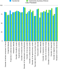
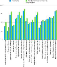
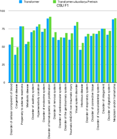
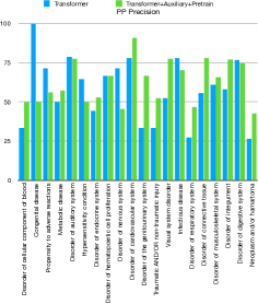
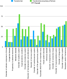
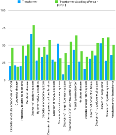
Figure S5: Performance comparison on the CSU and PP dataset for the 20 most frequent disease categories. Generative modeling pretraining and generative modeling as an auxiliary task improve recall significantly.

A.4 Interpretation Details

We use gradient-based interpretation attribution algorithm to compute the frequency of words that have score $\geq 0.2$ (threshold chosen heuristically), use MetaMap dictionary as a filter to extract medical relevant terms, and then sort them in decreasing order. We select the top 50 words and display words that intersect with the MetaMap expert-curated dictionary. We show results in Table S3, S4, S5. Disease categories without influential words are not shown.

Disease	Words
Disorder of	ear, otitis, ears, therapy, yeast,
auditory system	allergy, assessment, infection, weeks, malassezia,
	allergic, dermatology, this, disease, medications,
	dermatitis, left, has, avalanche, not,
	topical, drops,
Disorder of	eosinophilic, then, problem, todays, hypocalcemia,
immune function	cornea, dose, skin, alt, weeks,
	prednisolone, not, ofloxacin, eosinophilia, old,
	rhinitis, duration, currently, medicine, cam,
	cephalexin, molly, pancytopenia, hyperglobulinemia, herpes,
Metabolic disease	diabetes, nph, hypercalcemia, glargine, vetsulin,
	weeks, home, insulin, amlodipine, dose,
	dehydration, culture, eye, last, visit,
	assessment, time, oncology, cll, vet,
	azotemia, units, ionized, lymphoma, carprofen,
	consistent, surgery,
Autoimmune disease	pemphigus, itp, lupus, mycophenolate, azathioprine,
	not, weeks, bear, dle, planum,
	diagnosed, due, assessment, thrombocytopenia, administration,
	tramadol, home, platelet, mediated,
Disorder of	lymphoma, multicentric, chop, doxorubicin, assessment,
hematopoietic cell	trial, continued, lsa, chemotherapy, cbc,
proliferation	lymph, protocol, oncology, diagnosed, treatment,
	home, well, ccnu, weeks, remission,
Neoplasm and/or	oncology, lymphoma, osteosarcoma, sarcoma, mass,
hamartoma	home, carcinoma, assessment, metastatic, adenocarcinoma,
	chemotherapy, multicentric, tumor, trial, has,
	surgery, disease, time, diagnosed, carboplatin,
	well, weeks, pulmonary, melanoma, treatment,
	metastasis, palladia,
Disorder of	cardiology, hypertension, vasculitis, disease, current,
cardiovascular system	home, at, assessment, valve, amlodipine,
	atenolol, infection, pimobendan, sildenafil, thrombus,
	pressure, heart, blood, weeks, not,
	arrhythmia, ventricular, pulmonary, internal, failure,
	echocardiogram, time, iliac, hours,
Infectious disease	pyoderma, assessment, infection, bacterial, therapy,
	uti, urinary, culture, superficial, this,
	dermatitis, treat, today, secondary, infections,
	well, problem, time, urine, upper,
	chloramphenicol, allergies, but, weeks, site,
	home,
Disorder of	assessment, otitis, therapy, pyoderma, mct,
integument	vinblastine, dermatology, weeks, trial, home,
	has, malassezia, ear, problem, metastatic,
	allergic, this, atopic, not, eyelid,
	medications, mass,
Traumatic AND/OR	fracture, wound, laceration, due, assessment,
non-traumatic injury	trauma, this, bandage, time, owner,
	fractured, eye, surgery, fractures, she,
	days, dog, may, joint, abrasion,
	home, radiographs, likely, change,

Table S3: Most influential words in the best model (Transformer+Auxiliary+Pretrain). Disease categories without influential words are not shown.

Disease	Words
Disorder of	thrombocytopenia, pancytopenia, itp, time, mycophenolate,
cellular component	count, azathioprine, prednisone, tramadol, dose,
of blood	hemolytic, weeks, anemia, disease, leflunomide,
	steroids, eye, white, assessment, injury,
	future, problem, history, cbc,
Disorder of	pneumonia, pulmonary, lung, nasal, epistaxis,
respiratory system	adenocarcinoma, thoracocentesis, diagnosed, rhinitis, laryngeal,
	oncology, carcinoma, metastatic, paralysis, respiratory,
	assessment, home, mass, upper, revealed,
	necropsy, liver, consistent, chemotherapy, aspiration,
	srt, this, may, pneumothorax,
Vomiting	vomiting, ultrasound, chronic, assessment, findings,
	scan, skin, neoplasia, hematemesis, different,
	ddx, machine, nephrectomy, thickened, nodule,
	somewhat, ileum, not, intestines, last,
	bilateral,
Disorder of	laryngeal, seizures, his, meningioma, phenobarbital,
nervous system	seizure, home, signs, time, assessment,
	weeks, cytarabine, myelopathy, therapy, cricket,
	lesion, unremarkable, disease, hyperadrenocorticism, keppra,
	paralysis, tumor, neurology, levetiracetam, diagnosed,
	visit,
Hypersensitivity	dermatitis, allergic, therapy, atopic, otitis,
condition	pruritus, ears, assessment, allergies, dermatology,
	this, infection, weeks, treatment, not,
	ear, dvm, allergy, future, malassezia,
	time, today,
Anemia	pancytopenia, anemia, visit, hemolytic, persistent,
	steroids, hypertension, neoplasia, exam, thickening,
	calculi, white, inflammation, prednisolone, prednisone,
	treatments, vomiting, following, not,
Disorder of	bladder, assessment, hematuria, tcc, urinary,
the genitourinary	urethra, mass, culture, uti, pyelonephritis,
system	prostatic, cystitis, ureter, chemotherapy, diagnosed,
	testicle, therapy, piroxicam, disease, urine,
	not, prostate, revealed, carcinoma, renal,
	transitional, well, treatment, surgery,
Disorder of	thrombocytopenia, pancytopenia, itp, administration, prednisone,
hemostatic system	time, tramadol, bear, leflunomide, history,
	service, due, count, azathioprine, hypocalcemia,
	dose, mild, hypothyroidism, previous, steroids,
Propensity to	dermatitis, allergic, atopic, therapy, otitis,
adverse reactions	allergies, assessment, ears, infection, this,
	weeks, dermatology, pruritus, dvm, not,
	ear, trial, treatment, atopica, malassezia,
	atopy, today,
Poisoning	ingestion, assessment, toxicity, chocolate, vomiting,
	charcoal, not, maya, chance, activated,
	this, signs, dog, possible, rattlesnake,
	time, month, monitoring, therapy, marijuana,

Table S4: Most influential words in the best model (Transformer+Auxiliary+Pretrain). Disease categories without influential words are not shown.

Disease	Words
Mental disorder	alopecia, screen, limb, issue,
Congenital disease	dysplasia, hip, bilateral, assessment, testicle,
	right, cerebellar, service, surgery, echo,
	congenital, options, buffalo, mild, signs,
	butternut, malformation, worse, reverse, pain,
	deformity, red, elbow, management,
Disorder of	osteosarcoma, assessment, osteoarthritis, surgery, dysplasia,
musculoskeletal system	ligament, left, disease, carboplatin, oncology,
	time, right, at, rupture, trial,
	diagnosed, fracture, amputation, this, joint,
	bilateral, cruciate, she, chemotherapy, tendon,
	lesion, home, weeks, presented, osa,
Disorder of	methimazole, thyroid, weeks, levothyroxine, carcinoma,
endocrine system	mass, hyperadrenocorticism, assessment, diabetes, diagnosed,
	home, disease, nph, trilostane, dose,
	time, may, hyperthyroidism, surgery, visit,
	glargine, eye,
Disorder of	dental, assessment, sac, adenocarcinoma, melanoma,
digestive system	mass, home, has, anal, time,
	oncology, carboplatin, anesthesia, left, metastatic,
	disease, this, enteropathy, necropsy, problem,
	not, surgery, oral, lip, liver,
	enteritis, from,
Visual system	eye, ophthalmology, surgery, eyelid, assessment,
disorder	sicca, time, uveitis, diagnosed, this,
	keratitis, cataract, treatment, mass, glaucoma,
	after, week, well, months, visit,
	infection,
Disorder of	osteosarcoma, assessment, ligament, surgery, carboplatin,
connective tissue	disease, dysplasia, rupture, cruciate, fracture,
	amputation, hip, weeks, right, diagnosed,
	left, trial, osa, chemotherapy, anesthesia,
	this, tendon, bilateral, oncology, joint,
	crcl, she, well,
Disorder of	level, progesterone, high, apparently, assessment,
labor / delivery	draw, healthy, days, puppies,
Disorder of	progesterone, level, today, veterinary, measure,
pregnancy	high, labor, pregnant, approximately, assessment,
	healthy, prior, once,

Table S5: Most influential words in the best model (Transformer+Auxiliary+Pretrain). Disease categories without influential words are not shown.

References

- Ancona et al. (2018) Ancona, M.; Ceolini, E.; Oztireli, C.; and Gross, M. 2018. Towards better understanding of gradient-based attribution methods for deep neural networks. In 6th International Conference on Learning Representations (ICLR 2018).
- Aronson and Lang (2010) Aronson, A. R., and Lang, F.-M. 2010. An overview of metamap: historical perspective and recent advances. Journal of the American Medical Informatics Association 17(3):229–236.
- Baraban and Löscher (2014) Baraban, S. C., and Löscher, W. 2014. What new modeling approaches will help us identify promising drug treatments? In Issues in Clinical Epileptology: A View from the Bench. Springer. 283–294.
- Bird and Loper (2004) Bird, S., and Loper, E. 2004. Nltk: the natural language toolkit. In Proceedings of the ACL 2004 on Interactive poster and demonstration sessions, 31. Association for Computational Linguistics.
- Donnelly (2006) Donnelly, K. 2006. Snomed-ct: The advanced terminology and coding system for ehealth. Studies in health technology and informatics 121:279.
- Grimm (2016) Grimm, D. 2016. From bark to bedside.
- Hernandez et al. (2018) Hernandez, B.; Adissu, H. A.; Wei, B.-R.; Michael, H. T.; Merlino, G.; and Simpson, R. M. 2018. Naturally occurring canine melanoma as a predictive comparative oncology model for human mucosal and other triple wild-type melanomas. International journal of molecular sciences 19(2):394.
- Hochreiter and Schmidhuber (1997) Hochreiter, S., and Schmidhuber, J. 1997. Long short-term memory. Neural computation 9(8):1735–1780.
- Klinck et al. (2017) Klinck, M. P.; Mogil, J. S.; Moreau, M.; Lascelles, B. D. X.; Flecknell, P. A.; Poitte, T.; and Troncy, E. 2017. Translational pain assessment: could natural animal models be the missing link? Pain 158(9):1633–1646.
- Kol et al. (2015) Kol, A.; Arzi, B.; Athanasiou, K. A.; Farmer, D. L.; Nolta, J. A.; Rebhun, R. B.; Chen, X.; Griffiths, L. G.; Verstraete, F. J.; Murphy, C. J.; et al. 2015. Companion animals: Translational scientist’s new best friends. Science translational medicine 7(308):308ps21–308ps21.
- LeBlanc, Mazcko, and Khanna (2016) LeBlanc, A. K.; Mazcko, C. N.; and Khanna, C. 2016. Defining the value of a comparative approach to cancer drug development. Clinical Cancer Research 22(9):2133–2138.
- Mullenbach et al. (2018) Mullenbach, J.; Wiegreffe, S.; Duke, J.; Sun, J.; and Eisenstein, J. 2018. Explainable prediction of medical codes from clinical text. arXiv preprint arXiv:1802.05695.
- Pedregosa et al. (2011) Pedregosa, F.; Varoquaux, G.; Gramfort, A.; Michel, V.; Thirion, B.; Grisel, O.; Blondel, M.; Prettenhofer, P.; Weiss, R.; Dubourg, V.; Vanderplas, J.; Passos, A.; Cournapeau, D.; Brucher, M.; Perrot, M.; and Duchesnay, E. 2011. Scikit-learn: Machine learning in Python. Journal of Machine Learning Research 12:2825–2830.
- Radford et al. (2018) Radford, A.; Narasimhan, K.; Salimans, T.; and Sutskever, I. 2018. Improving language understanding by generative pre-training.
- Sennrich, Haddow, and Birch (2015) Sennrich, R.; Haddow, B.; and Birch, A. 2015. Neural machine translation of rare words with subword units. arXiv preprint arXiv:1508.07909.
- Sorower (2010) Sorower, M. S. 2010. A literature survey on algorithms for multi-label learning. Oregon State University, Corvallis 18.
- Vaswani et al. (2017) Vaswani, A.; Shazeer, N.; Parmar, N.; Uszkoreit, J.; Jones, L.; Gomez, A. N.; Kaiser, Ł.; and Polosukhin, I. 2017. Attention is all you need. In Advances in Neural Information Processing Systems, 5998–6008.