The Redshift Distribution of Infrared-Faint Radio Sources

Abstract

Infrared-Faint Radio Sources (IFRSs) are an important class of high-redshift active galaxy, and potentially important as a means of discovering more high-redshift radio sources, but only 25 IFRSs had redshifts prior to this paper. Here we increase the number of IFRSs with known spectroscopic redshifts by a factor of about 5 to 131, with redshifts up to $z=4.387$, and a median redshift of z = 2.68. The IFRS redshift distribution overlaps with the high-$z$ radio galaxy (HzRG) redshift distribution but is significantly narrower, suggesting that the IFRSs are a subset of the larger class of HzRGs. We also confirm and measure the proposed correlation between redshift and 3.6$\mu$m flux density, making it possible to use this correlation to find even higher redshift radio sources. Many more high-redshift sources are probably present in existing radio survey catalogues.

1 Introduction

Infrared-faint radio sources (IFRSs) are galaxies that are strong at radio wavelengths and weak in the infrared. Most are at high redshift, and selecting them represents a valuable technique for finding high-redshift radio sources. Although this class of objects is well-studied (Norris et al., 2006; Norris et al., 2007; Middelberg et al., 2008; Middelberg et al., 2010; Huynh et al., 2010; Zinn et al., 2011; Norris et al., 2011b; Collier et al., 2014; Garn & Alexander, 2008; Herzog et al., 2014, 2015a, 2015b; Herzog et al., 2016; Maini et al., 2016; Singh et al., 2014; Singh et al., 2017), their faintness at optical/IR wavelengths means that only 25 of them have measured spectroscopic redshifts, all but one of which are at redshift z $>$ 2.

Norris et al. (2006) first identified this class of source by cross-matching observations from the Australia Telescope Large Area survey (ATLAS) survey and the Spitzer Wide-Area Extragalactic (SWIRE; Lonsdale et al. 2003) survey. Out of the 2002 radio sources found by ATLAS in the Chandra Deep Field South (CDFS; Rosati et al. 2002) and European Large Area ISO Survey - South 1 (ELAIS-S1; Oliver et al. 2000) fields, only 53 were IFRSs, making them rare.

Norris et al. (2011b) suggested that IFRSs were most likely radio-loud active galactic nuclei (AGN) at high redshifts. They also considered the less likely possibility of IFRSs being radio-loud AGN at a redshift of $1<z<3$, with dust extinction reducing the luminosity.  Middelberg et al. (2010) compared the ratio of the 1.4 GHz and 3.6$\,\mu$m flux densities for an IFRS sample, a High-$z$ Radio Galaxy (HzRG) sample and a general radio source population sample (constructed from ATLAS catalogues), demonstrating that this ratio was common to the classes of IFRSs and HzRGs but not to the class of general radio sources.

Norris et al. (2007) detected an IFRS using Very Long Baseline Interferometry (VLBI), showing that the source was probably an AGN, since a VLBI detection implies brightness temperatures greater than $10^{6}$ K, which can only be generated by an AGN.  Middelberg et al. (2008) imaged an IFRS using VLBI, showing that the size, spectrum, radio and infrared luminosity were consistent with the properties of a high redshift compact steep-spectrum (CSS) source and inconsistent with the properties of a low redshift galaxy of low luminosity or a normal radio galaxy. Herzog et al. (2015a) used VLBI observations to show that the majority of IFRSs probably contain AGN.

While Norris et al. (2006) defined criteria for IFRSs that depended on survey sensitivity, Zinn et al. (2011) proposed generalised criteria that are survey-independent, so that they can be applied to all astronomical surveys. The Zinn et al. (2011) criteria are:

• A flux density ratio of $S_{\rm 20\,cm}/S_{\rm 3.6\,\mu m}>500$

• A 3.6$\,\mu$m flux density of $<30\,\mu$Jy

The first criterion selects sources with extreme infrared to radio flux density ratios, similar to HzRGs. The second criterion removes radio-loud AGN with low redshifts.

Using these criteria, Collier (2016) generated a sample of 1317 IFRSs, which included 93 compact steep-spectrum (CSS) sources and 31 GHz peaked-spectrum (GPS) sources. CSS are compact, powerful radio sources with a spectral peak at $\sim$100 MHz, while GPS have a spectral peak at $\sim$1 GHz  (Orienti, 2015). Using a sample of 14 IFRSs from the ELAIS-S1 and 14 from the CDFS, Herzog et al. (2016) determined that $\geq 15^{+8}_{-4}$ per cent of their sample were CSS sources and $3^{+6}_{-1}$ per cent were GPS sources. Singh et al. (2017) determined the radio morphologies of a sample of 11 IFRSs from the Subaru X-ray Deep Field (SXDF) and 8 from the Very Large Array - VIMOS VLT Deep Survey (VLA-VVDS) field. Of the total sample of 19 IFRSs, 14 were unresolved point sources and five featured extended double-lobed morphologies, classifying them as radio galaxies.

Finding high-redshift radio sources is important both as probes of the intergalactic medium, and as a means of studying the sub-kpc morphology of active galactic nuclei in the early Universe, including the possibility of detecting binary supermassive black holes. Previous attempts to find high-redshift radio sources have mainly used the apparent correlation between redshift and spectral index (e.g. Miley & De Breuck, 2008). Since virtually all IFRS are at z $>$ 2, they are potentially an even more efficient technique for finding high-redshift sources.

Determining the redshift of IFRSs is key to understanding their nature. Because of their faintness, very few redshifts have been measured.  Herzog et al. (2014) determined spectroscopic redshifts for three sources of $z$ = 1.84, 2.13 and 2.76. Of the 1317 IFRSs examined by Collier et al. (2014) from the Wide-field Infrared Survey Explorer  (WISE; Wright et al., 2010) All-Sky data release (Cutri et al., 2012), only 19 had spectroscopic redshifts listed in SDSS DR9. Remarkably, 18 of these had redshifts of z $\geq$ 2, suggesting that the IFRSs with spectroscopic redshift measurements are unlikely to be nearby AGN, but are more likely to be high-redshift AGN. As the majority of WISE sources have redshifts of $z<1$, these sources were very unlikely to be misidentifications.  Herzog et al. (2015a) also determined the photometric redshifts of 11 IFRSs observed with the Very Long Baseline Array. Three of these had spectroscopic redshift measurements listed in the Sloan Digital Sky Survey (SDSS) Data Release 10 (DR10) of $z$ = 2.11, 2.55 and 2.62, which had already been listed by Collier et al. (2014). Of the 19 IFRSs identified by Singh et al. (2017), only three had spectroscopic redshifts, which were $z$ = 2.43, 2.47 and 3.57. Obtaining spectroscopic redshifts for a larger sample of IFRSs is crucial to determine their true nature.

In this paper we do not distinguish between high-redshift radio galaxies and radio-loud quasars, which differ intrinsically only by their orientation (Urry & Padovani, 1995), as we are primarily concerned with the flux density at 20 cm and 3.6 $\mu\mathrm{m}$. At mJy sensitivities, the flux of most radio galaxies is dominated by hotspot and lobe emission, and so (with the exception of the relatively rare flat-spectrum quasars and blazars) is independent of orientation, and so radio galaxies and quasars with similar host properties have similar flux densities (e.g. Urry & Padovani, 1995).

The orientation dependence at 3.6 $\mu\mathrm{m}$ is less well-defined, since this corresponds to a rest wavelength of 1.8–0.7 $\mu\mathrm{m}$ for the redshift range z $\sim$ 1–4 of our sample. At these wavelengths, the emission will contain contributions from the accretion disc, dusty torus, and the host galaxy, with the importance of the accretion disc, and extinction by the torus, increasing at shorter wavelengths (Hernán-Caballero et al., 2016), leading to some orientation dependence. However, the optical spectra, at even shorter wavelengths, are even more strongly affected by the orientation, making quasars more easily observable in spectroscopy than radio galaxies. Therefore, IFRSs with measured redshifts are much more likely to be quasars than IFRSs without measured redshifts. As a result, the majority of IFRSs discussed in this paper, and in papers such as Herzog et al. (2014), are quasars. However their radio and infrared properties are similar to those of radio galaxies, which probably constitute the majority of the IFRSs.

The goal of this paper is to obtain a larger sample of IFRSs with spectroscopic redshifts. Section 2 of this paper introduces our dataset. Section 3 presents our redshift distribution. Section 4 discusses the redshift distribution and Section 5 presents our conclusions.

2 Data

Our data were selected following a procedure similar to Collier et al. (2014), using deeper photometry from WISE and more extensive spectroscopy from SDSS.

Our IFRS sample was taken from Version 2.0 of the Unified Radio Catalog  (URC; Kimball & Ivezić, 2008; Kimball & Ivezic, 2014). This catalog contains approximately three million radio sources, and combines the 20 cm flux density measurements from the Faint Images of the Radio Sky at Twenty Centimeters (FIRST; Becker et al. 1995) survey and the NRAO-VLA Sky Survey (NVSS; Condon et al. 1998).

We obtained infrared data from the AllWISE data release (Cutri et al., 2014), which improves upon the sensitivity, photometric and astrometric accuracy of the WISE All-Sky data release. We converted 3.4$\,\mu$m measurements from magnitudes to Jansky (Jy) with a flat color correction factor, using the conversion determined for IFRSs by Collier et al. (2014):

$$S_{3.4\,{\mu}\mathrm{m}}=306.682\times 10^{(-M_{3.4\,\mu\mathrm{m}}/2.5)}Jy$$ (1)

We used spectroscopic redshifts from SDSS DR12 (Alam et al., 2015). DR12 contains measurements from 2008 to 2014, taken by the third generation of SDSS.

2.1 Selection Criteria

In Table 1, we present the selection criteria followed to select our sample, and the number of sources remaining after applying each criterion, which we now explain in more detail:

1. We began with the 2,866,856 sources from the URC v2.0.

2. We applied a NVSS flux density limit of $S_{\rm 20\,cm}$ > 7.5 mJy. This was applied to reduce the size of the following WISE query, since all IFRSs with $S_{\rm 20\,cm}/S_{\rm 3.4\,\mu m}>500$ will have $S_{\rm 20\,cm}$ > 7.5 mJy, following a 5$\sigma$ detection and an r.m.s. of $\sigma>3\,\mu$Jy at 3.4 $\,\mu$m.

3. We removed all sources that did not have at least one FIRST counterpart, which we used for the radio source positions, as FIRST has a higher angular resolution than NVSS.

4. We cross-matched the FIRST positions to AllWISE. We used a search radius of 5 arcsec to ensure minimal false matches at redshifts of $z>0.5$.

5. We applied the second of Zinn et al. (2011)’s generalised IFRS criteria, $S_{\rm 20\,cm}/S_{\rm 3.4\,\mu m}>500$.

6. We applied a 3.4$\,\mu$m signal-to-noise ratio (SNR) limit of $\geq 5$.

7. We cross-matched our sources to SDSS DR12 using the AllWISE positions and a search radius of 1 arcsec.

8. We selected all sources with spectroscopic redshifts.

9. We removed all duplicate sources that shared the same SDSS optical spectroscopic object identification number.

10. We removed all sources with a spectral classification of a STAR, ensuring all sources were extragalactic.

11. We removed all sources with redshift warning flags.

12. We removed all sources with negative redshift errors, as for these sources, the errors could not be determined.

13. We selected all sources that had Q (observation quality) values of 3 for good, as opposed to 1 for bad or 2 for acceptable.

14. We applied the first of  Zinn et al. (2011)’s generalised IFRS criteria, $S_{\rm 3.4\,\mu m}<30\,\mu$Jy, resulting in our IFRS sample.

15. We visually inspected an image of each IFRS, using the AllWISE 3.4$\,\mu$m and SDSS $i$ band images and FIRST contours, such as the one shown in Figure 1. No sources were identified as misidentifications.

After we applied the first 12 selection criteria, our sample consisted of 2521 radio sources with spectroscopic redshifts from SDSS. We call this our “initial large sample”. After applying all 14 criteria, our sample consisted of 108 IFRSs, and we call this our “IFRS sample”. Two of these sources already had spectroscopic redshifts listed by Collier et al. (2014).

Table 1: The selection criteria and number of sources after applying each criterion to our IFRS sample.

No.	Selection Criterion	Sources
0	Total Unified Radio Catalog	2,866,856
1	NVSS flux density $S_{\rm 20\,cm}>7.5$ mJy	1,139,132
2	At least one FIRST counterpart	621,316
3	AllWISE match within 5$\arcsec$ of FIRST	303,043
4	$S_{\rm 20\,cm}/S_{\rm 3.4\,\mu m}>500$	64826
5	$S_{\rm 3.4\,\mu m}$ SNR $>=5$	63998
6	SDSS match within 1$\arcsec$ of AllWISE	46490
7	SDSS source with Spectroscopic Redshift	5761
8	Remove SDSS duplicates	2798
9	Not a star	2747
10	No zWarning flag	2566
11	Positive z Error	2551
12	Good quality observation	2521
13	$S_{\rm 3.4\,\mu m}<30\,\mu$Jy	108
14	Visual Inspection of images and spectra	108

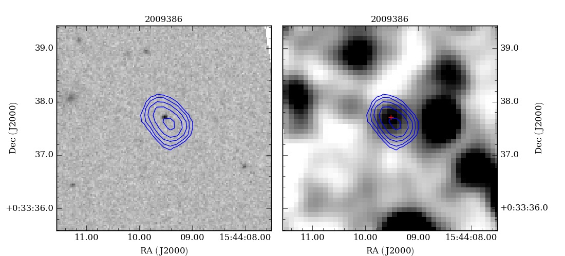
Figure 1: An example postage stamp of an IFRS, generated for visual inspection. FIRST contours are shown in blue, representing 4-1024 times the local r.m.s., increasing by multiples of 2, overlaid on the the SDSS $i$ band image (left), and the AllWISE 3.4$\,\mu$m image (right). The red cross in the right image shows the position of the SDSS fibre used to measure the redshift. Both panels are labelled according to their unique ID from the URC.

2.2 Positional Offsets

We show positional offsets of the sources in our IFRS sample between FIRST and ALLWISE and between ALLWISE and SDSS in Figure 2, and display their median and mean values in Table 2. This shows there are no significant systematic offsets.

Table 2: The positional offsets in arcsec between our datasets

	Radial Separation	RA	Dec
FIRST–AllWISE Median	0.87	0.58	0.47
FIRST–AllWISE Mean	1.05	0.74	0.60
AllWISE–SDSS Median	0.59	0.30	0.34
AllWISE–SDSS Mean	0.61	0.39	0.38

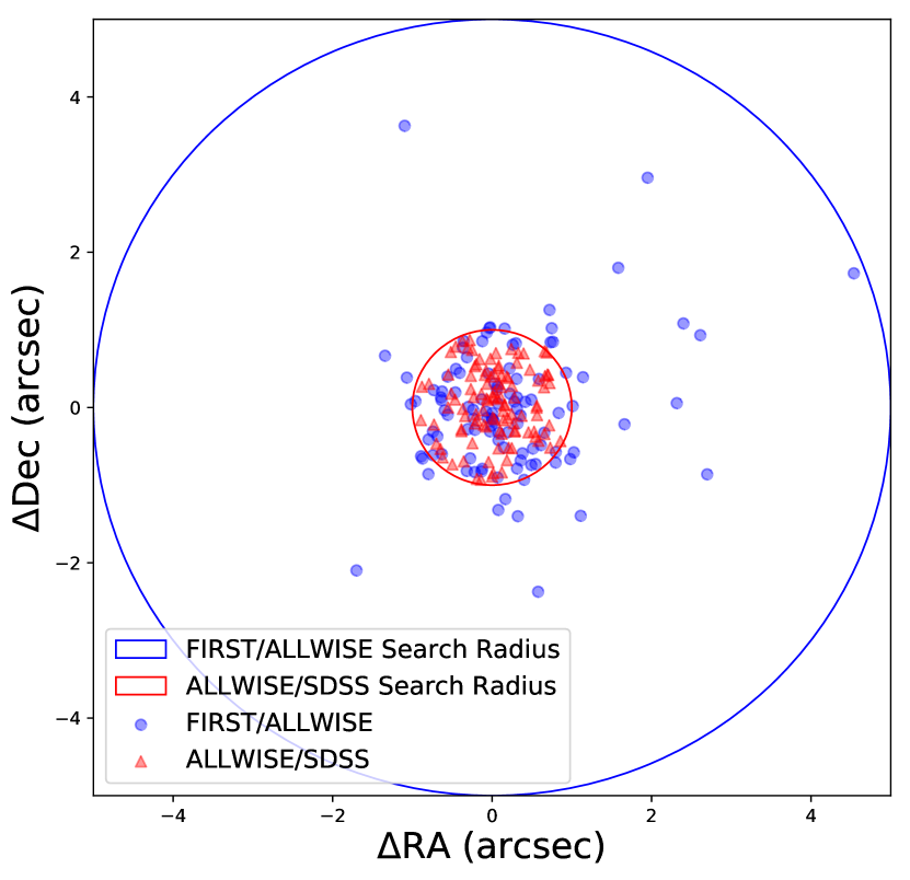
Figure 2: The sky separations for our 108 IFRSs with spectroscopic redshifts, between FIRST and AllWISE (blue circles) and AllWISE and SDSS (red triangles). The FIRST–AllWISE search radius of 1$\arcsec$ is shown in red, and the AllWISE–SDSS search radius of 5$\arcsec$ is shown in blue.

2.3 Misidentification Rates

To estimate the misidentification rate, particularly due to confusion within the AllWISE catalogue, we downloaded a subset of the URC, AllWISE and SDSS catalogues from two regions of sky, given the non-uniformity of these surveys. Region one was constrained to one degree either side of a position of (5,5) degrees (i.e. 00:16:00 $\leq$ RA $\leq$ 00:24:00, and $4\deg\leq$ Dec $\leq 6\deg$), while region two was constrained to one degree either side of a position of (10,10) degrees (i.e. 00:36:00 $\leq$ RA $\leq$ 00:44:00, and $9\deg\leq$ Dec $\leq 11\deg$). We shifted the positions of all of the FIRST sources by a single random amount between either $-$60 to $-$20 arcsec or 20 to 60 arcsec. These shift sizes were chosen to be greater than the beam sizes for the FIRST, AllWISE and SDSS surveys. We then cross-matched FIRST to AllWISE with a search radius of 5$\arcsec$. We applied the selection criteria shown in Table 1 to the shifted sources. For computational reasons, the criteria were applied in a slightly different order than had been used on the original sample. Lastly, we cross-matched AllWISE to the SDSS spectroscopic redshift catalogue of that region, with a search radius of 1$\arcsec$. This process was repeated 1000 times, each time shifting all FIRST positions by a different random amount.

We determined the misidentification rate by dividing the mean number of shifted cross-matches by the number of unshifted cross-matches. The result is shown in Table 3, which shows that, after all criteria have been applied, essentially none of the selected sources, in either the large sample or the IFRS sample, are erroneous.

Table 3: The misidentification rates for survey cross-matches

Selection Criteria	Rate (%)	Rate (%)
	region 1	region 2
AllWISE match within 5$\arcsec$ of FIRST	18.2	18.1
NVSS flux density $S_{\rm 20\,cm}>7.5$ mJy	5.5	5.7
$S_{\rm 20\,cm}/S_{\rm 3.4\,\mu m}>500$	1.6	2.2
$S_{\rm 3.4\,\mu m}$ SNR $>=5$	1.6	2.2
SDSS spec match within 1$\arcsec$ of AllWISE	0.00	0.01

Misidentification rates calculated by randomly shifting sources in two regions, as described in the text. The rate shown is the median number in the shifted sample that satisfy the criteria, divided by the number in an unshifted sample that satisfy the criteria.

3 Redshift Distribution

3.1 The Large Sample of Radio Sources

There are three sources in our initial large sample with redshifts of $z\geq 5$.

When we examined the SDSS spectra for them, we found that in two cases (SDSS J105631.94-01145.1 and SDSS J111036.32+481752.3), the redshift depended almost entirely on a single line which was identified as Lyman-$\alpha$, but which had no corroborating evidence, such as a Lyman break, and there were other strong unidentified lines, making it resemble the spectrum of a low-redshift galaxy. We thus chose to exclude these two sources from further consideration, reducing the size of our initial large sample to 2519 sources, which we call our “large sample”. The sample of 108 IFRS is not affected by this.

The large sample of 2519 sources is available as supplementary information in the online version of this paper, and a sample of the first few rows of this Table is shown in Table 4.

Table 4: The first 5 and the last 5 rows of our large sample. The full table is available as supplementary information in the online version of this paper.

ID	RA	Dec	$S_{20cm}$	$S_{3.4\mu m}$	z	$\delta$z
1	221.68050	27.95017	1113.9	303.3	0.00692	0.00007
2	229.18569	7.02204	5499.3	8635.5	0.03453	0.00001
3	117.03940	30.10852	225.5	324.7	0.04209	0.00001
4	152.00014	7.50458	6522.1	149.8	0.06813	0.00004
5	9.26650	-1.15124	4067.1	4420.7	0.07365	0.00001
2515	243.06980	47.04826	53.5	72.8	4.36238	0.00072
2516	233.89124	2.90653	59.5	25.1	4.38719	0.00129
2517	145.02005	5.44189	61.7	39.9	4.50384	0.00055
2518	210.10587	31.81968	21.9	41.7	4.69133	0.00053
2519	156.59841	25.71657	256.9	65.6	5.27746	0.00064

Column descriptions:
1: Unique ID from 1-2519
2: FIRST (Becker et al. 1995) Right Ascension (J2000) in degrees
3: FIRST (Becker et al. 1995) Declination (J2000) in degrees
4: NVSS (Condon et al. 1998) 20 cm radio flux density in mJy
5: AllWISE (Cutri et al. 2013) 3.4 $\mu$m infrared flux density in $\mu$Jy
6: SDSS DR12 (Alam et al. 2015) spectroscopic redshift
7: Mean SDSS DR12 (Alam et al. 2015) spectroscopic redshift error

In the remaining high-redshift galaxy, SDSS J102623.62+254259.6, the identification of the putative Lyman-$\alpha$ line was confirmed by the presence of a strong Lyman break. SDSS J102623.62+254259.6 is therefore a radio-loud quasar at a redshift of 5.28, making it one of the highest-redshift radio-loud sources known.

Two other sources (SDSS J151656.6+183021 = 3C316, and SDSS J101115.64+010642.5 = PKS 1008+013) had large but unreliable redshifts listed by SDSS, and modest but reliable redshifts from other authors, and so their redshifts were corrected in our database.

In Figure 3 we plot the $S_{3.4{\mu}\mathrm{m}}$ flux density of the 2519 galaxies in the large sample as a function of redshift. This is discussed further in Section 4.2 below.

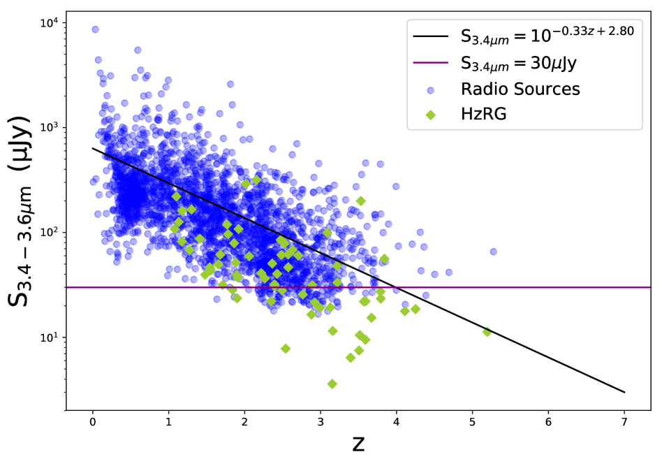
Figure 3: The $S_{3.4-3.6{\mu}\mathrm{m}}$ flux density as a function of $z$, the spectroscopic redshift, for our selected radio sources, plotted as blue circles, and the HzRGs from Seymour et al. (2007), plotted as green diamonds. The sources clearly follow an IR-$z$ correlation which, as suggested by Norris et al. (2011b), might yield even higher redshift sources by correlating radio surveys with higher sensitivity infrared surveys. Our IFRS sample consists of the 108 blue circles that lie below the horizontal line marking the 30 $\mu$Jy flux density limit.

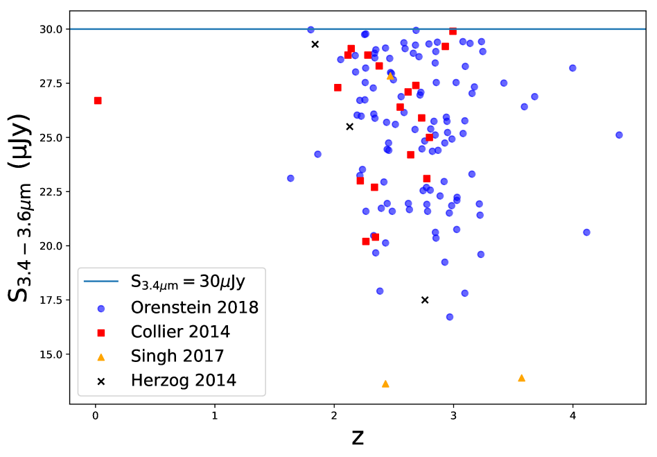
Figure 4: The $S_{3.4-3.6{\mu}\mathrm{m}}$ flux density as a function of $z$, the spectroscopic redshift, for our sample of 108 IFRSs, plotted as blue circles, the IFRSs from Collier et al. (2014), plotted as red squares, the IFRSs from Singh et al. (2017), plotted as orange triangles, and the IFRSs from Herzog et al. (2014), plotted as black crosses. Sources from Herzog et al. (2015a) are not shown since they are a subset of those already identified in Collier et al. (2014).

3.2 IFRSs

After we applied the entire 14 selection criteria, our sample consisted of 108 IFRSs (106 of which are new) with spectroscopic redshifts from SDSS, listed in Table LABEL:table:IFRSs. We plot their $S_{3.4{\mu}\mathrm{m}}$ flux densities as a function of redshift in Figure 4. For comparison, we also show the IFRS samples from Collier et al. (2014), Herzog et al. (2014), and Singh et al. (2017).

There is a clear overlap between the samples, and a high density of IFRSs up to the $S_{\rm 3.4\,\mu m}<30\,\mu$Jy cutoff. Nearly all IFRSs in these samples lie between two sharply defined boundaries at about $z$ = 2.4 and $z$ = 3.4. However, Figure 3 shows that these boundaries are caused by the intersection of the IR-$z$ correlation and our IR flux limit.

4 Discussion

4.1 The IFRS Sample

Before the present work, only 25 IFRSs had measured spectroscopic redshifts (Collier et al., 2014; Herzog et al., 2014; Singh et al., 2017), with a maximum redshift of 3.570. Our sample gives a fivefold increase in the number of IFRS with spectroscopic redshifts, adding 106 sources, and raises the maximum redshift to 4.387 (ID 86 in Table LABEL:table:IFRSs).

4.2 Confirming the Flux Density – Redshift Correlation

In Figure 3 we plot the $S_{\rm 3.4\,\mu m}$ flux density of the 2519 galaxies in the large sample as a function of redshift. For comparison, we also show the 69 High-$z$ Radio Galaxies (HzRGs) from  Seymour et al. (2007). It is clear from this plot that the galaxies show the inverse correlation between 3.6$\,\mu$m flux density and redshift first noted by Norris et al. (2011b).

This correlation, which is similar to the well-known $k-z$ relation (Willott et al., 2003), was confirmed by  Singh et al. (2017) for all known IFRSs and the Seymour et al. (2007) sample of HzRGs. With the much larger number of sources now available, we confirmed and refined this correlation by fitting a straight-line to the data in log-lin space. We used the Levenberg-Marquardt algorithm (Moré, 1978) to perform a nonlinear least-squares fit with SciPy (Jones et al., 2001), and obtained the relation:

$$S_{\rm 3.4\,{\mu}m}=10^{-0.33(\pm 0.02)z+2.80(\pm 0.02)}$$ (2)

This is shown as the black line in Figure 3.

This correlation (hereafter called the IR-$z$ correlation) shows that, as suggested by Norris et al. (2011b), even higher redshift sources might be found by correlating radio surveys with even higher sensitivity infrared surveys.

4.3 Redshift distribution

In Figure 4.3 we plot the redshift distribution of the HzRGs from Seymour et al. (2007), the SDSS Quasar Catalog twelfth data release (SDSS DR12Q) pipeline redshift estimates Pâris et al. (2017), our IFRSs and a random 10 per cent of SDSS DR12 sources with spectroscopic redshifts. The HzRGs have a median redshift of $z=2.13$, and a wide redshift distribution consistent with that noted by Seymour et al. (2007).

The IFRSs in our sample have a narrower redshift distribution, with a median redshift of $z=2.68$. As would be expected, the majority of the SDSS sample contains lower redshifts, with a median redshift of $z=0.32$ and 87.50 per cent of the redshifts less than 1, clearly eliminating the possibility that IFRSs are misidentifications.

Figures 3 and 4 show that the redshift distribution of our IFRS sample is defined by the intersection of the IR-$z$ correlation with our IR flux density limit.

4.4 Using IFRSs to find high-z radio sources

Obtaining a census of high-redshift radio sources is important for several reasons.

First, conventional hierarchical models of the formation of super-massive black holes (SMBHs) are unable to produce such high-mass black holes early in the lifetime of the Universe, driving the development of novel models for supermassive black hole formation (e.g. Volonteri & Rees, 2005). HzRGs represent a subset of high-redshift super-massive black holes that are relatively easy to detect in large radio surveys, although measuring their redshifts is challenging. Finding a significant number of HzRGs at $z>6$ would exacerbate the problem of the formation of SMBHs at high redshift.

Second, high redshift radio sources are important cosmological probes, as they provide background sources against which HI absorption may be seen at high redshifts (Carilli et al., 2002; Ciardi et al., 2015)

If radio galaxies continue to follow the IR-$z$ correlation shown in Figure 3 to high redshift, then in principle HzRGs may be found by searching for radio sources with low IR flux densities. Such sources may already exist in current radio catalogues, and a great many more will be available from next-generation radio surveys (Norris, 2017) such as Evolutionary Map of the Universe (EMU; Norris et al., 2011a), MeerKAT International GHz Tiered Extragalactic Exploration Survey (MIGHTEE; Jarvis et al., 2017), the VLA Sky Survey(VLASS; Murphy & Vlass Survey Science Group, 2015), and the LOFAR Two-metre Sky Survey (LoTSS; Shimwell et al., 2017).

However, there are two potential challenges to be overcome to achieve this.

First, the sample shown in Figure 3 is limited by the sensitivity of the WISE survey. To detect sources at higher $z$, we need more sensitive infrared data. The SERVS survey (Mauduit et al., 2012) reaches an r.m.s. sensitivity at 3.6$\,\mu$m of about 0.2 $\mu$Jy, so that 5$\sigma$ SERVS detections should extend to about $z=7$. Because of strong radio source evolution (e.g. Norris et al., 2013), such sources may still be well above the radio detection limit.

However, the SERVS survey only covers a few tens of square degrees, limiting the number of high-$z$ IFRSs that can be detected (Maini et al., 2016). No other infrared survey in the near future will provide the required sensitivity over a large area of sky, although it is possible that $K$-band surveys such as the Vista Hemisphere Survey (VHS; McMahon et al., 2013), UKIRT Infrared Deep Sky Survey (UKIDSS; Lawrence et al., 2007) and VISTA Kilo-degree Infrared Galaxy Survey (VIKING; Edge et al., 2013) may be used for the same purpose together with corresponding radio surveys.

Second, we need to measure redshifts for these sources. Future large spectroscopic surveys such as 4MOST (Quirrenbach & Consortium, 2015), WEAVE-LOFAR (Smith et al., 2016), DESI (Levi et al., 2013), and PFS (Takada et al., 2014) may be able to provide this data, but the faintest sources will still be difficult to access at optical wavelengths. Potential alternatives include photometric redshift techniques, although these will be limited by the faintness of the optical/IR emission, or using blind scans for CO emission using ALMA (e.g. Weiß et al., 2013).

5 Conclusion

From cross-matching FIRST, AllWISE and SDSS DR12, we have compiled a large sample of 108 IFRSs with spectroscopic redshift measurements, greatly extending the previous sample of 25. This new sample includes the highest identified IFRS spectroscopic redshift with $z=4.387$. This sample will be valuable in future multi-wavelength studies, with high-angular-resolution radio imaging, to study the properties of IFRSs and determine what they can tell us about the evolution of AGN.

We have also shown that IFRSs, as well as a large sample of 2519 high-redshift radio sources with spectroscopic redshifts, follow a correlation of 3.4$\,\mu$m flux density as a function of redshift, with the form $S_{\rm 3.4\,{\mu}m}=10^{-0.33(\pm 0.02)z+2.80(\pm 0.02)}$. By extending this correlation to even fainter mid-infrared flux densities, this correlation appears to be a powerful tool for finding high-redshift radio sources, rivalling the use of steep-spectral index.

Future detections of high-redshift radio sources will be important for probing the high-redshift Universe, and to understand SMBH formation and AGN evolution. Future large radio surveys are likely to yield many such sources, provided that we have matching deep infrared photometry and a means of measuring redshifts.

6 Acknowledgements

We thank Dr. Rob Sharp for invaluable advice on SDSS spectroscopy, and Prof. Tom Jarrett for help with interpreting WISE flux densities.

We gratefully acknowledge the people and institutes that contributed to the NVSS and FIRST surveys.

This research has made use of Version 2.0 of the Unified Radio Catalog, (URC; Kimball & Ivezić, 2008; Kimball & Ivezic, 2014). The URC v2.0 website is http://www.aoc.nrao.edu/~akimball/radiocat_2.0.shtml.

This research has made extensive use of the NASA/IPAC Extragalactic Database (NED) which is operated by the Jet Propulsion Laboratory, California Institute of Technology, under contract with the National Aeronautics and Space Administration.

This research has made use of the VizieR catalog access tool, CDS, Strasbourg, France. Topcat (Taylor, 2005), NASA’s Astrophysics Data System bibliographic services, and Astropy, a community-developed core Python package for Astronomy (The Astropy Collaboration et al., 2018), were also used in this study.

This research made use of APLpy, an open-source plotting package for Python (Robitaille & Bressert, 2012).

This research made use of the Jupyter Notebook environment (Kluyver et al., 2016) and the Seaborn data visualisation library (Waskom et al., 2014).

This research made use of the following software in the SciPy (Jones et al., 2001) ecosystem: Numpy (Oliphant, 2015), iPython (Perez & Granger, 2007), Matplotlib (Hunter, 2007) and Pandas (McKinney, 2010).

This research made use of Montage. It is funded by the National Science Foundation under Grant Number ACI-1440620, and was previously funded by the National Aeronautics and Space Administration’s Earth Science Technology Office, Computation Technologies Project, under Cooperative Agreement Number NCC5-626 between NASA and the California Institute of Technology.

Funding for the Sloan Digital Sky Survey IV has been provided by the Alfred P. Sloan Foundation, the U.S. Department of Energy Office of Science, and the Participating Institutions. SDSS-IV acknowledges support and resources from the Center for High-Performance Computing at the University of Utah. The SDSS website is https://www.sdss.org.

SDSS-IV is managed by the Astrophysical Research Consortium for the Participating Institutions of the SDSS Collaboration including the Brazilian Participation Group, the Carnegie Institution for Science, Carnegie Mellon University, the Chilean Participation Group, the French Participation Group, Harvard-Smithsonian Center for Astrophysics, Instituto de Astrofísica de Canarias, The Johns Hopkins University, Kavli Institute for the Physics and Mathematics of the Universe (IPMU) / University of Tokyo, Lawrence Berkeley National Laboratory, Leibniz Institut für Astrophysik Potsdam (AIP), Max-Planck-Institut für Astronomie (MPIA Heidelberg), Max-Planck-Institut für Astrophysik (MPA Garching), Max-Planck-Institut für Extraterrestrische Physik (MPE), National Astronomical Observatories of China, New Mexico State University, New York University, University of Notre Dame, Observatário Nacional / MCTI, The Ohio State University, Pennsylvania State University, Shanghai Astronomical Observatory, United Kingdom Participation Group, Universidad Nacional Autónoma de México, University of Arizona, University of Colorado Boulder, University of Oxford, University of Portsmouth, University of Utah, University of Virginia, University of Washington, University of Wisconsin, Vanderbilt University, and Yale University.

This publication makes use of data products from the Wide-field Infrared Survey Explorer, which is a joint project of the University of California, Los Angeles, and the Jet Propulsion Laboratory/California Institute of Technology, and NEOWISE, which is a project of the Jet Propulsion Laboratory/California Institute of Technology. WISE and NEOWISE are funded by the National Aeronautics and Space Administration.

Table 5: Our sample of 108 IFRSs with spectroscopic redshift measurements

ID	SDSS ID	FIRST RA	FIRST Dec	$S_{\mathrm{20\,cm}}$	$S_{3.4\,\mathrm{{\mu}m}}$	$z$	$\pm z$
		(J2000)	(J2000)	(mJy)	($\mathrm{{\mu}Jy}$)		($10^{-3}$)
1	J004842.69+000543.7	12.17789	0.09539	30.69	29.94	2.69	0.27
2	J012753.69+002516.4	21.97376	0.42131	91.46	24.75	2.46	0.10
3	J014934.63-024305.3	27.39430	-2.71818	20.26	26.03	2.19	0.70
4	J020553.54-001338.7	31.47305	-0.22738	13.42	22.69	2.77	0.78
5	J025139.59-083432.5	42.91476	-8.57575	69.12	24.75	2.93	0.77
6	J025808.78-020912.7	44.53675	-2.15349	17.99	28.67	2.34	0.41
7	J073459.45+420425.4	113.74677	42.07347	20.66	26.74	2.26	0.55
8	J074013.97+463853.9	115.05820	46.64835	27.67	28.59	2.05	1.20
9	J074105.87+294909.7	115.27448	29.81936	33.50	25.74	2.84	0.32
10	J074950.69+191152.5	117.46117	19.19794	19.91	26.88	2.56	0.14
11	J080541.11+512707.4	121.42130	51.45205	27.72	26.15	2.59	0.54
12	J081553.19+063858.4	123.97165	6.64958	25.03	27.51	3.42	0.46
13	J081948.76+452434.1	124.95320	45.40952	34.08	25.39	2.81	0.26
14	J082617.09+362115.6	126.57134	36.35435	18.64	28.78	2.18	0.45
15	J083221.85+313518.4	128.09043	31.58768	54.53	22.57	2.80	0.80
16	J083935.95+011214.5	129.89975	1.20408	17.50	28.44	2.85	0.52
17	J083955.38+025145.4	129.98063	2.86267	78.60	26.88	3.68	0.23
18	J084423.07+523920.3	131.09626	52.65560	12.54	22.24	3.03	0.39
19	J085157.78+442107.9	132.99075	44.35220	12.87	24.93	2.99	0.30
20	J090259.94+272028.2	135.74976	27.34119	83.35	29.37	2.58	0.30
21	J093450.93+460329.0	143.71228	46.05806	13.46	23.52	2.24	0.50
22	J093536.18+291710.8	143.90071	29.28636	50.01	28.00	2.47	0.62
23	J094523.07+365555.5	146.34615	36.93206	36.54	29.13	2.43	0.42
24	J094705.51+302008.5	146.77299	30.33567	47.71	25.77	3.09	0.48
25	J095043.72+594631.2	147.68208	59.77535	11.71	19.60	3.23	0.28
26	J100653.88+595519.6	151.72447	59.92216	14.80	20.36	2.85	0.45
27	J100655.80+050324.8	151.73256	5.05686	29.57	29.42	3.08	0.71
28	J101032.23+080805.2	152.63407	8.13474	20.49	27.28	2.33	0.68
29	J102503.59+390350.1	156.26502	39.06389	26.97	24.45	2.44	0.53
30	J102823.47+500913.9	157.09777	50.15408	14.30	26.96	2.72	0.97
31	J102846.94+412656.7	157.19568	41.44908	71.99	24.36	2.82	0.54
32	J111141.06+562503.5	167.92120	56.41775	65.04	25.60	2.51	0.45
33	J111636.11+583231.0	169.15048	58.54193	19.92	27.54	2.85	0.34
34	J111658.03+520333.5	169.24183	52.05913	29.56	28.89	2.34	0.30
35	J112341.85+091328.4	170.92440	9.22458	20.08	29.75	2.25	0.37
36	J112344.71+342546.7	170.93641	34.42975	14.75	27.03	3.15	0.25
37	J112356.35+462901.2	170.98462	46.48382	31.36	26.71	2.21	0.45
38	J112549.64+482759.6	171.45682	48.46654	24.48	28.20	4.00	0.40
39	J113116.45+514634.2	172.81872	51.77623	93.67	25.74	2.94	0.37
40	J113605.23+222218.2	174.02162	22.37173	32.83	28.28	3.10	0.18
41	J113610.45+314924.9	174.04336	31.82377	15.26	29.31	2.79	0.77
42	J113902.81+231016.7	174.76174	23.17148	44.45	28.65	2.47	0.26
43	J113904.76+245712.1	174.76979	24.95311	30.08	28.20	2.26	0.36
44	J115428.30+141004.2	178.61794	14.16786	14.70	29.26	2.68	0.29
45	J115650.86+353103.5	179.21206	35.51766	197.38	29.34	3.14	0.59
46	J121129.17+243958.9	182.87153	24.66634	25.00	27.54	3.02	0.63
47	J121230.17+251321.2	183.12567	25.22255	216.33	24.41	2.87	0.81
48	J121840.03+244955.0	184.66686	24.83194	239.19	28.97	2.85	0.18
49	J122046.01+494508.4	185.19181	49.75238	14.94	24.84	2.76	2.00
50	J124541.71+255918.0	191.42293	25.98868	15.02	29.78	2.26	0.24
51	J125134.74+581257.6	192.89482	58.21599	13.79	19.24	2.93	1.07
52	J125230.57+245813.3	193.12733	24.97042	14.27	27.94	2.48	0.66
53	J125300.15+524803.3	193.25067	52.80096	58.02	20.62	4.12	0.53
54	J125656.83+385540.2	194.23691	38.92792	18.08	21.95	2.44	0.70
55	J125832.23+454305.1	194.63454	45.71699	13.56	22.95	2.42	0.90
56	J130417.79+564729.9	196.07378	56.79157	12.32	20.13	2.43	0.46
57	J130744.40+212615.5	196.93514	21.43769	98.70	24.41	2.46	0.31
58	J132622.76+582750.1	201.59474	58.46398	44.54	21.85	2.98	0.84
59	J133202.45+211317.8	203.01015	21.22149	14.56	27.33	3.17	0.31
60	J133221.80-022449.7	203.09031	-2.41391	29.54	28.97	3.24	0.35
61	J133714.92+352958.5	204.31208	35.49965	33.72	28.73	2.71	0.43
62	J134329.90+320800.2	205.87462	32.13342	19.54	23.31	3.15	0.30
63	J134637.43+290042.4	206.65597	29.01181	36.48	27.08	2.73	0.15
64	J140828.37+060902.9	212.11765	6.15066	19.43	25.89	2.34	0.33
65	J141204.71+282237.7	213.01962	28.37714	35.16	27.66	2.50	0.17
66	J141309.25+240700.6	213.28852	24.11682	20.56	29.05	2.35	0.49
67	J141529.73-021448.2	213.87350	-2.24708	16.07	23.24	2.21	0.29
68	J141637.23+143044.2	214.15515	14.51232	134.11	21.59	2.78	1.44
69	J143130.84+233422.2	217.87853	23.57281	23.62	26.42	3.59	0.37
70	J143243.17+232009.4	218.17992	23.33607	14.66	22.30	2.89	0.67
71	J143301.51+010132.9	218.25632	1.02586	40.53	29.42	3.23	0.32
72	J143909.90+485950.6	219.79122	48.99744	10.63	20.62	2.85	0.75
73	J144514.18+414102.4	221.30921	41.68406	34.53	22.09	3.03	0.33
74	J144837.56-025036.5	222.15661	-2.84354	14.73	23.11	1.63	0.58
75	J145207.22+201100.6	223.02983	20.18425	23.25	25.70	2.44	0.73
76	J145627.56+435500.0	224.11490	43.91671	27.21	25.23	2.95	0.45
77	J145902.70+495535.6	224.76134	49.92657	24.34	29.10	2.59	1.16
78	J150048.62+452805.7	225.20276	45.46843	17.42	24.47	2.74	0.33
79	J150239.02+172145.2	225.66251	17.36262	20.85	22.97	2.92	0.69
80	J150419.14+214112.0	226.07931	21.68623	45.98	27.54	2.26	0.37
81	J151609.84+222507.7	229.04101	22.41884	20.08	21.91	2.78	0.82
82	J151851.18+334821.9	229.71331	33.80606	28.48	20.47	2.33	0.23
83	J152512.18+250653.0	231.30077	25.11470	23.15	20.75	3.03	0.43
84	J152615.08+245425.6	231.56291	24.90710	40.97	25.37	2.68	0.22
85	J152926.77+404004.7	232.36139	40.66788	55.21	17.81	3.09	0.57
86	J153533.88+025423.3	233.89124	2.90653	59.49	25.11	4.39	1.29
87	J153607.55+162800.9	234.03152	16.46713	53.59	29.40	2.86	1.21
88	J153957.12+095503.5	234.98806	9.91763	20.99	25.11	2.85	0.85
89	J154105.41+292231.0	235.27260	29.37533	19.27	25.94	2.94	0.82
90	J154314.71+325138.1	235.81155	32.86052	50.28	21.59	2.27	0.32
91	J154409.51+082425.5	236.03942	8.40675	18.41	26.08	2.33	0.24
92	J154516.07+504253.3	236.31687	50.71481	32.67	22.55	2.74	0.27
93	J155252.25+425929.6	238.21739	42.99161	16.35	16.71	2.97	0.96
94	J155539.00+233014.8	238.91215	23.50444	22.86	24.23	1.86	0.74
95	J160601.45+293150.9	241.50609	29.53085	16.88	28.02	2.18	0.20
96	J160820.89+183059.5	242.08707	18.51661	22.39	21.41	3.22	0.29
97	J160856.08+091038.5	242.23371	9.17729	23.26	21.93	3.22	0.91
98	J161330.32+404423.3	243.37627	40.73996	24.02	19.67	2.35	0.50
99	J161800.87+542645.0	244.50426	54.44600	11.85	21.51	2.96	0.67
100	J162347.43+544302.7	245.94758	54.71748	22.76	25.98	2.23	0.48
101	J163241.76+514955.3	248.17413	51.83202	15.26	17.91	2.38	0.49
102	J163355.47+254126.4	248.48117	25.69068	29.75	21.95	2.62	1.37
103	J163708.44+273143.0	249.28401	27.52820	13.55	21.59	2.49	0.49
104	J163946.92+403933.4	249.94617	40.65971	19.75	21.67	2.63	0.26
105	J164212.29+191848.0	250.55116	19.31342	12.69	21.73	2.39	0.87
106	J164524.88+224508.0	251.35370	22.75222	17.48	25.18	3.08	0.74
107	J164612.06+303202.2	251.54944	30.53358	37.63	29.97	1.80	0.71
108	J211742.96+061126.4	319.42908	6.19078	18.16	28.89	2.66	0.24

References

- Alam et al. (2015) Alam S., et al., 2015, ApJS, 219, 12
- Becker et al. (1995) Becker R. H., White R. L., Helfand D. J., 1995, ApJ, 450, 559
- Carilli et al. (2002) Carilli C. L., Gnedin N. Y., Owen F., 2002, ApJ, 577, 22
- Ciardi et al. (2015) Ciardi B., et al., 2015, MNRAS, 453, 101
- Collier (2016) Collier J., 2016, PhD thesis, Western Sydney University (Australia)
- Collier et al. (2014) Collier J. D., et al., 2014, MNRAS, 439, 545
- Condon et al. (1998) Condon J. J., Cotton W. D., Greisen E. W., Yin Q. F., Perley R. A., Taylor G. B., Broderick J. J., 1998, AJ, 115, 1693
- Cutri et al. (2012) Cutri R. M., et al., 2012, VizieR Online Data Catalog, 2311
- Cutri et al. (2014) Cutri R. M., et al., 2014, VizieR Online Data Catalog, 2328
- Edge et al. (2013) Edge A., Sutherland W., Kuijken K., Driver S., McMahon R., Eales S., Emerson J. P., 2013, The Messenger, 154, 32
- Garn & Alexander (2008) Garn T., Alexander P., 2008, MNRAS, 391, 1000
- Hernán-Caballero et al. (2016) Hernán-Caballero A., Hatziminaoglou E., Alonso-Herrero A., Mateos S., 2016, MNRAS, 463, 2064
- Herzog et al. (2014) Herzog A., Middelberg E., Norris R. P., Sharp R., Spitler L. R., Parker Q. A., 2014, A&A, 567, A104
- Herzog et al. (2015a) Herzog A., Middelberg E., Norris R. P., Spitler L. R., Deller A. T., Collier J. D., Parker Q. A., 2015a, A&A, 578, A67
- Herzog et al. (2015b) Herzog A., Norris R. P., Middelberg E., Spitler L. R., Leipski C., Parker Q. A., 2015b, A&A, 580, A7
- Herzog et al. (2016) Herzog A., et al., 2016, A&A, 593, A130
- Hunter (2007) Hunter J. D., 2007, Computing In Science & Engineering, 9, 90
- Huynh et al. (2010) Huynh M. T., Norris R. P., Siana B., Middelberg E., 2010, ApJ, 710, 698
- Jarvis et al. (2017) Jarvis M. J., et al., 2017, preprint, (arXiv:1709.01901)
- Jones et al. (2001) Jones E., Oliphant T., Peterson P., et al., 2001, SciPy: Open source scientific tools for Python, http://www.scipy.org/
- Kimball & Ivezić (2008) Kimball A. E., Ivezić Ž., 2008, AJ, 136, 684
- Kimball & Ivezic (2014) Kimball A., Ivezic Z., 2014, in Proceedings, IAU Symposium 304: Multiwavelength AGN surveys and studies: Byurakan, Armenia, October 7-11, 2013. (arXiv:1401.1535), https://inspirehep.net/record/1276378/files/arXiv:1401.1535.pdf
- Kluyver et al. (2016) Kluyver T., et al., 2016, in Loizides F., Scmidt B., eds, Positioning and Power in Academic Publishing: Players, Agents and Agendas. IOS Press, pp 87–90, https://eprints.soton.ac.uk/403913/
- Lawrence et al. (2007) Lawrence A., et al., 2007, MNRAS, 379, 1599
- Levi et al. (2013) Levi M., et al., 2013, preprint, (arXiv:1308.0847)
- Lonsdale et al. (2003) Lonsdale C. J., et al., 2003, Publ. Astron. Soc. Pac., 115, 897
- Maini et al. (2016) Maini A., Prandoni I., Norris R. P., Spitler L. R., Mignano A., Lacy M., Morganti R., 2016, A&A, 596, A80
- Mauduit et al. (2012) Mauduit J.-C., et al., 2012, PASP, 124, 714
- McKinney (2010) McKinney W., 2010, in van der Walt S., Millman J., eds, Proceedings of the 9th Python in Science Conference. pp 51 – 56
- McMahon et al. (2013) McMahon R. G., Banerji M., Gonzalez E., Koposov S. E., Bejar V. J., Lodieu N., Rebolo R., VHS Collaboration 2013, The Messenger, 154, 35
- Middelberg et al. (2008) Middelberg E., Norris R. P., Tingay S., Mao M. Y., Phillips C. J., Hotan A. W., 2008, ] 10.1051/0004-6361:200810454
- Middelberg et al. (2010) Middelberg E., Norris R. P., Hales C. A., Seymour N., Johnston-Hollitt M., Huynh M. T., Lenc E., Mao M. Y., 2010, ] 10.1051/0004-6361/201014926
- Miley & De Breuck (2008) Miley G., De Breuck C., 2008, A&ARv, 15, 67
- Moré (1978) Moré J. J., 1978, in Watson G. A., ed., Numerical Analysis. Springer Berlin Heidelberg, Berlin, Heidelberg, pp 105–116
- Murphy & Vlass Survey Science Group (2015) Murphy E., Vlass Survey Science Group 2015, in The Many Facets of Extragalactic Radio Surveys: Towards New Scientific Challenges. p. 6
- Norris (2017) Norris R. P., 2017, Nature Astronomy, 1, 671
- Norris et al. (2006) Norris R. P., et al., 2006, AJ, 132, 2409
- Norris et al. (2007) Norris R. P., Tingay S., Phillips C., Middelberg E., Deller A., Appleton P. N., 2007, ] 10.1111/j.1365-2966.2007.11883.x
- Norris et al. (2011a) Norris R. P., Hopkins A. M., Afonso J. e. a., 2011a, Publ. Astron. Soc. Australia, 28, 215
- Norris et al. (2011b) Norris R. P., et al., 2011b, ApJ, 736, 55
- Norris et al. (2013) Norris R. P., et al., 2013, Publ. Astron. Soc. Australia, 30, e020
- Oliphant (2015) Oliphant T. E., 2015, Guide to NumPy, 2nd edn. CreateSpace Independent Publishing Platform, USA
- Oliver et al. (2000) Oliver S., et al., 2000, Monthly Notices of the Royal Astronomical Society, 316, 749
- Orienti (2015) Orienti M., 2015, ] 10.1002/asna.201512257
- Pâris et al. (2017) Pâris I., et al., 2017, A&A, 597, A79
- Perez & Granger (2007) Perez F., Granger B. E., 2007, Computing in Science Engineering, 9, 21
- Quirrenbach & Consortium (2015) Quirrenbach A., Consortium ., 2015, IAU General Assembly, 22, 2258057
- Robitaille & Bressert (2012) Robitaille T., Bressert E., 2012, APLpy: Astronomical Plotting Library in Python, Astrophysics Source Code Library (ascl:1208.017)
- Rosati et al. (2002) Rosati P., et al., 2002, ApJ, 566, 667
- Seymour et al. (2007) Seymour N., et al., 2007, ApJS, 171, 353
- Shimwell et al. (2017) Shimwell T. W., et al., 2017, A&A, 598, A104
- Singh et al. (2014) Singh V., et al., 2014, A&A, 569, A52
- Singh et al. (2017) Singh V., Wadadekar Y., Ishwara-Chandra C. H., Sirothia S., Sievers J., Beelen A., Omont A., 2017, MNRAS, 470, 4956
- Smith et al. (2016) Smith D. J. B., et al., 2016, in Reylé C., Richard J., Cambrésy L., Deleuil M., Pécontal E., Tresse L., Vauglin I., eds, SF2A-2016: Proceedings of the Annual meeting of the French Society of Astronomy and Astrophysics. pp 271–280 (arXiv:1611.02706)
- Takada et al. (2014) Takada M., et al., 2014, PASJ, 66, R1
- Taylor (2005) Taylor M. B., 2005, in Shopbell P., Britton M., Ebert R., eds, Astronomical Society of the Pacific Conference Series Vol. 347, Astronomical Data Analysis Software and Systems XIV. p. 29
- The Astropy Collaboration et al. (2018) The Astropy Collaboration et al., 2018, preprint, (arXiv:1801.02634)
- Urry & Padovani (1995) Urry C. M., Padovani P., 1995, PASP, 107, 803
- Volonteri & Rees (2005) Volonteri M., Rees M. J., 2005, ApJ, 633, 624
- Waskom et al. (2014) Waskom M., et al., 2014, seaborn: v0.5.0 (November 2014), doi:10.5281/zenodo.12710, https://doi.org/10.5281/zenodo.12710
- Weiß et al. (2013) Weiß A., et al., 2013, ApJ, 767, 88
- Willott et al. (2003) Willott C. J., Rawlings S., Jarvis M. J., Blundell K. M., 2003, MNRAS, 339, 173
- Wright et al. (2010) Wright E. L., et al., 2010, AJ, 140, 1868
- Zinn et al. (2011) Zinn P.-C., Middelberg E., Ibar E., 2011, A&A, 531, A14