A Fourier-accelerated volume integral method for elastoplastic contact

Abstract

The contact of solids with rough surfaces plays a fundamental role in physical phenomena such as friction, wear, sealing, and thermal transfer. However, its simulation is a challenging problem due to surface asperities covering a wide range of length-scales. In addition, non-linear local processes, such as plasticity, are expected to occur even at the lightest loads. In this context, robust and efficient computational approaches are required. We therefore present a novel numerical method, based on integral equations, capable of handling the large discretization requirements of real rough surfaces as well as the non-linear plastic flow occurring below and at the contacting asperities. This method is based on a new derivation of the Mindlin fundamental solution in Fourier space, which leverages the computational efficiency of the fast Fourier transform. The use of this Mindlin solution allows a dramatic reduction of the memory imprint (as the Fourier coefficients are computed on-the-fly), a reduction of the discretization error, and the exploitation of the structure of the functions to speed up computation of the integral operators. We validate our method against an elastic-plastic FEM Hertz normal contact simulation and showcase its ability to simulate contact of rough surfaces with plastic flow.

Tribological phenomena, such as friction and wear, have a significant impact on the behavior of natural and man-made systems, from the kilometer scale in the case of earthquakes, down to the nanometer in nanotribology. In 1939, Bowden and Tabor showed that friction is intimately linked to the true contact area of mating surfaces [Bowden and Tabor, 1939], while Archard made the same statement for adhesive wear in 1953 [Archard, 1953]. It is with the goal of quantitatively studying the physics at the true contact area that various methods for rough surface contact have been developed. The seminal work of Greenwood and Williamson [1966] paved the way for multi-asperity contact via statistical methods, which evolved over time to include asperity curvature [Bush et al., 1975], long-range elastic interaction [Vergne et al., 1985], surface anisotropy [Bush et al., 1979], surface power spectral density [Persson, 2006], etc. Numerical methods have also been developed and used to study rough surface contact. Although finite elements methods have been successfully employed [Hyun et al., 2004, Yastrebov et al., 2011], boundary integral methods have proven very efficient in dealing with elastic rough contact. These include spectral methods [Stanley and Kato, 1997, Yastrebov et al., 2012, Rey et al., 2017] and Green’s functions methods [Polonsky and Keer, 1999b, Campañá and Müser, 2007, Putignano et al., 2012]. They have been used to study the true contact area evolution in adhesionless [Yastrebov et al., 2015] and adhesive contact [Carbone et al., 2009, Pastewka and Robbins, 2014, Rey et al., 2017], as well as interfacial separation [Almqvist et al., 2011], the autocorrelation of the surface stresses and micro-contacts [Campañá et al., 2008, Ramisetti et al., 2011], the distribution of the areas of micro-contacts [Frérot et al., 2018, Müser and Wang, 2018], the autocorrelation of sub-surface stresses [Müser, 2018], etc. The contact mechanics challenge organized by Müser in 2016 references as many as 13 different techniques for adhesive elastic contact, from 12 different research groups, studying some of the quantities previously mentioned [Müser et al., 2017].

However, elastic theories have difficulties in representing realistic contact behavior: local contact pressures can easily reach values higher than the Young’s modulus [Müser, 2018], and the true contact area vanishes as the rough surface spectrum grows wider [Persson, 2006]. The works of Bowden and Tabor [1939], Archard [1953], and more recently Weber et al. [2018] have experimentally shown that elastic theories are not able to model realistic contact interfaces. It is the consensus of the tribology community [Vakis et al., 2018] that contact models need to evolve to include material non-linearities such as plasticity.

The work of Pei, Hyun, Molinari and Robbins [2005], while pioneering the study of elastic-plastic rough surface contact (using a finite element approach), suffers from discretization error (a single element is used to reproduce the smallest surface wavelength), inaccuracy of an explicit dynamic relaxation scheme to reduce the simulation cost of a static calculation, as well as statistical errors from the surface spectrum choice [Yastrebov et al., 2012] and number of realizations. Pei et al. nonetheless confirmed the key role of plasticity in quantifying the true contact area and the micro-contact distribution. Consequently, the objective of our paper is to propose a high-performance, robust and quantitatively accurate method to study the contact behavior of elastic-plastic materials with statistically representative rough surfaces.

Our method is based on a volume integral approach [Telles and Brebbia, 1979, Telles and Carrer, 1991, Bonnet and Mukherjee, 1996]. Similarly to the boundary methods previously mentioned, the volume integral methods (VIMs) can exactly represent the elastic behavior of a semi-infinite solid. This limits the volume discretization to the potentially plastic regions, allowing better usage of computational resources. VIMs however require knowledge of singular fundamental solutions and the computation of their volume convolution with plastic deformations. This operation is costly with a “naive” implementation [Jacq et al., 2002], its algorithmic complexity being $\mathcal{O}(N^{2})$ ($N$ being the total number of plastic deformation unknowns). It has been accelerated using 2D fast-Fourier transform (FFT) of the fundamental solutions [Sainsot et al., 2002, Wang and Keer, 2005], at the cost of introducing a sampling error in the computed quantities of interest. Another approach for accelerating the convolution computation is to use a 3D-FFT [Wang et al., 2013], but this introduces a periodicity error and requires discretization of a domain more than twice the volume of the expected plastic zone to reduce these effects, thereby reducing the attractivity of VIMs for semi-infinite modeling.

Accordingly, we present a volume integral method well suited for periodic elastic-plastic contact problems that is based on a novel derivation of the half-space fundamental solutions directly in the 2D partial Fourier domain. The advantage is three-fold: it allows the use of the 2D-FFT to speed up the convolution computation in the plane parallel to the contact surface without introducing sampling error, it does not require storage of the discrete Fourier coefficients of the real-space fundamental solutions, and permits optimization of the convolution computation by exploiting the structure of the analytical solutions, while keeping the advantages described above for volume integral methods. Indeed, the algorithmic complexity of our treatment is only $\mathcal{O}(N\log(N))$ per convolution. Moreover, the use of the FFT renders the method matrix-free, making it attractive for use in conjunction with iterative solvers.

After stating the periodic elastic-plastic contact problem in Section 1, we derive in Section 2 the fundamental solutions needed for the integral operators of the method and their application in a discretized periodic context (Section 3). We present in Section 4 the implicit volume integral equation for the plasticity problem, and its iterative coupling with the elastic contact problem in Section 5. We subsequently show validation cases for the integral operators and the global elastic-plastic contact method (Section 6) and the algorithmic complexity of the integral operators (Section 7), ending with an application of the method to rough surface contact in Section 8.

1 Problem statement and overview of solution methodology

Let ${\mathcal{B}}:=\{{\boldsymbol{y}}\in\mathbb{R}^{3}:{\boldsymbol{y}}\cdot{\boldsymbol{e}}_{3}\geq 0\}$ be a deformable semi-infinite elastic-plastic solid of boundary $\partial{\mathcal{B}}$, see figure 1. Points ${\boldsymbol{y}}\in{\mathcal{B}}$ will often be denoted as ${\boldsymbol{y}}=(\tilde{\boldsymbol{y}}{},y_{3})$ with $\tilde{\boldsymbol{y}}{}:=(y_{1},y_{2})$. Let ${\boldsymbol{u}}$ be the displacement vector field of ${\mathcal{B}}$. The linearized strain tensor ${\boldsymbol{\varepsilon}}$ and the Cauchy stress tensor ${\boldsymbol{\sigma}}$ are respectively given by:

$${\boldsymbol{\varepsilon}}[{\boldsymbol{u}}] :=\frac{1}{2}\left({\boldsymbol{\nabla u}}+{\boldsymbol{\nabla u}}^{T}\right),$$ (1)

$${\boldsymbol{\sigma}}[{\boldsymbol{u}},{\boldsymbol{\varepsilon}}^{p}] :={{\boldsymbol{\mathcal{C}}}}:\big{(}{\boldsymbol{\varepsilon}}[{\boldsymbol{u}}]-{\boldsymbol{\varepsilon}}^{p}\big{)},$$ (2)

where ${{\boldsymbol{\mathcal{C}}}}\in\mathbb{R}^{3\times 3\times 3\times 3}$ is the elasticity tensor, satisfying the usual ellipticity and (major and minor) symmetries, while ${\boldsymbol{\varepsilon}}^{p}$ is the plastic strain. Here and thereafter, we follow the usual convention whereby the gradient operator ${\boldsymbol{\nabla}}$ acts “to the right”, so that e.g. $({\boldsymbol{\nabla u}})_{ij}=\partial_{j}u_{i}=u_{i,j}$. The stress ${\boldsymbol{\sigma}}$ satisfies the conservation of momentum equation in the absence of body forces:

$$\mathrm{div}{\boldsymbol{\sigma}}={\boldsymbol{0}}\quad\mathrm{a.e.\ in}\ {\mathcal{B}}.$$ (3)

Let ${\boldsymbol{n}}:=-{\boldsymbol{e}}_{3}$ be the external normal of $\partial{\mathcal{B}}$, we define the traction vector of the displacement field ${\boldsymbol{u}}$ as:

$${\boldsymbol{T}}[{\boldsymbol{u}},{\boldsymbol{\varepsilon}}^{p}]:={\boldsymbol{\sigma}}[{\boldsymbol{u}},{\boldsymbol{\varepsilon}}^{p}]\Big{|}_{\partial{\mathcal{B}}}\cdot{\boldsymbol{n}}.$$ (4)

Figure 1: Schematic representation of a periodic elastic-plastic contact problem, with geometrical contact quantities represented by blue arrows and plastic deformation zones with dashed red contours. The elastic-plastic body ${\mathcal{B}}$ is represented in deformed shape. Note that this schematic is taken from a real two-dimensional simulation.

The evolution of the plastic strain is, for definiteness, assumed to obey a standard $J_{2}$ plasticity model with an associated flow rule (see Section 4.1 for more details).

1.1 Contact boundary conditions

We consider situations where the boundary $\partial{\mathcal{B}}$ is in contact with a surface $\mathcal{S}$, which is defined as the graph of a scalar function $h\in C^{0}(\partial{\mathcal{B}})$ and can be viewed as the boundary of an infinitely stiff solid. The resulting normal force bringing ${\mathcal{B}}$ and $\mathcal{S}$ together is denoted ${\boldsymbol{W}}:=W{\boldsymbol{e}}_{3}$. We ignore friction and adhesion between ${\mathcal{B}}$ and $\mathcal{S}$ and define the gap function as:

$$g[{\boldsymbol{u}}]:={\boldsymbol{u}}\cdot{\boldsymbol{e}}_{3}\Big{|}_{\partial{\mathcal{B}}}-h,$$ (5)

which is the separation between the deformed solid ${\mathcal{B}}$ and the surface $\mathcal{S}$ along ${\boldsymbol{n}}$. The boundary conditions on $\partial{\mathcal{B}}$ are hence expressed with the Hertz-Signorini-Moreau conditions:

$$g[{\boldsymbol{u}}]\geq 0,$$ (6a)

$$p[{\boldsymbol{u}},{\boldsymbol{\varepsilon}}^{p}]:={\boldsymbol{T}}[{\boldsymbol{u}},{\boldsymbol{\varepsilon}}^{p}]\cdot{\boldsymbol{e}}_{3}\geq 0,$$ (6b)

$$g[{\boldsymbol{u}}]p[{\boldsymbol{u}},{\boldsymbol{\varepsilon}}^{p}]=0.$$ (6c)

Moreover, for reasons discussed in Section 5.1, we treat the contacting surface $\mathcal{S}$ as fixed, and enforce the applied resulting force $W$ as an additional constraint that will allow to determine the mean vertical displacement:

$$\int_{\partial{\mathcal{B}}}{p[{\boldsymbol{u}},{\boldsymbol{\varepsilon}}^{p}]\,\mathrm{d}A}=W.$$ (7)

1.2 Horizontally-periodic setting

As we will employ Fourier methods to solve the elastic-plastic contact problem, we set the latter in a more natural setting for the application of the discrete Fourier transform. Let us define the periodic cell

$$\mathcal{B}_{p} =\left]-\frac{L_{1}}{2},\frac{L_{1}}{2}\right[\times\left]-\frac{L_{2}}{2},\frac{L_{2}}{2}\right[\times\mathbb{R}^{+},$$ (8)

where $L_{1}$ (resp. $L_{2}$) is the horizontal dimension of the cell in the direction ${\boldsymbol{e}}_{1}$ (resp. ${\boldsymbol{e}}_{2}$). It will become apparent in Section 3 that this helps defining the discretization procedure of the continuous operators presented below, since ${\mathcal{B}}_{p}$-periodic fields admit a representation as Fourier series.

1.3 Overview of solution methodology

In this work, we use an integral equation approach for solving the elastic-plastic contact problem. We take advantage of the well-known fact that the elastostatic displacement ${\boldsymbol{u}}$ generated in ${\mathcal{B}}$ or on $\partial{\mathcal{B}}$ by any given traction distribution ${\boldsymbol{p}}$ on $\partial{\mathcal{B}}$ and eigenstress distribution ${\boldsymbol{w}}$ in ${\mathcal{B}}$ has the explicit representation

$${\boldsymbol{u}}=\mathcal{M}[{\boldsymbol{p}}]+\mathcal{N}[{\boldsymbol{w}}],$$ (9)

where the integral operators $\mathcal{M},\mathcal{N}$ are defined in terms of elastostatic fundamental solutions. This framework accounts for the semi-infinite geometry of the problem, which a classical finite-element method does not, and enforces automatic satisfaction of equilibrium and elastic constitutive relations. As a result, the solution of contact and elastic-plastic problems only requires the satisfaction of relevant relations on the contact surface (using evaluations of (9) at surface points) and plastic regions (exploiting ${\boldsymbol{\nabla u}}$ at internal points), respectively, with the latter task entailing computations of ${\boldsymbol{\nabla}}\mathcal{M}[{\boldsymbol{p}}]$ and ${\boldsymbol{\nabla}}\mathcal{N}[{\boldsymbol{w}}]$ for given ${\boldsymbol{p}}$ or ${\boldsymbol{w}}$.

In addition, the semi-infinite geometry and constitutive uniformity assumed in this work together imply translational invariance in any horizontal direction. For example, for any point ${\boldsymbol{x}}\in{\mathcal{B}}$, the displacements $\mathcal{N}[{\boldsymbol{w}}]({\boldsymbol{x}})$ and $\mathcal{N}[{\boldsymbol{w}}(\bullet+{\boldsymbol{h}})]({\boldsymbol{x}}+{\boldsymbol{h}})$ are equal for any horizontal translation vector ${\boldsymbol{h}}=(h_{1},h_{2},0)$. Consequently, the integral operators $\mathcal{M},\mathcal{N}$ can be expressed as convolutions w.r.t. the horizontal coordinates; for example there is a tensor-valued function ${\boldsymbol{H}}(\tilde{\boldsymbol{z}}{},x_{3},y_{3})$, classically defined for an aperiodic infinite domain [Fredholm, 1900], such that

$$\mathcal{N}[{\boldsymbol{w}}]({\boldsymbol{x}})=\int_{0}^{\infty}\Big{\{}\int_{\mathbb{R}^{2}}{\boldsymbol{H}}(\tilde{\boldsymbol{y}}{}-\tilde{\boldsymbol{x}}{},x_{3},y_{3}):{\boldsymbol{w}}({\boldsymbol{y}})\,\text{d}\tilde{\boldsymbol{y}}{}\Big{\}}\,\text{d}y_{3}$$ (10)

(see Sec. 2.1.3). We accordingly define the partial convolution operation along the horizontal coordinates $\tilde{\boldsymbol{x}}{}=(x_{1},x_{2})$ by

$$(f\star g)(\tilde{\boldsymbol{x}}{}):=\int_{\mathbb{R}^{2}}f(\tilde{\boldsymbol{y}}{}-\tilde{\boldsymbol{x}}{})g(\tilde{\boldsymbol{y}}{})\,\text{d}\tilde{\boldsymbol{y}}{}.$$ (11)

where the operands $f,g$ may in addition depend on the vertical coordinates $x_{3},y_{3}$; moreover, the convolution symbol $\star$ will implicitly retain any tensor contractions involved in the integrals being recast in convolution form. For example, reformulating (10) using definition (11) gives

$$\mathcal{N}[{\boldsymbol{w}}]({\boldsymbol{x}})=\int_{0}^{\infty}({\boldsymbol{H}}\star{\boldsymbol{w}})(\tilde{\boldsymbol{x}}{},x_{3},y_{3})\,\text{d}y_{3}$$ (12)

Remark 1

We emphasize that the partial convolution (11) makes sense only provided its operands $f,g$ are “convolvable”, i.e. are in some sense mutually compatible. It is in particular well-defined in the classical sense if $f,g$ are either (a) integrable functions over $\mathbb{R}^{2}$ (i.e. $f,g\in L^{1}(\mathbb{R}^{2})$) or (b) locally integrable functions whose supports are convolutive, and only in the sense of distributions, a.k.a. generalized functions, or if (c) $f$ is a tempered distribution and $g$ is a compactly supported distribution. We will shortly see that such considerations play an important role in this work, which involves convolutions of types (b) or (c) as kernels ${\boldsymbol{H}}$ derived from fundamental solutions may be locally-integrable but are not integrable.

Remark 2

Notice the slightly unconventional definition (11) of $f\star g$, adopted here because of its convenience in the formulation of elastic potentials.

The (horizontal) convolutional form taken by the relevant integral operators, reflecting aforementioned translational invariance, prompts the use of the two-dimensional partial Fourier transform, defined by

$$\widehat{f}({\boldsymbol{q}},y_{3})=\mathcal{F}[f]({\boldsymbol{q}},y_{3}):=\int_{\mathbb{R}^{2}}{f(y_{1},y_{2},y_{3})e^{-\mathrm{i}(q_{1}y_{1}+q_{2}y_{2})}\,\text{d}y_{1}\,\text{d}y_{2}}=\int_{\mathbb{R}^{2}}{f(\tilde{\boldsymbol{y}}{},y_{3})e^{-\mathrm{i}{\boldsymbol{q}}\cdot\tilde{\boldsymbol{y}}{}}}\,\text{d}\tilde{\boldsymbol{y}}{}$$ (13)

for functions of the variable $\tilde{\boldsymbol{y}}{}$ that are in $L^{1}(\mathbb{R}^{2})$. The coordinate space $({\boldsymbol{q}},y_{3})\in\mathbb{R}^{2}\times\mathbb{R}^{+}$ underpinning the above Fourier transform will be referred to as the partial Fourier space, with ${\boldsymbol{q}}=(q_{1},q_{2})$. Thanks to the celebrated Fourier convolution theorem, convolutions become mere multiplications upon application of the Fourier transform (13). In particular, for integral operators of the generic form (12), we have

Lemma 1

Under the partial Fourier transform defined by equation (13) and its extension to distributions, the partial convolution product (11) obeys the identity

$$\mathcal{F}\big{[}f\star g\big{]}({\boldsymbol{q}})=\widehat{f}(-{\boldsymbol{q}})\widehat{g}({\boldsymbol{q}}),$$ (14)

for any pair $(f,g)$ that is convolvable in the sense of condition (a), (b) or (c) of Remark 1. Consequently, subject to the same type of convolvability conditions, integral operators of the form (12) have the expression

$$\widehat{\mathcal{N}[{\boldsymbol{w}}]}({\boldsymbol{q}},x_{3})=\int_{0}^{\infty}{\widehat{\boldsymbol{H}}}(-{\boldsymbol{q}},x_{3},y_{3}):{\widehat{\boldsymbol{w}}}({\boldsymbol{q}},y_{3})\,\text{d}y_{3}$$ (15)

The integral in (13) is well defined in the classical sense only in case (a), and the distributional extension of the Fourier transform must be used instead for cases (b), (c), see e.g. the appendix “Distributions” in Dautray and Lions [2000].

This lemma makes systematic use of the Fourier transform the cornerstone of this work, as it will result in greatly speeding up computations.

Our emphasis on convolvability restrictions underpinning (11) and (15) stems from the fact that the kernels ${\boldsymbol{H}}(\tilde{\boldsymbol{z}}{},x_{3},y_{3})$ of interest in this work, given by elastostatic fundamental solutions, are not in $L^{1}(\mathbb{R}^{2})$ as functions of $\tilde{\boldsymbol{z}}{}$ due to insufficiently fast decay at infinity; moreover, the kernel of ${\boldsymbol{\nabla}}\mathcal{N}$ also has a non-integrable singularity at $\tilde{\boldsymbol{z}}{}={\boldsymbol{0}}$, and hence is not a locally integrable function. As a result, the convolution integral (11) applied to $({\boldsymbol{H}}\star{\boldsymbol{w}})(\tilde{\boldsymbol{x}}{})$ is not always defined in the classical sense, even for “nice” (smooth, compactly-supported) densities ${\boldsymbol{w}}$, while the properties of elastostatic fundamental solutions make it well defined as a convolution between distributions for any ${\boldsymbol{w}}$ having compact (i.e. spatially bounded) support, ensuring the validity of Lemma 1. The same features of ${\boldsymbol{H}}$ cause its partial Fourier transform to be well defined as a distribution but not in the classical sense of the integral in (13). Finally, the very fact that fundamental solutions are fields created by singular loads (point forces) entails treating them, and their governing equations, in the sense of distributions. Summarizing, the framework of distribution theory is necessary for the main components of our proposed treatment to have clear meaning and validity.

Finally, our aim is to formulate and solve elastic-plastic contact problems where all fields have horizontal periodicity, whereas integral operators appearing in (9) are a priori defined in a non-periodic setting. Indeed, the meaning of the relevant convolutions becomes a priori unclear for periodic (hence not compactly supported) densities. However, the evaluation at suitable discrete values of ${\boldsymbol{q}}$ of Fourier transforms of non-periodic convolutions will be found (see Theorem 2) to provide the required relations between a periodic displacement ${\boldsymbol{u}}$ and the periodic density ${\boldsymbol{w}}$ from which ${\boldsymbol{u}}$ emerges.

2 Displacement and displacement gradient

In this section, we discuss the different integral operators used and their partial Fourier representation.

2.1 Fundamental problems

The fundamental solutions used in this work are displacement fields created by singular point sources in the half-space ${\mathcal{B}}$ endowed with elastic properties. They are functions ${\boldsymbol{u}}({\boldsymbol{x}},{\boldsymbol{y}})$ of two spatial variables, namely the source variable ${\boldsymbol{x}}$ (i.e the location of an applied point force) and the field variable ${\boldsymbol{y}}$. Such fundamental displacements satisfy problems posed in terms of the Navier elastostatic operator ${{\boldsymbol{\mathrm{N}}}}$, defined for a generic displacement ${\boldsymbol{v}}$ by

$${{\boldsymbol{\mathrm{N}}}}[{\boldsymbol{v}}]:=-\mathrm{div}\left({{\boldsymbol{\mathcal{C}}}}:{\boldsymbol{\varepsilon}}[{\boldsymbol{v}}]\right)$$ (16)

(differential operators being understood in this work as acting on the field variable ${\boldsymbol{y}}$ unless specified otherwise). Fundamental solutions decay at infinity, i.e. verify ${\boldsymbol{u}}({\boldsymbol{x}},{\boldsymbol{y}})\to{\boldsymbol{0}}$ as $\|{\boldsymbol{y}}-{\boldsymbol{x}}\|\to\infty$ for given ${\boldsymbol{x}}$.

The integral operators $\mathcal{M}$ and $\mathcal{N}$ of (9) used in this work are defined in terms of the Mindlin fundamental displacement ${\boldsymbol{G}}({\boldsymbol{x}},\bullet)$ (created in ${\mathcal{B}}$ by a point force applied at ${\boldsymbol{x}}\in{\mathcal{B}}$), which moreover satisfies the traction-free condition on $\partial{\mathcal{B}}$. In addition, the Kelvin fundamental displacement ${\boldsymbol{U}}_{\infty}({\boldsymbol{x}},\bullet)$ (created in $\mathbb{R}^{3}$ by a point force applied at ${\boldsymbol{x}}\in\mathbb{R}^{3}$) and the Boussinesq-Cerruti fundamental displacement ${\boldsymbol{B}}({\boldsymbol{x}},\bullet)$ (created in ${\mathcal{B}}$ by a point force applied at ${\boldsymbol{x}}\in\partial{\mathcal{B}}$) play a key role in establishing the expression of ${\boldsymbol{G}}$ that serves our purposes, so are introduced first.

We now present in more detail the Kelvin, Boussinesq-Cerruti and Mindlin fundamental problems. The convolutions using those kernels will be computed in the partial Fourier space using Lemma 1.

2.1.1 The Kelvin problem

The displacement caused by a point force in an infinite medium is at the heart of integral equation methods in solid mechanics. Here, the Kelvin tensor ${\boldsymbol{U}}_{\infty}={\boldsymbol{e}}_{k}\otimes{\boldsymbol{U}}_{\infty}^{k}$ is used as a stepping stone to the Mindlin fundamental solution. The displacement ${\boldsymbol{U}}_{\infty}^{k}$ satisfies

$${{\boldsymbol{\mathrm{N}}}}[{\boldsymbol{U}}_{\infty}^{k}]({\boldsymbol{x}},\bullet)={\boldsymbol{e}}_{k}\,\delta_{\boldsymbol{x}}\quad\text{in }\mathbb{R}^{3},\qquad\text{ for any ${\boldsymbol{x}}\in\mathbb{R}^{3},\;1\leq k\leq 3$},$$ (17)

where $\delta_{\boldsymbol{x}}$ is the three-dimensional Dirac distribution on $\mathbb{R}^{3}$ supported at ${\boldsymbol{x}}$, and decays at infinity. Due to its singular right-hand side, equation (17) must be understood in the sense of distributions, and the same will apply implicitly to the other fundamental solutions and their governing equations.

The Kelvin fundamental solution possesses the full-space translational symmetry ${\boldsymbol{U}}_{\infty}({\boldsymbol{x}},{\boldsymbol{y}})={\boldsymbol{U}}_{\infty}({\boldsymbol{0}},{\boldsymbol{y}}-{\boldsymbol{x}})$ as well as the implied property ${\boldsymbol{\nabla}}_{\boldsymbol{x}}{\boldsymbol{U}}_{\infty}({\boldsymbol{x}},{\boldsymbol{y}})=-{\boldsymbol{\nabla}}{\boldsymbol{U}}_{\infty}({\boldsymbol{x}},{\boldsymbol{y}})$ for its gradients. We now define the operator $\mathcal{N}_{\infty}$

$$\mathcal{N}_{\infty}[{\boldsymbol{w}}]({\boldsymbol{x}}):=\int_{{\mathcal{B}}}{\boldsymbol{\nabla U}}_{\infty}({\boldsymbol{0}},{\boldsymbol{y}}-{\boldsymbol{x}}):{\boldsymbol{w}}({\boldsymbol{y}})\,\text{d}{\boldsymbol{y}}=\int_{0}^{\infty}\big{(}{\boldsymbol{\nabla U}}_{\infty}\star{\boldsymbol{w}}\big{)}(\tilde{\boldsymbol{x}}{},x_{3},y_{3})\,\text{d}y_{3}.$$ (18)

The field $\mathcal{N}_{\infty}[{\boldsymbol{w}}]$ decays at infinity and can readily be shown to satisfy

$${{\boldsymbol{\mathrm{N}}}}\big{[}\mathcal{N}_{\infty}[{\boldsymbol{w}}]\big{]}=-\text{div}{\boldsymbol{w}}\qquad\text{in $\mathbb{R}^{3}$}$$ (19)

i.e. it is the elastostatic displacement created in an unbounded medium by an eigenstress distribution ${\boldsymbol{w}}$.

2.1.2 The Boussinesq-Cerruti problem

Of prime importance in contact mechanics [Johnson, 1985], the Boussinesq-Cerruti problem [Love, 1892] gives the displacement of a semi-infinite body ${\mathcal{B}}$ subject to a point force applied on its surface at ${\boldsymbol{x}}=(\tilde{\boldsymbol{x}}{},0)$. The Boussinesq-Cerrutti tensor ${\boldsymbol{B}}(\tilde{\boldsymbol{x}}{},{\boldsymbol{y}})={\boldsymbol{e}}_{k}\otimes{\boldsymbol{B}}^{k}(\tilde{\boldsymbol{x}}{},{\boldsymbol{y}})$ satisfies

$${{\boldsymbol{\mathrm{N}}}}[{\boldsymbol{B}}^{k}](\tilde{\boldsymbol{x}}{},\bullet)={\boldsymbol{0}}\quad\text{in ${\mathcal{B}}$},\qquad{\boldsymbol{T}}[{\boldsymbol{B}}^{k}](\tilde{\boldsymbol{x}}{},\bullet)=\tilde{\delta}_{\tilde{\boldsymbol{x}}{}}{\boldsymbol{e}}_{k}\quad\text{on $\partial{\mathcal{B}}$},\qquad\text{ for any $(\tilde{\boldsymbol{x}}{},0)\in\partial{\mathcal{B}},\;1\leq k\leq 3$},$$ (20)

where $\tilde{\delta}_{\tilde{\boldsymbol{x}}{}}$ is the Dirac distribution defined on $\partial{\mathcal{B}}$ and supported at $(\tilde{\boldsymbol{x}}{},0)\in\partial{\mathcal{B}}$. The Boussinesq-Cerruti tensor will be used next for cancelling the traction vector of the Mindlin fundamental solution.

2.1.3 The Mindlin problem

The problem of a point force in a semi-infinite isotropic elastic medium with a free surface was solved by Mindlin [1936]. This fundamental solution allows to express the displacement created in ${\mathcal{B}}$ by an eigenstress distribution ${\boldsymbol{w}}$ in ${\mathcal{B}}$ and satisfying a traction-free condition on $\partial{\mathcal{B}}$. The latter feature makes it very attractive for contact problems since it removes the need to solve an implicit boundary integral equation, which is a staple of conventional boundary-element methods (Bonnet, 1995 and references therein). The Mindlin tensor ${\boldsymbol{G}}={\boldsymbol{e}}_{k}\otimes{\boldsymbol{G}}^{k}$ satisfies:

$${{\boldsymbol{\mathrm{N}}}}[{\boldsymbol{G}}^{k}]({\boldsymbol{x}},\bullet)=\delta_{{\boldsymbol{x}}}\quad\text{in ${\mathcal{B}}$},\qquad{\boldsymbol{T}}[{\boldsymbol{G}}^{k}]({\boldsymbol{x}},\bullet)={\boldsymbol{0}}\quad\text{on $\partial{\mathcal{B}}$}.$$ (21)

The operator $\mathcal{N}$ defined by

$$\mathcal{N}[{\boldsymbol{w}}]({\boldsymbol{x}}):=\int_{0}^{\infty}\big{(}{\boldsymbol{\nabla G}}\star{\boldsymbol{w}}\big{)}(\tilde{\boldsymbol{x}}{},x_{3},y_{3})\,\text{d}y_{3}.$$ (22)

then yields the displacement created in ${\mathcal{B}}$ by an eigenstress distribution ${\boldsymbol{w}}$. The operator $\mathcal{M}$, which gives the displacement in ${\mathcal{B}}$ created by surface tractions ${\boldsymbol{p}}$, is given by

$$\mathcal{M}[{\boldsymbol{p}}](\tilde{\boldsymbol{x}}{},x_{3})=({\boldsymbol{G}}(\bullet,x_{3},0)\star{\boldsymbol{p}})(\tilde{\boldsymbol{x}}{},x_{3}).$$ (23)

It is easy to see that, by virtue of linear superposition, ${\widehat{\boldsymbol{G}}}$ is given in terms of ${\widehat{\boldsymbol{U}}}_{\infty}$ and ${\widehat{\boldsymbol{B}}}$ by

$${\widehat{\boldsymbol{G}}}^{k}({\boldsymbol{q}},x_{3},y_{3})={\widehat{\boldsymbol{U}}}^{k}_{\infty}({\boldsymbol{q}},x_{3},y_{3})-{\widehat{\boldsymbol{B}}}^{T}({\boldsymbol{q}},x_{3})\cdot{\widehat{\boldsymbol{T}}}[{\widehat{\boldsymbol{U}}}^{k}_{\infty}({\boldsymbol{q}},x_{3},y_{3})],$$ (24)

with the second term in (24) canceling the traction vector on $\partial{\mathcal{B}}$. Consequently, the operators $\mathcal{M}$ and $\mathcal{N}$ can be readily evaluated in the partial Fourier space once ${\widehat{\boldsymbol{B}}}$ and ${\widehat{\boldsymbol{U}}}_{\infty}$ are known.

2.2 Partial Fourier space solutions

The main novelty of this work is the derivation and use of fundamental solutions directly in the partial Fourier space. In addition to providing substantial memory and computational savings, knowing closed-form expressions of these fundamental solutions enables optimizations which were previously tedious. The fundamental solutions are found in this context by solving equations involving the transformed Navier operator for an isotropic medium, expressed as:

$$\widehat{{{\boldsymbol{\mathrm{N}}}}[{\boldsymbol{u}}]}({\boldsymbol{q}},y_{3}):={{\widehat{\boldsymbol{\mathrm{N}}}}}[{\widehat{\boldsymbol{u}}}]({\boldsymbol{q}},y_{3})=\mu\left\{\left(\frac{{\mathrm{d}}^{2}}{{\mathrm{d}}y_{3}^{2}}-q^{2}\right){\widehat{\boldsymbol{u}}}({\boldsymbol{q}},y_{3})+c{\widehat{\boldsymbol{\nabla}}}\big{(}{\widehat{\boldsymbol{\nabla}}}\cdot{\widehat{\boldsymbol{u}}}({\boldsymbol{q}},y_{3})\big{)}\right\},$$ (25)

with $c:=(\lambda+\mu)/\mu=1/(1-2\nu)$, ${\widehat{\boldsymbol{\nabla}}}:=(\mathrm{i}q_{1},\mathrm{i}q_{2},{\mathrm{d}}/{\mathrm{d}}y_{3})$ and $q^{2}:=\|{\boldsymbol{q}}\|^{2}=q_{1}^{2}+q_{2}^{2}$. We now present our general methodology for obtaining the desired partial-Fourier expressions of fundamental solutions. The details of this treatment, including the source code deriving the solutions, are available in the companion notebook [Frérot, 2018].

2.2.1 Basis of $\ker({\widehat{\boldsymbol{\mathrm{N}}}})$

The process of deriving solutions for the Kelvin and Boussinesq-Cerruti fundamental problems involves finding elements of $\ker({{\widehat{\boldsymbol{\mathrm{N}}}}})$, the 6-dimensional space of functions ${\widehat{\boldsymbol{u}}}$ satisfying the ODE ${{\widehat{\boldsymbol{\mathrm{N}}}}}[{\widehat{\boldsymbol{u}}}]={\boldsymbol{0}}$, that fulfill specific (e.g. boundary or decay) conditions. We use in this work the basis of $\ker({{\widehat{\boldsymbol{\mathrm{N}}}}})$ derived by Amba-Rao [1969], defined as follows. Let the matrix-valued functions ${\boldsymbol{A}}^{+}$ and ${\boldsymbol{A}}^{-}$ be given by

$${\boldsymbol{A}}^{\pm}({\boldsymbol{q}},y_{3})=e^{\mp qy_{3}}\left({{\boldsymbol{I}}}+\frac{c}{c+2}qy_{3}{\boldsymbol{\Delta}}^{\pm}\otimes{\boldsymbol{\Delta}}^{\pm}\right),$$ (26)

where ${\boldsymbol{\Delta}}^{\pm}$ and ${\boldsymbol{\Delta}}$ are defined in Table 1. Each column ${\boldsymbol{A}}_{j}^{\pm}$ of ${\boldsymbol{A}}^{\pm}$ solves ${{\widehat{\boldsymbol{\mathrm{N}}}}}[{\boldsymbol{A}}_{j}^{\pm}]={\boldsymbol{0}}$, so that we have

$$\ker({{\widehat{\boldsymbol{\mathrm{N}}}}})=\text{range}\left({\boldsymbol{A}}^{+}\right)+\text{range}\left({\boldsymbol{A}}^{-}\right).$$ (27)

Moreover, the matrices ${\boldsymbol{A}}^{\pm}$ are invertible and linearly independent (see A): any element of $\ker({{\widehat{\boldsymbol{\mathrm{N}}}}})$ therefore has six free coefficients, to be determined by additional conditions.

2.2.2 The Kelvin solution

The Kelvin problem in partial Fourier space consists in solving the distributional ODE:

$${{\widehat{\boldsymbol{\mathrm{N}}}}}[{\widehat{\boldsymbol{U}}}_{\infty}^{k}]({\boldsymbol{q}},x_{3},\bullet)={\boldsymbol{e}}_{k}\delta_{x_{3}},\qquad\text{for all\ }({\boldsymbol{q}},x_{3})\in\mathbb{R}^{2}\times\mathbb{R},$$ (28)

where $\delta_{x_{3}}$ is the one-dimensional Dirac distribution supported at $x_{3}$. To find ${\widehat{\boldsymbol{U}}}_{\infty}^{k}$, we follow the methodology of Chaillat and Bonnet [2014] and seek the displacement vector separately in each semi-infinite interval extending from the source point:

$${\widehat{\boldsymbol{U}}}_{\infty}^{k}({\boldsymbol{q}},x_{3},y_{3})=\begin{cases}{\widehat{\boldsymbol{U}}}_{\infty}^{k,-}({\boldsymbol{q}},x_{3},y_{3})&y_{3}\in\ ]-\!\infty,x_{3}[,\\ {\widehat{\boldsymbol{U}}}_{\infty}^{k,+}({\boldsymbol{q}},x_{3},y_{3})&y_{3}\in[x_{3},+\infty[.\\ \end{cases}$$ (29)

We can, without loss of generality, set $x_{3}=0$ since ${\widehat{\boldsymbol{U}}}_{\infty}$ is invariant by translation along ${\boldsymbol{e}}_{3}$ (we then have ${\widehat{\boldsymbol{U}}}_{\infty}^{k}({\boldsymbol{q}},x_{3},y_{3})={\widehat{\boldsymbol{U}}}_{\infty}^{k}({\boldsymbol{q}},0,y_{3}-x_{3})$). Each contribution ${\widehat{\boldsymbol{U}}}_{\infty}^{k,\pm}$ satisfies the homogeneous Navier equation, and hence belongs to $\ker({{\widehat{\boldsymbol{\mathrm{N}}}}})$. Using (26), (27) with the requirement that ${\widehat{\boldsymbol{U}}}_{\infty}^{k,\pm}$ decay as $y_{3}\to\pm\infty$, we obtain:

$${\widehat{\boldsymbol{U}}}_{\infty}^{k,\pm}({\boldsymbol{q}},0,y_{3})={\boldsymbol{A}}^{\pm}({\boldsymbol{q}},y_{3})\cdot{\boldsymbol{C}}^{k,\pm},$$ (30)

where ${\boldsymbol{C}}^{k,\pm}\in\mathbb{C}^{3}$ are the remaining free coefficients. The latter are determined by requiring that ${\widehat{\boldsymbol{U}}}_{\infty}^{k}$, expressed as a distribution by the single formula (employing the Heaviside function instead of (29))

$${\widehat{\boldsymbol{U}}}_{\infty}^{k}({\boldsymbol{q}},x_{3},y_{3})=H(y_{3}-x_{3}){\widehat{\boldsymbol{U}}}_{\infty}^{k,+}({\boldsymbol{q}},x_{3},y_{3})+\big{(}1-H(y_{3}-x_{3})\big{)}{\widehat{\boldsymbol{U}}}_{\infty}^{k,-}({\boldsymbol{q}},x_{3},y_{3})$$ (31)

should be continuous at $y_{3}=x_{3}$ and should satisfy the distributional ODE (28) (recalling that $H^{\prime}(\bullet-x_{3})=\delta_{x_{3}}$). As can be seen in the companion notebook, this results in the following expression for ${\widehat{\boldsymbol{U}}}_{\infty}^{\pm}={\boldsymbol{e}}_{k}\otimes{\widehat{\boldsymbol{U}}}_{\infty}^{k,\pm}$:

$${\widehat{\boldsymbol{U}}}_{\infty}^{\pm}({\boldsymbol{q}},x_{3},y_{3})=\frac{1}{q}\left[{\widehat{\boldsymbol{U}}}_{0,0}^{\pm}({\boldsymbol{q}})g_{0}^{\pm}\big{(}q(y_{3}-x_{3})\big{)}+{\widehat{\boldsymbol{U}}}_{1,0}^{\pm}({\boldsymbol{q}})g_{1}^{\pm}\big{(}q(y_{3}-x_{3})\big{)}\right].$$ (32)

The symbols of equation (32) are defined in Table 1. On observing that the functions $g_{0}^{\pm}(z)$ and $g_{1}^{\pm}(z)$ verify

$${\widehat{\boldsymbol{\nabla}}}g_{0}^{\pm}(qy_{3})=\mp q{\boldsymbol{\Delta}}^{\pm}g_{0}^{\pm}(qy_{3}),\qquad{\widehat{\boldsymbol{\nabla}}}g_{1}^{\pm}(qy_{3})=\mp q{\boldsymbol{\Delta}}^{\pm}g_{1}^{\pm}(qy_{3})+q{\boldsymbol{e}}_{3}g_{0}^{\pm}(qy_{3}),$$ (33)

the regular parts of the distributional derivatives of ${\widehat{\boldsymbol{U}}}_{\infty}$ at any order are easily found to be given through the recurrence relations

$$\widehat{{\boldsymbol{\nabla}}^{n}{\boldsymbol{U}}_{\infty}^{\pm}}({\boldsymbol{q}},x_{3},y_{3}) =q^{n-1}\left[{\widehat{\boldsymbol{U}}}_{0,n}^{\pm}({\boldsymbol{q}})g_{0}^{\pm}\big{(}q(y_{3}-x_{3})\big{)}+{\widehat{\boldsymbol{U}}}_{1,n}^{\pm}({\boldsymbol{q}})g_{1}^{\pm}\big{(}q(y_{3}-x_{3})\big{)}\right],$$ (34)

$${\widehat{\boldsymbol{U}}}_{0,n}^{\pm}({\boldsymbol{q}}) =\mp{\widehat{\boldsymbol{U}}}_{0,n-1}^{\pm}\otimes{\boldsymbol{\Delta}}^{\pm}+{\widehat{\boldsymbol{U}}}_{1,n-1}^{\pm}\otimes{\boldsymbol{e}}_{3},$$

$${\widehat{\boldsymbol{U}}}_{1,n}^{\pm}({\boldsymbol{q}}) =\mp{\widehat{\boldsymbol{U}}}_{1,n-1}^{\pm}\otimes{\boldsymbol{\Delta}}^{\pm}.$$

The Kelvin tensor appears in the operators $\mathcal{N}_{\infty}$ and $\mathcal{N}$ only through its first-order gradient, see (18) and (24). Since ${\widehat{\boldsymbol{U}}}_{\infty}$ is continuous at $y_{3}=x_{3}$, the representation (31) shows that ${\widehat{\boldsymbol{\nabla U}}}_{\infty}$ can be identified with a discontinuous function (in the classical sense) and evaluated on the sole basis of formulas (34).

Table 1: Symbols for the full-space fundamental solution

Symbol	Expression
$b$	$4(1-\nu)$
${\boldsymbol{\Delta}}$, ${\boldsymbol{\Delta}}^{\pm}$	$(\mathrm{i}q_{1}/q,\mathrm{i}q_{2}/q,0)$, ${\boldsymbol{e}}_{3}\mp{\boldsymbol{\Delta}}$
${\widehat{\boldsymbol{U}}}_{0,0}^{-}$	$\dfrac{1}{2\mu b}\left(b{{\boldsymbol{I}}}+{\boldsymbol{\Delta}}\otimes{\boldsymbol{\Delta}}-{\boldsymbol{e}}_{3}\otimes{\boldsymbol{e}}_{3}\right)$
${\widehat{\boldsymbol{U}}}_{0,0}^{+}$	$\dfrac{1}{2\mu b}\left(b{{\boldsymbol{I}}}+{\boldsymbol{\Delta}}\otimes{\boldsymbol{\Delta}}-{\boldsymbol{e}}_{3}\otimes{\boldsymbol{e}}_{3}\right)$
${\widehat{\boldsymbol{U}}}_{1,0}^{-}$	$-\dfrac{1}{2\mu b}{\boldsymbol{\Delta}}^{-}\otimes{\boldsymbol{\Delta}}^{-}$
${\widehat{\boldsymbol{U}}}_{1,0}^{+}$	$\dfrac{1}{2\mu b}{\boldsymbol{\Delta}}^{+}\otimes{\boldsymbol{\Delta}}^{+}$
$g_{0}^{\pm}(z)$, $g_{1}^{\pm}(z)$	$e^{\mp z}$, $ze^{\mp z}$

Then, use of Lemma 1 allows to express the operator $\mathcal{N}_{\infty}$ in Fourier space as

$$\widehat{\mathcal{N}_{\infty}[{\boldsymbol{w}}]}({\boldsymbol{q}},x_{3})=\int_{0}^{\infty}{\widehat{\boldsymbol{\nabla U}}}_{\infty}(-{\boldsymbol{q}},y_{3}-x_{3}):{\widehat{\boldsymbol{w}}}({\boldsymbol{q}},y_{3})\,\text{d}y_{3}$$ (35)

2.2.3 Boussinesq-Cerruti solution

The Boussinesq-Cerruti fundamental tensor ${\widehat{\boldsymbol{B}}}={\boldsymbol{e}}_{k}\otimes{\widehat{\boldsymbol{B}}}^{k}$ satisfies:

$${{\widehat{\boldsymbol{\mathrm{N}}}}}[{\widehat{\boldsymbol{B}}}^{k}]({\boldsymbol{q}},y_{3})={\boldsymbol{0}}\quad\text{for all }({\boldsymbol{q}},y_{3})\in\mathbb{R}^{2}\times\mathbb{R}^{+},\qquad{\boldsymbol{T}}[{\widehat{\boldsymbol{B}}}^{k}]({\boldsymbol{q}})={\boldsymbol{e}}_{k}.$$ (36)

Using only the basis tensor ${\boldsymbol{A}}^{+}$ (thereby enforcing the decay condition as $y_{3}\rightarrow+\infty$) and identifying the free coefficients, we find that ${\widehat{\boldsymbol{B}}}$ is given by

$${\widehat{\boldsymbol{B}}}({\boldsymbol{q}},y_{3})=\frac{1}{q}\left[{\widehat{\boldsymbol{B}}}_{0,0}({\boldsymbol{q}})g_{0}^{+}(qy_{3})+{\widehat{\boldsymbol{B}}}_{1,0}({\boldsymbol{q}})g_{1}^{+}(qy_{3})\right],$$ (37)

with

$${\widehat{\boldsymbol{B}}}_{0,0}({\boldsymbol{q}}) =\frac{1}{2\mu}\left(2{{\boldsymbol{I}}}+(1-2\nu){\boldsymbol{\Delta}}^{+}\otimes{\boldsymbol{\Delta}}^{-}+{\boldsymbol{\Delta}}\otimes{\boldsymbol{\Delta}}-{\boldsymbol{e}}_{3}\otimes{\boldsymbol{e}}_{3}\right),$$ (38)

$${\widehat{\boldsymbol{B}}}_{1,0}({\boldsymbol{q}}) =\frac{1}{2\mu}{\boldsymbol{\Delta}}^{+}\otimes{\boldsymbol{\Delta}}^{+}.$$ (39)

Then, the recurrence relations (34) are also valid for the gradients of ${\widehat{\boldsymbol{B}}}$. We can now readily construct ${\widehat{\boldsymbol{G}}}$ and its gradient ${\widehat{\boldsymbol{\nabla G}}}$ using equation (24) and the recurrence relations for the regular parts of ${\widehat{\boldsymbol{U}}}_{\infty}$ and ${\widehat{\boldsymbol{B}}}$.

2.3 Displacement gradient computation

Due to the construction of the Mindlin fundamental solution in equation (24), the evaluation of ${\boldsymbol{\nabla u}}$ requires the computation of ${\boldsymbol{\nabla}}\mathcal{N}_{\infty}$. This operator is singular (see e.g. [Bui, 1978, Bonnet, 2017, Gintides and Kiriaki, 2015]), but the present distributional and partial-Fourier framework still allows for a very straightforward treatment. Indeed, we simply have

$$\widehat{{\boldsymbol{\nabla}}\mathcal{N}_{\infty}[{\boldsymbol{w}}]}({\boldsymbol{q}},x_{3}) =-\Big{(}\widehat{{\boldsymbol{\nabla}}^{2}{\boldsymbol{U}}_{\infty}}(-{\boldsymbol{q}},\bullet)\star{\widehat{\boldsymbol{w}}}\Big{)}$$

$$=-\int_{0}^{x_{3}}q\left\{g_{0}^{-}\big{(}q(y_{3}-x_{3})\big{)}\left[\big{(}{\widehat{\boldsymbol{U}}}_{0,1}^{-}(-{\boldsymbol{q}}):{\widehat{\boldsymbol{w}}}({\boldsymbol{q}},y_{3})\big{)}\otimes{\boldsymbol{\Delta}}^{-}+\big{(}{\widehat{\boldsymbol{U}}}_{1,1}^{-}(-{\boldsymbol{q}}):{\widehat{\boldsymbol{w}}}({\boldsymbol{q}},y_{3})\big{)}\otimes{\boldsymbol{e}}_{3}\right]\right.$$

$$\quad\quad\quad\quad\>{}+g_{1}^{-}\big{(}q(y_{3}-x_{3})\big{)}\left.\big{(}{\widehat{\boldsymbol{U}}}_{1,1}^{-}(-{\boldsymbol{q}}):{\widehat{\boldsymbol{w}}}({\boldsymbol{q}},y_{3})\big{)}\otimes{\boldsymbol{\Delta}}^{-}\right\}\,\text{d}y_{3}$$

$$\quad{}-\int_{x_{3}}^{\infty}q\left\{g_{0}^{+}\big{(}q(y_{3}-x_{3})\big{)}\left[-\big{(}{\widehat{\boldsymbol{U}}}_{0,1}^{+}(-{\boldsymbol{q}}):{\widehat{\boldsymbol{w}}}({\boldsymbol{q}},y_{3})\big{)}\otimes{\boldsymbol{\Delta}}^{+}+\big{(}{\widehat{\boldsymbol{U}}}_{1,1}^{+}(-{\boldsymbol{q}}):{\widehat{\boldsymbol{w}}}({\boldsymbol{q}},y_{3})\big{)}\otimes{\boldsymbol{e}}_{3}\right]\right.$$

$$\quad\quad\quad\quad\>{}-g_{1}^{+}\big{(}q(y_{3}-x_{3})\big{)}\left.\big{(}{\widehat{\boldsymbol{U}}}_{1,1}^{+}(-{\boldsymbol{q}}):{\widehat{\boldsymbol{w}}}({\boldsymbol{q}},y_{3})\big{)}\otimes{\boldsymbol{\Delta}}^{+}\right\}\,\text{d}y_{3}$$

$$\quad{}-\left(\big{\llbracket}\widehat{{\boldsymbol{\nabla}}{\boldsymbol{U}}_{\infty}}\big{\rrbracket}({\boldsymbol{q}}):{\widehat{\boldsymbol{w}}}({\boldsymbol{q}},x_{3})\right)\otimes{\boldsymbol{e}}_{3},$$ (40)

with the second equality resulting from the application of ${\widehat{\boldsymbol{\nabla}}}$ to ${\widehat{\boldsymbol{\nabla U}}}_{\infty}$ as given by (31) and (34). The discontinuity jump in the gradient of ${\widehat{\boldsymbol{U}}}_{\infty}$ is computed, using (32) and (34), as:

$$\big{\llbracket}\widehat{{\boldsymbol{\nabla}}{\boldsymbol{U}}_{\infty}}\big{\rrbracket}({\boldsymbol{q}})={\widehat{\boldsymbol{U}}}_{0,1}^{+}({\boldsymbol{q}})-{\widehat{\boldsymbol{U}}}_{0,1}^{-}({\boldsymbol{q}})=\frac{1}{\mu b}\left(2{\boldsymbol{e}}_{3}\otimes{\boldsymbol{e}}_{3}-b{{\boldsymbol{I}}}\right)\otimes{\boldsymbol{e}}_{3},$$ (41)

with the vector ${\boldsymbol{e}}_{3}$ post-multiplying the discontinuity term in (40) coming from the fact that distributional terms can only arise from derivatives in the variable $y_{3}$ using the present partial-Fourier framework.

Remark 3

It is interesting to compare the formulations of ${\boldsymbol{\nabla}}\mathcal{N}_{\infty}$ in the partial Fourier and physical spaces. In the latter case, the function ${\boldsymbol{\nabla^{2}U}}_{\infty}({\boldsymbol{x}},{\boldsymbol{y}})$ has a non-integrable $|{\boldsymbol{y}}-{\boldsymbol{x}}|^{-3}$ singularity. Consequently, the singular integral operator is the sum of a Cauchy principal value (CPV) integral and a free term, as pointed out e.g. in Bui [1978] (for example, a careful distributional interpretation of the application of ${\boldsymbol{\nabla}}$ to $\mathcal{N}_{\infty}[{\boldsymbol{w}}]$ yields both contributions). Then, practical evaluations of ${\boldsymbol{\nabla}}\mathcal{N}_{\infty}$ in the physical space entail special methods for the integration of a CPV [Guiggiani and Gigante, 1990]. By contrast, the present method, which implicitly and indirectly accounts for both the CPV and the free term contributions (the partial-Fourier counterpart of the latter being the jump term (41)) is significantly easier to exploit numerically, as no specialized methods are required.

3 Discretized operators

In this section, we study the numerical evaluation of the integral operator $\mathcal{N}[{\boldsymbol{w}}]$ for given discretized densities ${\boldsymbol{w}}$ (the evaluation of $\mathcal{M}[{\boldsymbol{p}}]$, ${\boldsymbol{\nabla}}\mathcal{M}[{\boldsymbol{p}}]$ and ${\boldsymbol{\nabla}}\mathcal{N}[{\boldsymbol{w}}]$ can then be formulated similarly by adapting the considerations made for $\mathcal{N}[{\boldsymbol{w}}]$). This extends the developments of Zeman et al. [2017] to our partial Fourier representation. Although the use of discrete Fourier methods is widespread in simulating the contact of rough surfaces (e.g. Polonsky and Keer [1999a], Jacq et al. [2002], Wang et al. [2013] which use DFT of real-space fundamental solutions and Yastrebov et al. [2012], Rey et al. [2017], Weber et al. [2018] which use Fourier-space fundamental solutions) and dates back to Stanley and Kato [1997] (which implicitly uses a Fourier space fundamental solution via Johnson et al., 1985), a theoretical basis for the discretization of continuous operators has, to the best of our knowledge, never been provided.

3.1 Spectral discretization and DFT

Let ${\boldsymbol{L}}=(L_{1},L_{2},L_{3})\in{\mathbb{R}^{+}}^{3}$ be the three lengths defining the discretized domain and ${\boldsymbol{N}}=(N_{1},N_{2},N_{3})\in\mathbb{N}^{3}$ the number of points considered in each direction. Let us also define the following sets:

$$\mathbb{Z}^{2}_{{\boldsymbol{N}}} =\left\{{\boldsymbol{k}}\in\mathbb{Z}^{2}:-\frac{N_{1}}{2}<k_{1}<\frac{N_{1}}{2},-\frac{N_{2}}{2}<k_{2}<\frac{N_{2}}{2}\right\},$$ (42)

$$X_{3} ={\left\{x_{3}^{i}\right\}}_{i=1}^{i=N_{3}}\subset\mathbb{R}^{+}\quad\text{with }L_{3}=\sup X_{3}-\inf X_{3},$$ (43)

$$X =\left\{k_{1}\frac{L_{1}}{N_{1}}{\boldsymbol{e}}_{1}+k_{2}\frac{L_{2}}{N_{2}}{\boldsymbol{e}}_{2}+x_{3}{\boldsymbol{e}}_{3}:{\boldsymbol{k}}\in\mathbb{Z}^{2}_{{\boldsymbol{N}}}\ \text{ and }\ x_{3}\in X_{3}\right\}\subset\mathcal{B}_{p}.$$ (44)

We recall from (8) that $\mathcal{B}_{p}$ is a semi-infinite cell of size $L_{1}\times L_{2}$ when projected on $\partial{\mathcal{B}}$. $X$ is a set of $N_{1}\times N_{2}\times N_{3}$ discrete points, which projected on the $(Ox_{1}x_{2})$ plane forms a regular grid, while the projection on $(Ox_{3})$ gives the set of chosen positive values $X_{3}$. Unlike full-space Fourier methods [Moulinec and Suquet, 1998, Wang et al., 2013, Zeman et al., 2017], we are free to choose the spacing of points in $X_{3}$. Any $\mathcal{B}_{p}-$periodic eigenstress ${\boldsymbol{w}}$, as well as the $\mathcal{B}_{p}-$periodic displacement ${\boldsymbol{u}}=\mathcal{N}[{\boldsymbol{w}}]$, can be expressed as complex Fourier series:

$${\boldsymbol{w}}(\tilde{\boldsymbol{x}}{},x_{3})=\sum_{{\boldsymbol{k}}\in\mathbb{Z}^{2}}{\widehat{\boldsymbol{\mathrm{w}}}}({\boldsymbol{k}},x_{3})\exp(2\pi\mathrm{i}\bar{{\boldsymbol{k}}}\cdot\tilde{\boldsymbol{x}}{}),$$ (45a)

$${\boldsymbol{u}}(\tilde{\boldsymbol{x}}{},x_{3})=\sum_{{\boldsymbol{k}}\in\mathbb{Z}^{2}}{\widehat{\boldsymbol{\mathrm{u}}}}({\boldsymbol{k}},x_{3})\exp(2\pi\mathrm{i}\bar{{\boldsymbol{k}}}\cdot\tilde{\boldsymbol{x}}{}),$$ (45b)

where ${\widehat{\boldsymbol{\mathrm{w}}}}({\boldsymbol{k}},x_{3})$ and ${\widehat{\boldsymbol{\mathrm{u}}}}({\boldsymbol{k}},x_{3})$ are the Fourier coefficients of the series and $\bar{k}_{i}=k_{i}/L_{i}$. Because ${\boldsymbol{w}}$ is ${\mathcal{B}}_{p}$-periodic, it is no longer convolvable with ${\boldsymbol{\nabla G}}$, making it impossible to evaluate $\mathcal{N}[{\boldsymbol{w}}]$ as a convolution (the same remark applies to $\mathcal{N}_{\infty}[{\boldsymbol{w}}]$ and the other operators). The operator $\mathcal{N}[{\boldsymbol{w}}]$ can nevertheless still be evaluated by means of the non-periodic partial Fourier representation of the fundamental solution obtained in Section 2.2, thanks to the following result:

Theorem 2

Let ${\boldsymbol{w}}$ be $\mathcal{B}_{p}$-periodic. Then $\mathcal{N}[{\boldsymbol{w}}]$ is $\mathcal{B}_{p}$-periodic and

$$\mathcal{N}[{\boldsymbol{w}}](\tilde{\boldsymbol{x}}{},x_{3})=\frac{1}{4\pi^{2}}\sum_{{\boldsymbol{k}}\in\mathbb{Z}^{2}}\Big{(}\int_{0}^{\infty}{\widehat{\boldsymbol{\nabla G}}}(-2\pi\bar{{\boldsymbol{k}}},x_{3},y_{3}):{\widehat{\boldsymbol{\mathrm{w}}}}({\boldsymbol{k}},y_{3})\,\text{d}y_{3}\Big{)}\exp(2\pi\mathrm{i}\bar{{\boldsymbol{k}}}\cdot\tilde{\boldsymbol{x}}{}).$$ (46)

Proof 1

See B.

Remark 4

All the fundamental solutions presented in Section 2.2 have a $O(q^{-1})$ weak singularity at ${\boldsymbol{q}}={\boldsymbol{0}}$, which does not prevent normal use of their continuous inverse Fourier transforms. By contrast, discrete transform evaluation at $\bar{{\boldsymbol{k}}}={\boldsymbol{0}}$ is not possible. For computing displacements, we can arbitrarily set e.g. ${\widehat{\boldsymbol{G}}}({\boldsymbol{0}},\bullet)={\boldsymbol{0}}$, following common practice [Stanley and Kato, 1997, Zeman et al., 2017]. In this work, only the operator ${\boldsymbol{p}}\mapsto\mathcal{M}[{\boldsymbol{p}}]$ requires this adjustment, as all other operators involve gradients of fundamental solutions, which have no singularity in ${\boldsymbol{q}}$, see (34). The displacement resulting from the “regularized” operator is correct up to an additive constant and a linear displacement depending only on $x_{3}$. The former will be determined by contact conditions (i.e. imposed average load or displacement), while the latter can be ignored: it diverges in a semi-infinite domain, and we are only interested in surface displacements for the contact problem. Note that it produces a gradient constant w.r.t $x_{3}$, which is taken into account in ${\boldsymbol{\nabla\mathcal{N}}}$. We suppose however that this gradient alone is not enough to trigger a plastic response of the material.

Unlike the method of Sainsot et al. [2002] (and subsequent adaptations by Chen et al., 2008 and Wang et al., 2013), the direct use of the closed-form expression of ${\widehat{\boldsymbol{\nabla G}}}$ implies that equation (46) is exact. The discretization error inherent in the numerical calculation of ${\widehat{\boldsymbol{\nabla G}}}$ based on the discrete Fourier transform of the real-space fundamental solution ${\boldsymbol{\nabla G}}$ [Firth, 1992, Boyd, 2001] is therefore avoided, which is a definitive advantage over the previously-mentioned sampling methods. Moreover, storage of the discrete values ${\widehat{\boldsymbol{\nabla G}}}(-2\pi\bar{{\boldsymbol{k}}},x_{3},y_{3})$ is not necessary, yielding substantial memory gains, especially for higher order operators such as ${\boldsymbol{\nabla}}\mathcal{N}$ involving the fourth-order tensor ${\boldsymbol{\nabla}}^{2}{\boldsymbol{G}}$.

Implementing the proposed method nevertheless entails unavoidable approximations. One stems from the necessary truncation of the Fourier series in (46). Another appears when ${\boldsymbol{w}}$ results from plastic deformations, which require a local (i.e. physical space) representation in order to perform operations such as the return mapping procedure. Hence, the Fourier coefficients ${\boldsymbol{\mathrm{w}}}$ are approximated using the discrete Fourier transform [Firth, 1992, Zeman et al., 2017]

$${\widehat{\boldsymbol{\mathrm{w}}}}_{h}:=\mathrm{DFT}[{\boldsymbol{w}}\big{|}_{X}]$$ (47)

which is known to cause discretization errors [Boyd, 2001]. Note that because operations like the computation of plastic deformations are intrinsically local in the physical space and the application of integral operators (e.g. $\mathcal{N}$) is local in the partial-Fourier space (for the $x_{1}$ and $x_{2}$ directions), the solving of the elastic-plastic problem will involve going back and forth between the physical and the partial-Fourier representations, using the discrete Fourier transform. Consequently, numerical evaluation of equation (47) is done with the FFT algorithm [Cooley and Tukey, 1965] because of its very attractive $\mathcal{O}(N_{1}N_{2}\log(N_{1}N_{2}))$ computational complexity, by means of the open-source library FFTW [Frigo and Johnson, 2005] for the present implementation.

3.2 Discretization and integration in the $x_{3}$ direction

Equation (46) involves integrals in the $x_{3}$ direction. The purpose of this section is to present the procedure developed to compute them. First, we introduce a generic interpolation of ${\widehat{\boldsymbol{\mathrm{w}}}}$ in the $x_{3}$ direction:

$${\widehat{\boldsymbol{\mathrm{w}}}}_{h}({\boldsymbol{k}},x_{3})=\sum_{j=1}^{N_{3}}{{\widehat{\boldsymbol{\mathrm{w}}}}_{j}({\boldsymbol{k}})\phi_{j}(x_{3})},$$ (48)

where $\phi_{j}$ (resp. ${\widehat{\boldsymbol{\mathrm{w}}}}_{j}$) are the interpolation function (resp. the Fourier coefficients of ${\boldsymbol{w}}$) evaluated at $x_{3}\in X_{3}$. From equation (46), the evaluation of $\mathcal{N}[{\boldsymbol{w}}]$ takes the form:

$$\mathcal{N}[{\boldsymbol{w}}](\tilde{\boldsymbol{x}}{},x_{3})=\frac{1}{4\pi^{2}}\sum_{{\boldsymbol{k}}\in\mathbb{Z}^{2}}\sum_{j=1}^{N_{3}}\Big{(}\int_{0}^{\infty}{\widehat{\boldsymbol{\nabla G}}}(-2\pi\bar{{\boldsymbol{k}}},x_{3},y_{3})\phi_{j}(y_{3})\,\text{d}y_{3}\Big{)}:{\widehat{\boldsymbol{\mathrm{w}}}}_{j}({\boldsymbol{k}})\,\exp(2\pi\mathrm{i}\bar{{\boldsymbol{k}}}\cdot\tilde{\boldsymbol{x}}{}).$$ (49)

Considering a specific node $x_{3}^{i}\in X_{3}$, the associated Fourier coefficients in equation (49) are computed as a weighted sum of $N_{3}$ convolution integrals. Equation (32) reveals, after re-arrangements, that the integral in (49) can be expressed in terms of integrals of the simpler form

$$\int_{0}^{\infty}{g_{k}^{\pm}\big{(}q(y_{3}-x_{3}^{i})\big{)}\phi_{j}(y_{3})\,{\mathrm{d}}y_{3}}.$$ (50)

with $k=0,1$. Furthermore, $\mathcal{N}[{\boldsymbol{w}}]$ has to be evaluated at every node $x_{3}^{i}\in X_{3}$, so that in the worst case the total number of integrals (50) to be computed is $\mathcal{O}(N_{3}^{2})$.

This cost may however be mitigated, and we now propose a method whose efficiency is better than that of the naive approach consisting in evaluating equation (50) for all $1\leq i,j\leq N_{3}$. We choose classical Lagrange polynomials as our basis of interpolation functions. Let $E_{i}=[x_{3}^{i},x_{3}^{i+1}]$ ($i\in\{1,\ldots,N-1\}$) be an element with Lagrange polynomials $\phi_{j}^{L}$ ($j\in\{1,\ldots,n\}$) of degree $n-1$; the center $x_{c}^{i}$ and half-length $e_{i}$ of $E_{i}$ are given by $x_{c}^{i}=\tfrac{1}{2}(x^{i}+x^{i+1})$ and $e_{i}=x_{c}^{i}-x^{i}$. Using the change of variables $y=x^{i}_{c}+ze_{i}$ and the properties of exponential functions, we easily find

$$\int_{E_{i}}{g_{0}^{\pm}\big{(}q(y_{3}-x_{3})\big{)}\phi_{j}^{L}(y_{3})\,{\mathrm{d}}y_{3}} =g_{0}^{\pm}\big{(}q(x_{c}^{i}-x_{3})\big{)}\,G_{0}^{\pm}(q,i,j),$$ (51a)

$$\int_{E_{i}}{g_{1}^{\pm}\big{(}q(y_{3}-x_{3})\big{)}\phi_{j}^{L}(y_{3})\,{\mathrm{d}}y_{3}} =g_{0}^{\pm}\big{(}q(x_{c}^{i}-x_{3})\big{)}\,\Big{\{}G_{1}^{\pm}(q,i,j)+q(x_{c}^{i}-x_{3})G_{0}^{\pm}(q,i,j)\Big{\}},$$ (51b)

with $$G_{k}^{\pm}(q,i,j) \bar{\phi}_{j}^{L} n-1 [-1,1]$$ given using the standard Lagrange polynomials of degree defined on by

$$G_{k}^{\pm}(q,i,j) :=e_{i}\int_{-1}^{1}{g_{k}^{\pm}(qze_{i})\bar{\phi}_{j}^{L}(z)\,\,\text{d}z}.$$ (51c)

It follows from (51a) and (51b) that the inner integral in equation (49) decays as $\exp(-q|x_{c}^{i}-x_{3}|)$, allowing us to define a threshold criterion $q|x_{c}^{i}-x_{3}|<\varepsilon_{co}$ for deciding which integrals need to be computed for the application of $\mathcal{N}$. In practice, if $|x^{i}_{c}-x_{3}|>\varepsilon_{\text{co}}/q$, the integral over $E_{i}$ is not computed. This results in a drastic reduction of the number of operations needed to compute the integral of (46), especially for large wave vectors ${\boldsymbol{k}}$ since the cutoff length $\varepsilon_{\text{co}}/q$ is inversely proportional to $q=2\pi\|{\boldsymbol{k}}\|$ (see D).

In addition, while the support of $x_{3}\mapsto{\widehat{\boldsymbol{\mathrm{w}}}}_{h}({\boldsymbol{k}},x_{3})$ is a priori unknown in an elastic-plastic simulation, it is possible that just a few points in a given sub-surface layer show non-zero values of ${\widehat{\boldsymbol{\mathrm{w}}}}_{h}$, in which case ${\widehat{\boldsymbol{\mathrm{w}}}}_{i}$ can be treated as a sparse vector, keeping track of the non-zero entries needed for evaluating integrals.

4 Elastic-plastic integral equation method

The use of domain integral equation methods for elastic-plastic analysis is now well established [Telles and Brebbia, 1979, Telles and Carrer, 1991, Bonnet and Mukherjee, 1996, Gao and Davies, 2000, Yu et al., 2010]. In this work, we use the implicit integral equation formulation proposed by Telles and Carrer [1991]. with yield function $f_{\text{\scriptsize y}}:\mathbb{R}^{3\times 3}_{\text{sym}}\rightarrow\mathbb{R}$ and hardening function $f_{\text{\scriptsize h}}:\mathbb{R}\rightarrow\mathbb{R}$,

4.1 Von Mises plasticity

We limit, without loss of generality, the results of this paper to von Mises plasticity, for which the yield function $f_{\text{\scriptsize y}}:\mathbb{R}^{3\times 3}_{\text{sym}}\rightarrow\mathbb{R}$ is given by

$$f_{\text{\scriptsize y}}({\boldsymbol{\sigma}}):=\sqrt{\tfrac{3}{2}}\|{\boldsymbol{s}}\|\quad\text{where }{\boldsymbol{s}}:={\boldsymbol{\sigma}}-\tfrac{1}{3}\operatorname{Tr}({\boldsymbol{\sigma}}){\boldsymbol{I}}.$$ (52)

We define the cumulated equivalent plastic strain as:

$$e_{p}:=\sqrt{\frac{2}{3}}\int_{t_{0}}^{t}{\|\dot{{\boldsymbol{\varepsilon}}}^{p}\|\,{\mathrm{d}}t},$$ (53)

where $\dot{{\boldsymbol{\varepsilon}}}^{p}$ is the plastic strain rate. The plasticity conditions are then written as:

$$f_{\text{\scriptsize y}}({\boldsymbol{\sigma}})-f_{\text{\scriptsize h}}(e_{p}) \leq 0,$$ (54a)

$$\big{(}f_{\text{\scriptsize y}}({\boldsymbol{\sigma}})-f_{\text{\scriptsize h}}(e_{p})\big{)}\dot{e}_{p} =0,$$ (54b)

where $$f_{\text{\scriptsize h}}:\mathbb{R}\rightarrow\mathbb{R}$$ is the hardening function, with the associated flow rule

$$\dot{{\boldsymbol{\varepsilon}}}^{p} =\frac{3\dot{e}_{p}}{2f_{\text{\scriptsize y}}({\boldsymbol{\sigma}})}{\boldsymbol{s}}({\boldsymbol{\sigma}}).$$ (54c)

Although multiple choices are possible for $f_{\text{\scriptsize h}}$, we only consider linear isotropic hardening, for which $f_{\text{\scriptsize h}}$ is given in terms of the initial yield stress $\sigma_{\text{y}}$ and the hardening modulus $E_{\text{\scriptsize h}}$ by

$$f_{\text{\scriptsize h}}(e_{p})=\sigma_{\text{y}}+E_{\text{\scriptsize h}}e_{p}.$$ (55)

4.2 Implicit equilibrium equation

The elastic-plastic state $S_{n}$ of ${\mathcal{B}}$ at step $t_{n}$ is characterized by the cumulated plastic equivalent strain $e_{n}^{p}$ and the total plastic strain ${\boldsymbol{\varepsilon}}_{n}^{p}$; we write $S_{n}=(e_{n}^{p},{\boldsymbol{\varepsilon}}_{n}^{p})$. At $t_{n}$, the total strain in ${\mathcal{B}}$ can be expressed as a function of the applied boundary tractions ${\boldsymbol{t}}_{n}^{D}$ (known) and the plastic strain ${\boldsymbol{\varepsilon}}_{n}^{p}$ (unknown):

$${\boldsymbol{\varepsilon}}_{n}={\boldsymbol{\nabla}}^{\mathrm{sym}}\mathcal{M}[{\boldsymbol{t}}_{n}^{D}]+{\boldsymbol{\nabla}}^{\mathrm{sym}}\mathcal{N}[{{\boldsymbol{\mathcal{C}}}}:{\boldsymbol{\varepsilon}}_{n}^{p}].$$ (56)

Writing equation (56) at step $t_{n+1}$ and taking the difference of the two, we obtain the following implicit incremental equation:

$$\Delta{\boldsymbol{\varepsilon}}_{n}={\boldsymbol{\nabla}}^{\mathrm{sym}}\mathcal{M}[\Delta{\boldsymbol{t}}_{n}^{D}]+{\boldsymbol{\nabla}}^{\mathrm{sym}}\mathcal{N}\big{[}{{\boldsymbol{\mathcal{C}}}}:\Delta{\boldsymbol{\varepsilon}}_{n}^{p}(\Delta{\boldsymbol{\varepsilon}}_{n};S_{n})\big{]}.$$ (57)

We can see that this equation combines the balance of momentum equation (3), the kinematic compatibility (1) (through the use of the symmetrized gradient ${\boldsymbol{\nabla}}^{\mathrm{sym}}$) and the constitutive behavior through (2) and $\Delta{\boldsymbol{\varepsilon}}_{n}^{p}(\Delta{\boldsymbol{\varepsilon}}_{n};S_{n})$ (via a return mapping algorithm symbolized by $\Delta{\boldsymbol{\varepsilon}}_{n}^{p}(\Delta{\boldsymbol{\varepsilon}}_{n};S_{n})$). Therefore, solving (57) for $\Delta{\boldsymbol{\varepsilon}}_{n}$ gives the solution of the elastic-plastic problem. To achieve this, we seek the root of the residual function:

$$\mathcal{R}[\Delta{\boldsymbol{\varepsilon}}_{n}]:=\Delta{\boldsymbol{\varepsilon}}_{n}-{\boldsymbol{\nabla}}^{\mathrm{sym}}\mathcal{M}[\Delta{\boldsymbol{t}}_{n}^{D}]-{\boldsymbol{\nabla}}^{\mathrm{sym}}\mathcal{N}\big{[}{{\boldsymbol{\mathcal{C}}}}:\Delta{\boldsymbol{\varepsilon}}_{n}^{p}(\Delta{\boldsymbol{\varepsilon}}_{n};S_{n})\big{]}.$$ (58)

Equation (57) being non-linear in $\Delta{\boldsymbol{\varepsilon}}_{n}$, we have to use an iterative method. Since the operators ${\boldsymbol{\nabla}}^{\mathrm{sym}}\mathcal{M}$ and ${\boldsymbol{\nabla}}^{\mathrm{sym}}\mathcal{N}$ applied to given arguments are very efficiently evaluated thanks to the use of the FFT, we want to avoid assembling them. Newton-Krylov solvers (see e.g. references in [Knoll and Keyes, 2004]) are traditionally well suited for this type of approach, especially since the consistent tangent operator for equation (57) is known [Bonnet and Mukherjee, 1996]. However, we will present here a convenient Jacobian-less method [La Cruz et al., 2006] to solve (57), as it offers several advantages over Newton-Krylov solvers, and is readily available as part of the SciPy [Jones et al., 2001] library.

4.3 Jacobian-Free Spectral Residual Method

The DF-SANE algorithm developed by La Cruz et al. [2006] is an attractive algorithm because of its low memory requirements compared to traditional Krylov solvers which require storage of span vectors for a subpart of Krylov space. It also simplifies the implementation, as it does not require knowledge nor evaluation of the consistent tangent operator. The iteration goes as:

$$\delta{\boldsymbol{\varepsilon}}_{n}^{i}=-\alpha_{i}\sigma_{i}\mathcal{R}[\Delta{\boldsymbol{\varepsilon}}_{n}^{i}],\qquad\Delta{\boldsymbol{\varepsilon}}_{n}^{i+1}=\Delta{\boldsymbol{\varepsilon}}_{n}^{i}+\delta{\boldsymbol{\varepsilon}}_{n}^{i}$$ (59)

with

$$\sigma_{i}=\frac{\|\delta{\boldsymbol{\varepsilon}}_{n}^{i-1}\|^{2}}{\langle\delta R^{i-1},\delta{\boldsymbol{\varepsilon}}_{n}^{i-1}\rangle_{L_{2}}},\qquad\delta R^{i}=\mathcal{R}[\Delta{\boldsymbol{\varepsilon}}_{n}^{i+1}]-\mathcal{R}[\Delta{\boldsymbol{\varepsilon}}_{n}^{i}]$$ (60)

where $\langle\bullet,\bullet\rangle_{L_{2}}$ is the appropriate scalar product on $L^{2}({\mathcal{B}};\mathbb{R}^{3\times 3})$ and $\alpha_{i}$ is a step size determined by a line search on $\|\mathcal{R}[\Delta{\boldsymbol{\varepsilon}}]\|^{2}$. More details can be found in [La Cruz et al., 2006, Birgin et al., 2014].

5 Elastic-plastic contact

In order to solve the full elastic-plastic contact problem, one needs to solve the unknown boundary tractions ${\boldsymbol{T}}[{\boldsymbol{u}}]$ and the plastic deformations ${\boldsymbol{\varepsilon}}^{p}$. The displacement field satisfying equilibrium once these quantities have been resolved is obtained with equation (9). The difficulty of the elastic-plastic contact problem resides in the coupling between the contact and the plastic problems: a change in plastic deformation will displace the surface, changing the gap function and therefore the contact solution, while a change in surface traction will influence the plastic deformations.

In this work, we adopt an alternating coupling strategy [Jacq et al., 2002]: the contact problem is solved with a fixed distribution of plastic deformations, then the resulting contact tractions are used to update the plastic deformations, changing the residual displacements of the surface. The latter are used to compute a new contact solution, and so on until convergence. We first describe how the elastic contact problem is solved, then lay out the coupling algorithm.

5.1 Elastic contact

Since displacement solution of the elastic contact problem is ${\mathcal{B}}_{p}$-periodic and computed using Theorem 2 applied to $\mathcal{M}$ (taking into account remark 4), we define the following function space:

$$\bar{H}^{1}({\mathcal{B}}_{p};\mathbb{R}^{3})=\left\{{\boldsymbol{u}}+\bar{{\boldsymbol{u}}}\ \Big{|}\ {\boldsymbol{u}}\in H^{1}({\mathcal{B}};\mathbb{R}^{3}),\bar{{\boldsymbol{u}}}\in\mathbb{R}^{3}\text{ with }{\widehat{\boldsymbol{\mathrm{u}}}}({\boldsymbol{0}},\bullet)=0\text{ and }{\boldsymbol{u}}\text{ is }{\mathcal{B}}_{p}\text{-periodic}\right\},$$ (61)

which is a space of ${\mathcal{B}}_{p}$-periodic functions whose fundamental mode (i.e. the horizontal average) is constant with respect to $x_{3}$. The space of admissible solutions to the contact problem is:

$$\Lambda:=\left\{{\boldsymbol{u}}\in\bar{H}^{1}({\mathcal{B}}_{p};\mathbb{R}^{3}):g[{\boldsymbol{u}}]\geq 0\right\}.$$ (62)

The elastostatic contact problem can be written as a minimization principle [Duvaut and Lions, 1972], for a fixed plastic strain distribution ${\boldsymbol{\varepsilon}}_{p}$:

$$\inf_{{\boldsymbol{u}}\in\Lambda}\left\{\frac{1}{2}\int_{\mathcal{B}}{{\boldsymbol{\sigma}}[{\boldsymbol{u}},{\boldsymbol{\varepsilon}}^{p}]:\left({\boldsymbol{\varepsilon}}[{\boldsymbol{u}}]-{\boldsymbol{\varepsilon}}^{p}\right)\,{\mathrm{d}}V}\right\}.$$ (63)

An additional constraint is needed to determine a unique solution. One can prescribe the value of ${\boldsymbol{\bar{u}}}$ (the horizontal average of the displacement) or impose the total load acting on $\partial{\mathcal{B}}$ as in equation (7).

In linear elastic contact, it is usual to rewrite problem (63) as a minimization principle on $\partial{\mathcal{B}}$ [Kalker, 1977], as it can be easily exploited by boundary methods. This is usually done by assuming ${\boldsymbol{u}}$ satisfies (3), which is automatically enforced in boundary and volume integral methods. We can apply a similar procedure via linear superposition: one can show that the minimizer of (63) can be written as ${\boldsymbol{u}}={\boldsymbol{v}}+\mathcal{N}[{{\boldsymbol{\mathcal{C}}}}:{\boldsymbol{\varepsilon}}^{p}]$, where ${\boldsymbol{v}}$ is a member of

$$\Gamma({{\boldsymbol{\varepsilon}}_{p}}):=\left\{{\boldsymbol{v}}\in\bar{H}^{1}({\mathcal{B}}_{p};\mathbb{R}^{3}):g\big{[}{\boldsymbol{v}}-\mathcal{N}[{\boldsymbol{\varepsilon}}^{p}]\big{]}\geq 0\text{ and }\mathrm{div}({\boldsymbol{\sigma}}[{\boldsymbol{v}}])={\boldsymbol{0}}\right\},$$ (64)

and minimises the potential energy written as surface integral

$$\inf_{{\boldsymbol{v}}\in\Gamma({{\boldsymbol{\varepsilon}}_{p}})}\left\{\frac{1}{2}\int_{\partial{\mathcal{B}}}{{\boldsymbol{T}}[{\boldsymbol{v}}]\cdot{\boldsymbol{v}}\,{\mathrm{d}}S}\right\}.$$ (65)

Remark 5

Note the modified contact condition $g\big{[}{\boldsymbol{v}}-\mathcal{N}[{{\boldsymbol{\mathcal{C}}}}:{\boldsymbol{\varepsilon}}^{p}]\big{]}\geq 0$, which explicitly accounts for the residual displacement at the surface caused by the plastic deformations. Since the contact problem is solved with fixed ${\boldsymbol{\varepsilon}}^{p}$, (65) corresponds to an elastic contact problem with a modified contact surface $h_{\text{mod}}=h-\mathcal{N}[{{\boldsymbol{\mathcal{C}}}}:{\boldsymbol{\varepsilon}}^{p}]\cdot{\boldsymbol{e}}_{3}\Big{|}_{\partial{\mathcal{B}}}$, a property that the elastic-plastic contact coupling algorithm exploits.

Because of the previously mentioned property of displacements obtained by our volume integral approach, $\Gamma$ can be readily approximated using the span space of the interpolation functions underlying the discrete Fourier transform. The minimization of the functional defined in problem (65) has been the subject of extensive literature, and the reader is referred to [Stanley and Kato, 1997, Polonsky and Keer, 1999a, b, Rey et al., 2017, Campañá and Müser, 2006, Müser et al., 2017] for various examples in the realm of normal friction-less contact. Note that although we consider neither adhesion nor friction in the elastic contact problem, they can without difficulty be included in the global formulation (see e.g. Wang et al. [2013], Pohrt and Li [2014], Li and Berger [2003]). In this work, we use the modified conjugate gradient devised by Polonsky and Keer [1999b] to solve (65) in dual form [Kalker, 1977], with the additional condition (7).

5.2 Plastic coupling

The full elastic-plastic contact coupling scheme, developed by Jacq et al. [2002], is given in Algorithm 1. The algorithm leverages the modified contact condition (64) (see remark 5). The central loop’s purpose is to determine the increment of residual displacements $\Delta\mathbb{U}_{3}^{p}$ at the surface of the elastic solid. These are incorporated into the surface profile $\mathbb{H}$ for the elastic contact solve step, during which plastic deformations are fixed. The result of the elastic contact is a traction distribution $\mathbb{T}$ on $\partial{\mathcal{B}}$ that acts as a Neumann boundary condition to the elastic-plastic problem. The solve step yields the total strain increment $\Delta\mathbb{E}$, which is used to compute the residual surface displacement. The convergence condition is established on the evolution of $\Delta\mathbb{U}^{p}_{3}$ from one iteration to the next. Finally, when convergence is reached within a specified tolerance, the state $S$ is updated with the converged total strain increment $\Delta\mathbb{E}$ and traction increment $\Delta\mathbb{T}$.

Algorithm 1 Elastic-plastic contact coupling algorithm [Jacq et al., 2002].

Data: $W$ (normal load), $\mathbb{H}$ (surface profile), $S$ (current state), $\varepsilon_{\mathrm{tol}}$ (tolerance), $N_{\mathrm{max}}$ (maximum iterations)

$\Delta\mathbb{U}_{3,\text{prev}}^{p}\leftarrow 0$

$\mathbb{T}_{\mathrm{prev}}\leftarrow{\boldsymbol{T}}[S]$$\triangleright$ Previous tractions

$k\leftarrow 1$

$\mathbb{H}_{0}\leftarrow\mathbb{H}$

$h_{\text{norm}}\leftarrow\|\mathbb{H}_{0}\|$

repeat

     $\mathbb{T}\leftarrow\mathbf{elastic\_contact}(W,\mathbb{H})$ $\triangleright$ Polonsky and Keer [1999b] with FFT

     $\Delta\mathbb{T}\leftarrow\mathbb{T}-\mathbb{T}_{\mathrm{prev}}$

     $\Delta\mathbb{E}\leftarrow\mathbf{plasticity}(\Delta\mathbb{T},S)$$\triangleright$ Strain increment s.t. $\mathcal{R}[\Delta\mathbb{E}]=0$

     $\Delta\mathbb{U}_{3}^{p}\leftarrow\mathcal{N}[{{\boldsymbol{\mathcal{C}}}}:\Delta{\boldsymbol{\varepsilon}}_{p}(\Delta\mathbb{E},S)]\big{|}_{\partial{\mathcal{B}}}\cdot{\boldsymbol{e}}_{3}$$\triangleright$ Surface residual displacement increment

     $e\leftarrow\|\Delta\mathbb{U}_{3}^{p}-\Delta\mathbb{U}_{3,\text{prev}}^{p}\|\,/\,h_{\text{norm}}$$\triangleright$ Error

     $\Delta\mathbb{U}_{3,\text{prev}}^{p}\leftarrow\Delta\mathbb{U}_{3,\text{prev}}^{p}+\lambda(\Delta\mathbb{U}_{3}^{p}-\Delta\mathbb{U}_{3,\text{prev}}^{p})$ $\triangleright$ Relaxation

     $\mathbb{H}\leftarrow\mathbb{H}_{0}-\Delta\mathbb{U}_{3,\text{prev}}^{p}$

     $\Delta\mathbb{U}_{3,\text{prev}}^{p}\leftarrow\Delta\mathbb{U}_{3}^{p}$

     $k\leftarrow k+1$

until $e<\varepsilon_{\mathrm{tol}}\vee k>N_{\mathrm{max}}$

$\mathbf{update}(S,\Delta\mathbb{E})$$\triangleright$ Increment $e_{p}$ and ${\boldsymbol{\varepsilon}}_{p}$

The user of Algorithm 1 is free to use any elastic contact solver and non-linear plasticity solver as drop-ins for $\mathbf{elastic\_contact}$ and $\mathbf{plasticity}$. For the simulations presented in this work, the elastic contact solver uses the projected conjugate gradient proposed by Polonsky and Keer [1999b], with an FFT approach for the gradient computation [Stanley and Kato, 1997, Rey et al., 2017]. For the non-linear plastic solver, we use the DF-SANE algorithm described above. The relaxation parameter $\lambda$ can take values in $]0,1]$ and helps the algorithm to converge on large loading steps.

6 Method validation

We now present two validation steps for our computational methodology. First, evaluations of integral operators $\mathcal{N}$ and ${\boldsymbol{\nabla}}\mathcal{N}$ by our approach are compared in Section 6.1 to the analytical solution of a hydrostatic eigenstrain in a spherical inclusion embedded in a half-space. Then, in Section 6.2, the entire elastoplastic contact method is assessed using comparisons to literature results and a reference finite-element simulation.

6.1 Validation of the Mindlin operators

The displacement generated by a constant hydrostatic eigenstrain ${\boldsymbol{\varepsilon}}=\alpha T{{\boldsymbol{I}}}$ applied in a spherical region embedded in a half-space is given by ${\boldsymbol{u}}=\mathcal{N}[{\boldsymbol{w}}]$ with ${\boldsymbol{w}}={{\boldsymbol{\mathcal{C}}}}:{\boldsymbol{\varepsilon}}=2\mu\alpha T\tfrac{1+\nu}{1-2\nu}{\boldsymbol{I}}$, and has been derived analytically in closed form by Mindlin and Cheng [1950]. We use that reference solution to validate our implementation of operators $\mathcal{N}$ and ${\boldsymbol{\nabla}}\mathcal{N}$. Let the inclusion support be the ball of radius $a$ and center $(0,0,c)$ (with $c>a$). The surface displacements $u_{r}$ and $u_{z}$ are given, using cylindrical coordinates $(r,\theta,z)$, by:

$$u_{r}(r)=\frac{4a^{3}}{3R_{1}^{3}}\beta(1-\nu)r,\qquad u_{z}(r)=-\frac{4a^{3}}{3R_{1}^{3}}\beta(1-\nu)c,$$ (66)

with $R_{1}=\sqrt{r^{2}+{c}^{2}}$ and $\beta=\alpha T\frac{1+\nu}{1-\nu}$. For this example, we use $c=2a$ and $\nu=0.3$, while the periodicity cell $\mathcal{B}_{p}$ and its discretization ${\boldsymbol{N}}$ are defined by $\mathcal{B}_{p}=]-15a,15a[^{2}\times]0,10a[$ and ${\boldsymbol{N}}=(128,128,126)$. Figures 2a and 2b show the horizontal displacement $u_{r}$ and the vertical displacement $u_{z}$, respectively, evaluated along the $x_{1}=x_{3}=0$ line. The computed and reference displacements are in good agreement in the central zone, the expected distortion induced by the periodic boundary conditions becoming apparent only close to the boundary of $\mathcal{B}_{p}$.

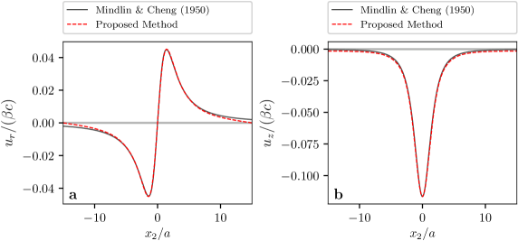
Figure 2: Normalized surface displacements due to a hydrostatic spherical inclusion in a half-space. Comparison between the Mindlin and Cheng [1950] solution and the proposed VIM.The displacements are shown along the $x_{1}=x_{3}=0$ line. The agreement between the analytical and computed solutions is very good in the central part of the periodicity cell, while distortion induced by periodic conditions becomes apparent near its boundary.

Recalling now that ${\boldsymbol{\sigma}}={{\boldsymbol{\mathcal{C}}}}:{\boldsymbol{\nabla}}\mathcal{N}[{\boldsymbol{w}}]-{\boldsymbol{w}}$, Fig. 3 shows the validation of ${\boldsymbol{\nabla}}\mathcal{N}$ by way of a comparison of stresses $\sigma_{\theta}$, and $\sigma_{z}$ produced by the inclusion, whose values along the vertical line $r=0$ going through the inclusion center are shown in Figs. 3a and 3b, respectively. The relevant analytical values are (for $r=0$):

$$\sigma_{\theta} =\frac{2\mu\beta a^{3}}{3}\Big{(}\frac{4\nu-3}{{(z+c)}^{3}}+\frac{6c}{{(z+c)}^{4}}+\frac{1}{{|z-c|}^{3}}\Big{)} \sigma_{z} =\frac{2\mu\beta a^{3}}{3}\Big{(}\frac{6z+c}{{(z+c)}^{4}}-\frac{2}{|z-c|^{3}}\Big{)} z\in[0,a[\cup]3a,+\infty[,$$ (67)

$$\sigma_{\theta} =\frac{2\mu\beta a^{3}}{3}\Big{(}\frac{4\nu-3}{{(z+c)}^{3}}+\frac{6c}{{(z+c)}^{4}}-\frac{2}{a^{3}}\Big{)}, \sigma_{z} =\frac{2\mu\beta a^{3}}{3}\Big{(}\frac{6z+c}{{(z+c)}^{4}}-\frac{2}{a^{3}}\Big{)}, z\in]a,3a[$$ (68)

with $\beta=\alpha T\frac{1+\nu}{1-\nu}$. We observe on Figures 3a and 3b a Gibbs effect at the inclusion boundary, caused by the Fourier approximation of the discontinuity of the eigenstrain, as mentioned in Section 3.1. This should however not have a significant effect on elastoplastic simulations, as plastic deformations should be continuous provided there is no shear band. Nonetheless, our method accurately represents the large discontinuity in the tangential stress, see Figure 3b.

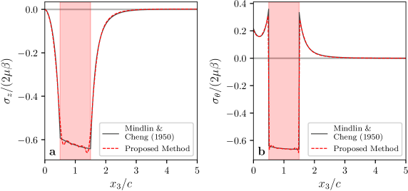
Figure 3: Normalized stresses due to a hydrostatic spherical inclusion in a half-space. Comparison between the Mindlin and Cheng [1950] solution and the proposed volume integral method. The stresses are shown along the $x_{3}$ axis. The red region is where the eigenstrain ${\boldsymbol{\varepsilon}}=\alpha T{{\boldsymbol{I}}}$ is imposed. One can observe a good agreement of the numerical approximation with the analytical solution outside the inclusion. Some Gibbs effect can be observed at the boundary of the inclusion, with spurious oscillations in the inclusion. This is due to the Fourier approximation of the discontinuous eigenstrain function.

6.2 Elastoplastic contact validation

We validate our complete proposed method (including elastoplastic contact) against an axi-symmetric FEM analysis by Hardy et al. [1971] which provides the surface pressure distribution for a rigid spherical indenter on an elastic-perfectly plastic material. For Hertzian contact with $\nu=0.3$, the maximum shear stress occurs at a depth $x_{3}\approx 0.57a$, with $a$ the contact radius. Moreover, the von Mises stress reaches $\sigma_{\text{y}}$ for a maximum surface pressure of $p_{\text{y}}=1.6\sigma_{\text{y}}$ [Johnson, 1985]. From this, one can compute the total load $W_{\text{y}}$ and contact radius $a_{\text{y}}$ at the onset of yield [Hardy et al., 1971]:

$$\text{(a) \ }W_{\text{y}}=\frac{\pi^{3}R^{2}}{6{E^{\star}}^{2}}p_{\text{y}}^{3},\quad\quad\text{(b) \ }a_{\text{y}}=\sqrt{\frac{3W_{\text{y}}}{2\pi p_{\text{y}}}},$$ (69)

where $R$ is the indenter radius and $E^{\star}:=E/(1-\nu^{2})$ is the Hertz elastic modulus. We also define $\tau_{\text{y}}:=\sigma_{\text{y}}/\sqrt{3}$ as the shear yield stress. $W_{\text{y}}$, $a_{\text{y}}$ and $\tau_{\text{y}}$ are used to normalize loads, lengths and stresses respectively. Figure 4 compares the surface pressure $p[{\boldsymbol{u}}]$ computed using Algorithm 1 with the corresponding values obtained by Hardy et al. [1971] (dashed lines), for different load ratios $W/W_{\text{y}}$. The dark continuous line is the circumferential average of the pressure, while the lighter zone shows the maximum and minimum pressure for a given radial coordinate $r$. The difference between the maximum and minimum pressures at the edge of contact is due to the discretization and the periodic boundary conditions, which make the contact region shape deviate from a disk. The simulation parameters are given in C.2. As mentioned in [Hardy et al., 1971], normalized results are independent of the $E/\tau_{\text{y}}$ ratio.

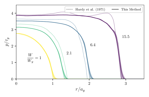
Figure 4: Elastic perfectly-plastic Hertzian contact, comparison with Hardy et al. [1971]. Increase of the applied load beyond the initial yield shows that the pressure profile deviates from the elliptic Hertzian profile by flattening of the curve at the axis of symmetry, with a plateau whose extent increases with the load. The results of Hardy et al. [1971] however show oscillations of the pressure profile at high plastic loads which is not reproduced by our simulation. As there is, to our knowledge, no physical reason to these oscillations, they are likely due to the coarse discretization of the finite-element mesh they used in their study. The simulation parameters are given in C.2

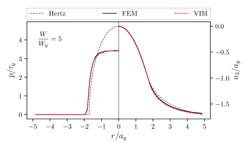
Figure 5: Elastoplastic Hertzian contact. Comparison between the elastic Hertz solution [Johnson, 1985], a simulation using algorithm 1 where the surface residual displacement is calculated by FEM, and a full VIM simulation. Both simulations have identical surface discretization. As expected [Johnson, 1968], the plastic pressure distribution deviates from the elliptical shape of the Hertzian distribution. The contact radius is larger in the plastic case. The simulation parameters are given in C.3.

Both solutions show a flattening of the initially-ellipsoidal pressure distribution near the axis of symmetry (also observed in Johnson [1968], Jacq et al. [2002], Wang et al. [2013]), with a plateau that extends as the load is increased. There are however significant differences between the two sets of results: in the plastic range, the agreement on both the contact radius and the plateau value is poor. Also, the results of Hardy et al. [1971] feature oscillations in the pressure profile at the highest loading increment, which are likely due to the coarse mesh that was used, combined with large loading steps .

To assess these effects and confirm the latter remark, we have effected additional comparisons, this time to an implementation of algorithm 1 where the strain increment is computed using a first-order FEM approach with the open-source high-performance code Akantu [Richart and Molinari, 2015], the rest of the algorithm using the same code as for the VIM. The geometry, material properties, loading and discretization are as given in C.3. Figure 5 shows the surface pressure and vertical displacement for a load ratio of $W/W_{\text{y}}=5$, the corresponding Hertz elastic solution being also plotted for additional comparison. We observe an excellent agreement between the FEM and VIM solutions. In addition, Figure 6 shows good qualitative agreement between the values of $|{\boldsymbol{\varepsilon}}^{p}|$ on a symmetry plane obtained for the same load with the FEM and the VIM.

Figure 6: Plastic strain norm $|{\boldsymbol{\varepsilon}}^{p}|$ in elastoplastic Hertzian contact. Results obtained with algorithm 1, with the plastic problem solved using our VIM approach (left) or a first order FEM (right). Note that in the FEM case, plastic deformations are piece-wise constant, whereas in the volume integral result they are interpolated between nodal values (cf. Section 3). Nonetheless, the solutions give similar plastic zone size and maximum plastic deformation norm. The simulation parameters are given in C.3.

7 Algorithmic complexity

We now compare the computational cost of the application of the operator $\mathcal{N}$ to that of an elastic solve step of a finite elements simulation involving the same number $N=N_{1}N_{2}N_{3}$ of nodes. Irrespective of the numerical method used, the optimal complexity would be $\mathcal{O}(N)$. In the proposed methodology, the evaluation of $\mathcal{N}[{\boldsymbol{w}}]$ for given ${\boldsymbol{w}}$ is decomposed into two computational steps: the multiple 2D fast-Fourier transforms and the computation of equation (50). Assuming $N_{1}=N_{2}=N_{3}$, the former has a complexity of $\mathcal{O}(N_{1}N_{2}N_{3}\log(N_{1}N_{2}))\sim\mathcal{O}(N\log(N))$, while the latter has a complexity of $\mathcal{O}(N_{1}N_{2}N_{3}^{2})\sim\mathcal{O}(N^{4/3})$ with a naive implementation. Using the cutoff proposed in 3.2 brings the algorithmic complexity of the evaluations of (50) down to $\mathcal{O}(N)$ (see D), so the asymptotic cost of evaluating $\mathcal{N}[{\boldsymbol{w}}]$ is $\mathcal{O}(N\log(N))$. For the direct solve step of a finite element elastic simulation with $N$ nodes, the algorithmic complexitiy of a sparse Cholesky factorization is $\mathcal{O}(N^{3/2})$ [Lipton et al., 1979]. We compare in figure 7 the relative computation times of the application of $\mathcal{N}$ and the elastic solve step of Akantu, which uses the direct solver package MUMPS [Amestoy et al., 2001] to perform the factorization. A regular mesh with $N$ nodes was used. We can observe that for large problem sizes the computation times fit the theoretical asymptotic complexities, showing the clear advantage of the proposed VIM over FEM. One should also note that memory needed for the factorization of the stiffness matrix for $2^{21}$ nodes was larger than 128 GB whereas the VIM only required 1.27 GB for this case. For large problems, both the memory imprint and (absolute) computing time are two orders of magnitude smaller with the proposed approach.

As a closing remark, evaluating $\mathcal{N}$ in physical space and without any acceleration method would entail a $\mathcal{O}(N^{2})$ complexity, making its use unrealistic for 3D problems. This complexity can be brought down to $\mathcal{O}(N)$ by means of a multi-level fast multipole (ML-FM) approach. However, implementing the latter is quite involved in general, and here would require intricate and expensive close-range numerical quadrature methods for dealing with the strong singularity and complex expressions of the kernel in the physical space. This may explain why ML-FM treatments of VIMs have received only limited attention to date.

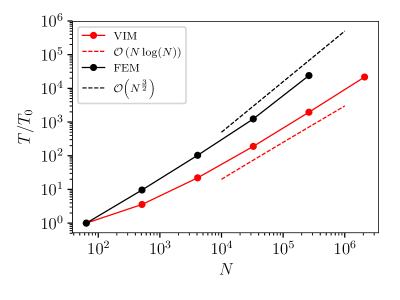
Figure 7: Relative computation times for VIM and FEM. We compare the application of the operator $\mathcal{N}$ to an elastostatic FEM solve step (Cholesky factorization). The reference time $T_{0}$ is $T_{0}=1.41\cdot 10^{-3}$s for the VIM and $T_{0}=1.77\cdot 10^{-2}$s for the FEM. The scaling for large problem sizes agrees with the theoretical algorithmic complexities. For $N=2^{21}$ the stiffness matrix factorization needed over 128 GB of memory, an amount two orders of magnitude larger than what is required for the VIM.

8 Rough surface contact

We now showcase the applicability of the method to rough surface contact. Self-affine surfaces are commonly used in this context [Yastrebov et al., 2012, Müser et al., 2017]. They are characterized by a power-spectral density obeying a power law [Persson et al., 2005]. For this simulation, we generate a random rough surface using an FFT filter algorithm [Hu and Tonder, 1992], specifying a Hurst exponent of 0.8, with the largest wavelength $\lambda_{l}$, the roll-off wavelength $\lambda_{r}$ and the smallest wavelength $\lambda_{s}$ given by $L/\lambda_{l}=1$, $\lambda_{l}/\lambda_{r}=2$ and $\lambda_{s}/\Delta l=4$ (cf. C.5 for graphical representation of the PSD) where $L:=L_{1}=L_{2}$ and $\Delta l=L/N$ (equal number of points $N=512$ in $x_{1}$ and $x_{2}$). The $x_{3}$ domain $L_{3}=0.4\cdot L$ is discretized in $N_{3}=64$ points, yielding upwards of 100 million degrees of freedom for the plasticity problem (where $\Delta{\boldsymbol{\varepsilon}}$ is the primary unknown) solved on a single compute node. The Poisson coefficient is set to $\nu=0.3$, the yield ratio to $\sigma_{\text{\scriptsize y}}/E=10^{-1}$ and the hardening modulus to $E_{\text{\scriptsize h}}=10^{-2}E$.

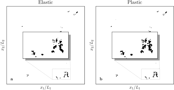
Figure 8: Contact area comparison in rough surface contact. Both simulations have the same contacting rough surface. Figure a shows the elastic contact area, with the inset zooming on the lower left cluster of micro-contacts. Figure b shows the contact area obtained for the same load in the case of elastic-plastic contact, which is 24% larger than in the elastic case. The details of the micro-contacts are also different: disjoint elastic contacts have coalesced in the plastic case, and some new contacts have appeared. This may change the micro-contact distribution, influencing phenomena such as wear.

Figure 8 shows a comparison between the actual contact areas produced by elastic and elastoplastic contact simulations with the same applied load $W=10^{-3}E\sqrt{\langle|\nabla h|^{2}\rangle}$ (normalization by the root-mean-square of slopes collapses the load to contact area relation in the elastic case, see Hyun et al., 2004). It should be mentioned that algorithm 1 is not particularly well suited for rough surface contact: it is by default not robust to large load steps and requires tuning of the relaxation parameter, which renders the convergence slow and very dependent on discretization and on $\sigma_{\text{\scriptsize y}}/E$. The lack of robustness of the algorithm prevents full use of the capacities of Newton-Krylov and spectral residual solvers, which usually allow for large load steps. To our knowledge, this has not yet been addressed, as recent work on elastic-plastic contact with VIMs also use alternating projection approach of algorithm 1 [Amuzuga et al., 2016, Zhang et al., 2018]. Finding a coupling algorithm better suited than algorithm 1 to rough surface contact will be part of our future work on the subject. For instance, the elastoplastic contact problem considered here could be recast as a second-order conic program. This suggests the possibility of resorting to interior point methods, which have proved robust and efficient in other contexts also involving large-scale simulations for non-linear materials [Bleyer, 2018].

Hence, we have confined this preliminary study to small contact areas and a rather large $\sigma_{\text{\scriptsize y}}/E$ ratio (which would correspond to the behavior of elastomers). Noticeable differences are nonetheless observed between the elastic and elastic-plastic solutions: with plasticity, the contact area is 24% larger (for the same load) and details of micro-contacts are qualitatively different. The insets of figure 8 show that some micro-contacts coalesce due to plasticity while others grow larger. This may have implications on the distribution of micro-contact areas, which plays a crucial role in wear [Frérot et al., 2018].

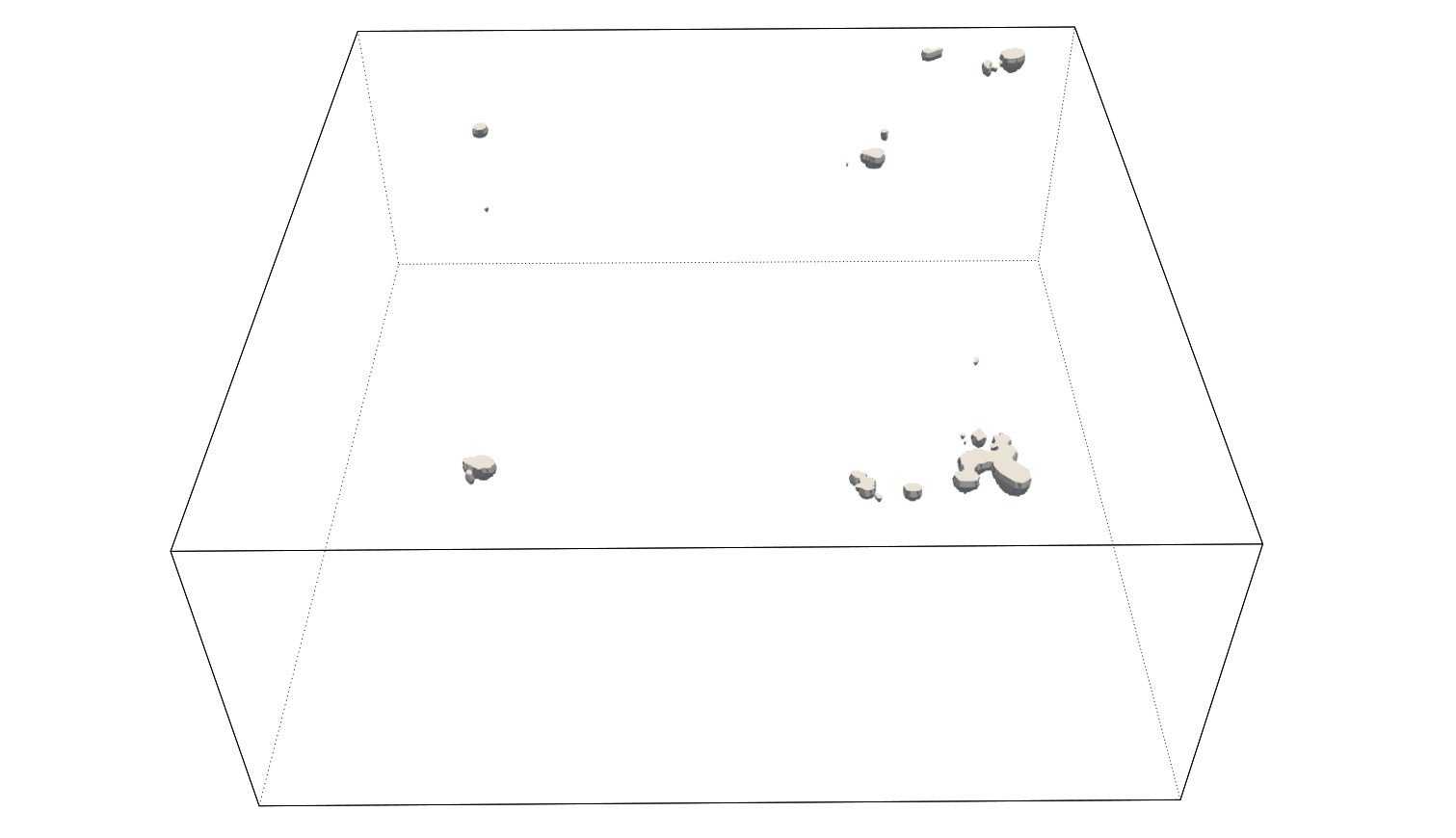
Figure 9: Plastic volumes in material bulk. As expected, they are located beneath contact zones (see figure 8). Even for low contact area situations, the plastic activity reaches the contact surface.

Figure 9 shows the plastic volumes in the bulk of the material. Even for such a small contact area, plastic activity in the subsurface material is enough to make disjoint micro-contacts share the same plastic deformation zones. As the proposed method allows an unprecedentedly fine representation of the plastic deformations, one can exploit this data to compute statistics on the distribution of plastic volumes.

9 Conclusion

We have developed a new, high-efficiency spectral method for solving elastoplastic contact problems. It relies on a novel derivation of the Mindlin fundamental solution directly in the 2D partial Fourier coordinate space, allowing memory savings, error reduction and acceleration of the remaining one-dimensional convolution in a periodic setting, while exploiting the performance of the fast-Fourier transform. We also show the mathematical soundness of the different steps in the method (with the theory of distributions), justifying the discretization of the integral operators which was simply assumed in previous works on spectral methods in contact.

The performance of the method comes from the periodic nature of the problem and its intimate relationship with the discrete Fourier transform. In the investigation of physical phenomena, having a periodic system is not a problem as long as surfaces are representative, i.e. their largest wavelength is several times smaller than the size of the system [Yastrebov et al., 2012]. This entails a large number of points in the discretized system, which our method is capable of handling while still considering the non-linear and volumetric nature of plastic deformations. The latter can be resolved with an accuracy fine enough for computation and statistics of plastic volumes, which have until now never been studied in detail. As comparison, a simulation of 100 million degrees of freedom with a finite-element approach would require distributing the computational load over several cluster nodes, whereas we have shown that our approach can handle such a simulation on a single node (both the required memory and computing time being two orders of magnitude smaller). The performance of the global elastoplastic contact solver is currently the bottleneck of the presented method and renders a systematic study of rough surface contact difficult. Our next efforts will be to replace the solver by an interior-point method, which have proven efficient in a similar class of problems [Bleyer, 2018].

As mentioned by Vakis et al. [2018] and Müser et al. [2017], there are many tribological phenomena that will benefit from accurate results of elastic-plastic rough contact for which this method can be instrumental.

Appendix A Invertibility and linear independence of ${\boldsymbol{A}}^{+}$ and ${\boldsymbol{A}}^{-}$

Due to its structure, ${\boldsymbol{A}}^{\pm}$ has two unit eigenvalues. The determinant of ${\boldsymbol{A}}^{\pm}$ is therefore:

$$\det({\boldsymbol{A}}^{\pm})=\text{trace}({\boldsymbol{A}}^{\pm}) =e^{\mp qy_{3}}\left(\frac{c}{c+2}qy_{3}({\boldsymbol{\Delta}}^{\pm}\cdot{\boldsymbol{\Delta}}^{\pm})+1\right)$$ (70)

$$=e^{\mp qy_{3}}\left(\frac{c}{c+2}qy_{3}\left(1-{\left(\frac{q_{1}}{q}\right)}^{2}-{\left(\frac{q_{2}}{q}\right)}^{2}\right)+1\right)=e^{\mp qy_{3}},$$ (71)

so does not vanish $\forall({\boldsymbol{q}},y_{3})\in\mathbb{R}^{2}\times\mathbb{R}$. Therefore ${\boldsymbol{A}}^{\pm}$ is invertible and $\mathrm{rank}({\boldsymbol{A}}^{\pm})=3$. The linear independence of ${\boldsymbol{A}}^{+}$ and ${\boldsymbol{A}}^{-}$ then stems from their being proportional to different exponential functions.

Appendix B Proof of Theorem 2

The displacement ${\boldsymbol{u}}=\mathcal{N}[{\boldsymbol{w}}]$ ($\mathcal{N}$ being the Mindlin integral operator) solves the problem

$$\text{(a) \ }{{\boldsymbol{\mathrm{N}}}}[{\boldsymbol{u}}]=-\text{div}{\boldsymbol{w}}\quad\text{in }{\mathcal{B}},\qquad\text{(b) \ }{\boldsymbol{T}}[{\boldsymbol{u}}]={\boldsymbol{0}}\quad\text{on }\partial{\mathcal{B}}$$ (72)

In the non-periodic case, the partial Fourier version of the above problem is the ODE system

$$\text{(a) \ }{{\widehat{\boldsymbol{\mathrm{N}}}}}({\boldsymbol{q}})\cdot{\widehat{\boldsymbol{u}}}({\boldsymbol{q}},y_{3})=-{\widehat{\boldsymbol{\nabla}}}\cdot{\widehat{\boldsymbol{w}}}({\boldsymbol{q}},y_{3})\quad\big{(}y_{3}\in[0,\infty[\big{)},\qquad\qquad\text{(b) \ }{\widehat{\boldsymbol{T}}}({\boldsymbol{q}})\cdot{\widehat{\boldsymbol{u}}}({\boldsymbol{q}},x_{3})={\boldsymbol{0}},$$ (73)

where ${\boldsymbol{q}}\in\mathbb{R}^{2}$ acts as a parameter. Solving (73) for arbitrary sources ${\widehat{\boldsymbol{w}}}({\boldsymbol{q}},y_{3})$ yields ${\widehat{\boldsymbol{u}}}({\boldsymbol{q}},\raisebox{0.5pt}{\scalebox{0.6}{$\bullet$}})=\widehat{\mathcal{N}[{\boldsymbol{w}}]}({\boldsymbol{q}},\raisebox{0.5pt}{\scalebox{0.6}{$\bullet$}})$ for any ${\boldsymbol{q}}\in\mathbb{R}^{2}$, $\widehat{\mathcal{N}[{\boldsymbol{w}}]}$ being given by (15) with ${\widehat{\boldsymbol{H}}}={\widehat{\boldsymbol{\nabla G}}}$.

Consider now the case where ${\boldsymbol{w}}$ is $\mathcal{B}_{p}$-periodic, so has the Fourier series form (45a). Since $\mathcal{F}[\exp(\mathrm{i}{\boldsymbol{a}}\cdot\tilde{\boldsymbol{x}}{})]=\delta({\boldsymbol{q}}-{\boldsymbol{a}})$ for $\mathcal{F}[\raisebox{0.5pt}{\scalebox{0.6}{$\bullet$}}]$ as defined by (13), this implies

$${\widehat{\boldsymbol{w}}}({\boldsymbol{q}},y_{3})=\sum_{{\boldsymbol{k}}\in\mathbb{Z}^{2}}{\widehat{\boldsymbol{\mathrm{w}}}}({\boldsymbol{k}},x_{3})\delta({\boldsymbol{q}}-2\pi\bar{{\boldsymbol{k}}}).$$ (74)

Using this in the right-hand side of (73a), we deduce that ${\widehat{\boldsymbol{u}}}$ must also assume the form of a series of weighted Dirac distributions with the same supports. Hence ${\boldsymbol{u}}$ is also $\mathcal{B}_{p}$-periodic and can be expressed as a Fourier series (45b) with its coefficients ${\widehat{\boldsymbol{\mathrm{u}}}}({\boldsymbol{k}},x_{3})$ to be determined:

$${\widehat{\boldsymbol{u}}}({\boldsymbol{q}},y_{3})=\sum_{{\boldsymbol{k}}\in\mathbb{Z}^{2}}{\widehat{\boldsymbol{\mathrm{u}}}}({\boldsymbol{k}},x_{3})\delta({\boldsymbol{q}}-2\pi\bar{{\boldsymbol{k}}}).$$ (75)

Applying the partial Fourier transform to problem (72) and inserting ${\widehat{\boldsymbol{w}}}({\boldsymbol{q}},y_{3})$, ${\widehat{\boldsymbol{u}}}({\boldsymbol{q}},y_{3})$ as given above thus yields

$${{\widehat{\boldsymbol{\mathrm{N}}}}}({\boldsymbol{q}})\cdot\sum_{{\boldsymbol{k}}\in\mathbb{Z}^{2}}{\widehat{\boldsymbol{\mathrm{u}}}}({\boldsymbol{k}},x_{3})\delta({\boldsymbol{q}}-2\pi\bar{{\boldsymbol{k}}}) =-\sum_{{\boldsymbol{k}}\in\mathbb{Z}^{2}}{\widehat{\boldsymbol{\nabla}}}\cdot{\widehat{\boldsymbol{\mathrm{w}}}}({\boldsymbol{k}},x_{3})\delta({\boldsymbol{q}}-2\pi\bar{{\boldsymbol{k}}})\qquad y_{3}\in[0,\infty[,$$ (76)

$${\widehat{\boldsymbol{T}}}({\boldsymbol{q}})\cdot\sum_{{\boldsymbol{k}}\in\mathbb{Z}^{2}}{\widehat{\boldsymbol{\mathrm{u}}}}({\boldsymbol{k}},x_{3})\delta({\boldsymbol{q}}-2\pi\bar{{\boldsymbol{k}}}) ={\boldsymbol{0}}.$$ (77)

Using (for example) the distributional equality ${{\widehat{\boldsymbol{\mathrm{N}}}}}({\boldsymbol{q}})\delta({\boldsymbol{q}}-{\boldsymbol{a}})={{\widehat{\boldsymbol{\mathrm{N}}}}}({\boldsymbol{a}})\delta({\boldsymbol{q}}-{\boldsymbol{a}})$, we deduce the relations

$$\text{(a) \ }{{\widehat{\boldsymbol{\mathrm{N}}}}}(2\pi\bar{{\boldsymbol{k}}})\cdot{\widehat{\boldsymbol{u}}}({\boldsymbol{k}},y_{3})=-{\widehat{\boldsymbol{\nabla}}}\cdot{\widehat{\boldsymbol{\mathrm{w}}}}({\boldsymbol{k}},x_{3})\quad y_{3}\in[0,\infty[,\qquad\text{(b) \ }{\widehat{\boldsymbol{T}}}(2\pi\bar{{\boldsymbol{k}}})\cdot{\widehat{\boldsymbol{\mathrm{u}}}}({\boldsymbol{k}},x_{3})={\boldsymbol{0}},\qquad\qquad{\boldsymbol{k}}\in\mathbb{Z}^{2}$$ (78)

which are formally identical to (73) with the replacements ${\boldsymbol{q}}\to 2\pi\bar{{\boldsymbol{k}}}$, ${\widehat{\boldsymbol{u}}}({\boldsymbol{q}},y_{3})\to{\widehat{\boldsymbol{\mathrm{u}}}}({\boldsymbol{k}},x_{3})$ and ${\widehat{\boldsymbol{w}}}({\boldsymbol{q}},y_{3})\to{\widehat{\boldsymbol{\mathrm{w}}}}({\boldsymbol{k}},x_{3})$. This shows that ${\widehat{\boldsymbol{\mathrm{u}}}}({\boldsymbol{k}},\raisebox{0.5pt}{\scalebox{0.6}{$\bullet$}})=\widehat{\mathcal{N}[{\boldsymbol{w}}]}(2\pi\bar{{\boldsymbol{k}}},\raisebox{0.5pt}{\scalebox{0.6}{$\bullet$}})$, where $\widehat{\mathcal{N}[{\boldsymbol{w}}]}$ is still given by (15) with ${\widehat{\boldsymbol{H}}}={\widehat{\boldsymbol{\nabla G}}}$. This completes the proof of the theorem.

Appendix C Simulation data

In this appendix, we give the detailed geometry, discretization and loading of each simulation. We note ${[a,b]}_{n}$ the $[a,b]$ interval discretized in $n$ equally spaced values (including $a$ and $b$).

C.1 Comparison with Mindlin and Cheng [1950]

With $a$ the radius of the inclusion, the free parameters are fixed to:

• Inclusion center $x_{3}$ coordinate $c=2a$

• System size ${[0,15c]}^{2}\times[0,5c]$

• Discretization ${\boldsymbol{N}}=(128,128,126)$.

• $\nu=0.3$

Values of $E$, $\alpha$ or $T$ do not influence the normalized results.

C.2 Comparison with Hardy et al. [1971]

With $R$ the radius of the indenter, the free parameters are fixed to:

• System size ${[0,\frac{20}{3}R]}^{2}\times[0,\frac{10}{3}R]$

• Discretization ${\boldsymbol{N}}=(81,81,32)$

• $\nu=0.3$

• Loading $W/W_{\text{\scriptsize y}}\in{[0.9,15.5]}_{20}\cup\{1,2.1,6.4,15.5\}$ (sorted for monotonic loading history)

Values of $E$ or $\sigma_{\text{\scriptsize y}}$ do not influence the normalized results. The tolerance of algorithm 1 is set to $10^{-9}$.

C.3 Comparison with Akantu [Richart and Molinari, 2015]

With $R$ the radius of the indenter, the free parameters are fixed to:

• System size ${[0,\frac{20}{3}R]}^{2}\times[0,\frac{10}{3}R]$

• Discretization ${\boldsymbol{N}}=(81,81,32)$

• FEM discretization: 81$\times$81 surface nodes, 54 nodes in the $x_{3}$ direction, 85975 total nodes and 460246 linear tetrahedron elements. The mesh is refined at the contact interface.

• $\nu=0.3$

• Loading: $W/W_{\text{\scriptsize y}}\in{[0.7,5]}_{20}$

The tolerance of algorithm 1 is set to $10^{-9}$. The source code of Akantu is available on https://akantu.ch. The finite-element mesh is generated with GMSH [Geuzaine and Remacle, 2009] and results are visualized with Paraview [Ayachit, 2015].

C.4 Scaling simulations

With a cubic domain of side $L=1$, the number of points in the discretized system direction (with $N_{1}=N_{2}=N_{3}$) in both FEM and VIM simulations vary in $\{4^{3},8^{3},16^{3},32^{3},64^{3},128^{3}\}$. The source code for the finite elements simulation can be found here: https://doi.org/10.5281/zenodo.2613614 [Frérot, 2019].

C.5 Rough surface simulation

With $L$ the horizontal system size, the free parameters are fixed to:

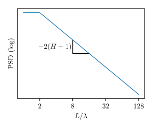
Figure 1: Schematic of power spectrum density for the self-affine rough surface used in Section 8.

• System size ${[0,L]}^{2}\times[0,\frac{2L}{5}]$

• Surface parameters (cf. figure 1):

  • $L/\lambda_{l}=1$

  • $\lambda_{l}/\lambda_{r}=2$

  • $\lambda_{r}/\lambda_{s}=64$

  • $\lambda_{s}/\Delta l=4$

  • $H=0.8$

• Discretization ${\boldsymbol{N}}=(512,512,64)$.

• Loading $W=10^{-3}E\sqrt{\langle|\nabla h|^{2}\rangle}$ (where $\sqrt{\langle|\nabla h|^{2}\rangle}$ is the root-mean-square of slopes).

The tolerance of algorithm 1 is set to $10^{-7}$. The relaxation parameter is set to $\lambda=0.3$.

Appendix D Complexity of integration with cutoff

The cutoff condition on the integration of an element of center $x_{c}^{i}$ for a point of interest $x$ is that $q|x_{c}^{i}-x_{3}|<\varepsilon_{\text{co}}\Leftrightarrow|x_{c}^{i}-x_{3}|<\varepsilon_{\text{co}}/\sqrt{q_{1}^{2}+q_{2}^{2}}$. So for a given value of $x_{3}$, the number of operations needed for the computation of integral (50) for all discrete values of ${\boldsymbol{q}}$ is of the order of:

$$\sum_{{\boldsymbol{k}}\in\mathbb{Z}^{2}_{\boldsymbol{N}}}{\frac{N_{3}}{\sqrt{k_{1}^{2}+k_{2}^{2}}}}.$$ (79)

Since the cutoff is smaller at high wavenumbers the number of terms to be accounted for decreases. We can approximate this series with an integral, which gives the value $N_{3}\sqrt{N_{1}^{2}+N_{2}^{2}}$. Setting $N_{1}=N_{2}=N_{3}$ gives an asymptotic complexity of $\mathcal{O}(N_{3}^{2}\sqrt{N_{1}^{2}+N_{2}^{2}})\sim\mathcal{O}(N)$.

References

- Almqvist et al. [2011] Almqvist, A., Campañá, C., Prodanov, N., Persson, B.N.J., 2011. Interfacial separation between elastic solids with randomly rough surfaces: Comparison between theory and numerical techniques. Journal of the Mechanics and Physics of Solids 59, 2355–2369. doi:10.1016/j.jmps.2011.08.004.
- Amba-Rao [1969] Amba-Rao, C.L., 1969. Fourier transform methods in elasticity problems and an application. Journal of the Franklin Institute 287, 241–249. doi:10.1016/0016-0032(69)90100-8.
- Amestoy et al. [2001] Amestoy, P., Duff, I., L’Excellent, J., Koster, J., 2001. A Fully Asynchronous Multifrontal Solver Using Distributed Dynamic Scheduling. SIAM Journal on Matrix Analysis and Applications 23, 15–41. doi:10.1137/S0895479899358194.
- Amuzuga et al. [2016] Amuzuga, K.V., Chaise, T., Duval, A., Nelias, D., 2016. Fully Coupled Resolution of Heterogeneous Elastic–Plastic Contact Problem. Journal of Tribology 138, 021403. doi:10.1115/1.4032072.
- Archard [1953] Archard, J.F., 1953. Contact and Rubbing of Flat Surfaces. Journal of Applied Physics 24, 981–988. doi:10.1063/1.1721448.
- Ayachit [2015] Ayachit, U., 2015. The ParaView Guide: Updated for ParaView Version 4.3. Full color version ed., Kitware, Los Alamos. OCLC: 944221263.
- Birgin et al. [2014] Birgin, E.G., Martínez, J.M., Raydan, M., 2014. Spectral Projected Gradient Methods: Review and Perspectives. Journal of Statistical Software 60. doi:10.18637/jss.v060.i03.
- Bleyer [2018] Bleyer, J., 2018. Advances in the simulation of viscoplastic fluid flows using interior-point methods. Computer Methods in Applied Mechanics and Engineering 330, 368–394. doi:10.1016/j.cma.2017.11.006.
- Bonnet [1995] Bonnet, M., 1995. Boundary Integral Equation Methods for Solids and Fluids. J. Wiley, Chichester ; New York. OCLC: ocm41368652.
- Bonnet [2017] Bonnet, M., 2017. A modified volume integral equation for anisotropic elastic or conducting inhomogeneities: Unconditional solvability by Neumann series. Journal of Integral Equations and Applications 29, 271–295. doi:10.1216/JIE-2017-29-2-271.
- Bonnet and Mukherjee [1996] Bonnet, M., Mukherjee, S., 1996. Implicit BEM formulations for usual and sensitivity problems in elasto-plasticity using the consistent tangent operator concept. International Journal of Solids and Structures 33, 4461–4480. doi:10.1016/0020-7683(95)00279-0.
- Bowden and Tabor [1939] Bowden, F.P., Tabor, D., 1939. The Area of Contact between Stationary and between Moving Surfaces. Proceedings of the Royal Society of London. Series A, Mathematical and Physical Sciences 169, 391–413.
- Boyd [2001] Boyd, J.P., 2001. Chebyshev and Fourier Spectral Methods. 2nd ed., rev ed., Dover Publications, Mineola, N.Y.
- Bui [1978] Bui, H.D., 1978. Some remarks about the formulation of three-dimensional thermoelastoplastic problems by integral equations. International Journal of Solids and Structures 14, 935–939. doi:10.1016/0020-7683(78)90069-0.
- Bush et al. [1979] Bush, A.W., Gibson, R.D., Keogh, G.P., 1979. Strongly Anisotropic Rough Surfaces. Journal of Lubrication Technology 101, 15–20. doi:10.1115/1.3453271.
- Bush et al. [1975] Bush, A.W., Gibson, R.D., Thomas, T.R., 1975. The elastic contact of a rough surface. Wear 35, 87–111. doi:10.1016/0043-1648(75)90145-3.
- Campañá and Müser [2006] Campañá, C., Müser, M.H., 2006. Practical Green’s function approach to the simulation of elastic semi-infinite solids. Physical Review B 74, 075420. doi:10.1103/PhysRevB.74.075420.
- Campañá and Müser [2007] Campañá, C., Müser, M.H., 2007. Contact mechanics of real vs. randomly rough surfaces: A Green’s function molecular dynamics study. EPL (Europhysics Letters) 77, 38005. doi:10.1209/0295-5075/77/38005.
- Campañá et al. [2008] Campañá, C., Müser, M.H., Robbins, M.O., 2008. Elastic contact between self-affine surfaces: Comparison of numerical stress and contact correlation functions with analytic predictions. Journal of Physics: Condensed Matter 20, 354013. doi:10.1088/0953-8984/20/35/354013.
- Carbone et al. [2009] Carbone, G., Scaraggi, M., Tartaglino, U., 2009. Adhesive contact of rough surfaces: Comparison between numerical calculations and analytical theories. The European Physical Journal E 30, 65–74. doi:10.1140/epje/i2009-10508-5.
- Chaillat and Bonnet [2014] Chaillat, S., Bonnet, M., 2014. A new Fast Multipole formulation for the elastodynamic half-space Green’s tensor. Journal of Computational Physics 258, 787–808. doi:10.1016/j.jcp.2013.11.010.
- Chen et al. [2008] Chen, W.W., Liu, S., Wang, Q.J., 2008. Fast Fourier Transform Based Numerical Methods for Elasto-Plastic Contacts of Nominally Flat Surfaces. Journal of Applied Mechanics 75, 011022. doi:10.1115/1.2755158.
- Cooley and Tukey [1965] Cooley, J.W., Tukey, J.W., 1965. An Algorithm for the Machine Calculation of Complex Fourier Series. Mathematics of Computation 19, 297–301. doi:10.2307/2003354.
- Dautray and Lions [2000] Dautray, R., Lions, J.L., 2000. Mathematical Analysis and Numerical Methods for Science and Technology: Volume 2 Functional and Variational Methods. OCLC: 913437931.
- Duvaut and Lions [1972] Duvaut, G., Lions, J.L., 1972. Les inéquations en mécanique et en physique. Dunod, Paris.
- Firth [1992] Firth, J.M., 1992. Discrete Transforms. 1st ed ed., Chapman & Hall, London ; New York.
- Fredholm [1900] Fredholm, I., 1900. Sur les équations de l’équilibre d’un corps solide élastique. Acta Mathematica 23, 1–42. doi:10.1007/BF02418668.
- Frérot [2018] Frérot, L., 2018. The Mindlin Fundamental Solution - A Fourier Approach. Zenodo. doi:10.5281/zenodo.1492149.
- Frérot [2019] Frérot, L., 2019. Supplementary codes and data to ”A Fourier-accelerated volume integral method for elastoplastic contact”. Zenodo. doi:10.5281/zenodo.2613614.
- Frérot et al. [2018] Frérot, L., Aghababaei, R., Molinari, J.F., 2018. A mechanistic understanding of the wear coefficient: From single to multiple asperities contact. Journal of the Mechanics and Physics of Solids 114, 172–184. doi:10.1016/j.jmps.2018.02.015.
- Frigo and Johnson [2005] Frigo, M., Johnson, S.G., 2005. The Design and Implementation of FFTW3. Proceedings of the IEEE 93, 216–231. doi:10.1109/JPROC.2004.840301.
- Gao and Davies [2000] Gao, X.W., Davies, T.G., 2000. An effective boundary element algorithm for 2D and 3D elastoplastic problems. International Journal of Solids and Structures 37, 4987–5008. doi:10.1016/S0020-7683(99)00188-2.
- Geuzaine and Remacle [2009] Geuzaine, C., Remacle, J.F., 2009. Gmsh: A 3-D finite element mesh generator with built-in pre- and post-processing facilities. International Journal for Numerical Methods in Engineering 79, 1309–1331. doi:10.1002/nme.2579.
- Gintides and Kiriaki [2015] Gintides, D., Kiriaki, K., 2015. Solvability of the integrodifferential equation of Eshelby’s equivalent inclusion method. The Quarterly Journal of Mechanics and Applied Mathematics 68, 85–96. doi:10.1093/qjmam/hbu025.
- Greenwood and Williamson [1966] Greenwood, J.A., Williamson, J.B.P., 1966. Contact of Nominally Flat Surfaces. Proceedings of the Royal Society of London A: Mathematical, Physical and Engineering Sciences 295, 300–319. doi:10.1098/rspa.1966.0242.
- Guiggiani and Gigante [1990] Guiggiani, M., Gigante, A., 1990. A General Algorithm for Multidimensional Cauchy Principal Value Integrals in the Boundary Element Method. Journal of Applied Mechanics 57, 906–915. doi:10.1115/1.2897660.
- Hardy et al. [1971] Hardy, C., Baronet, C.N., Tordion, G.V., 1971. The elasto-plastic indentation of a half-space by a rigid sphere. International Journal for Numerical Methods in Engineering 3, 451–462. doi:10.1002/nme.1620030402.
- Hu and Tonder [1992] Hu, Y., Tonder, K., 1992. Simulation of 3-D random rough surface by 2-D digital filter and fourier analysis. International Journal of Machine Tools and Manufacture 32, 83–90. doi:10.1016/0890-6955(92)90064-N.
- Hyun et al. [2004] Hyun, S., Pei, L., Molinari, J.F., Robbins, M.O., 2004. Finite-element analysis of contact between elastic self-affine surfaces. Physical Review E 70, 026117. doi:10.1103/PhysRevE.70.026117.
- Jacq et al. [2002] Jacq, C., Nélias, D., Lormand, G., Girodin, D., 2002. Development of a Three-Dimensional Semi-Analytical Elastic-Plastic Contact Code. Journal of Tribology 124, 653. doi:10.1115/1.1467920.
- Johnson [1968] Johnson, K.L., 1968. An experimental determination of the contact stresses between plastically deformed cylinders and sphere, in: Engineering Plasticity : Papers for a Conference Held in Cambridge, March 1968, Cambridge : University Press, Cambridge. pp. 341–461.
- Johnson [1985] Johnson, K.L., 1985. Contact Mechanics. Cambridge University Press, Cambridge. doi:10.1017/CBO9781139171731.
- Johnson et al. [1985] Johnson, K.L., Greenwood, J.A., Higginson, J.G., 1985. The contact of elastic regular wavy surfaces. International Journal of Mechanical Sciences 27, 383–396. doi:10.1016/0020-7403(85)90029-3.
- Jones et al. [2001] Jones, E., Oliphant, T., Peterson, P., et al., 2001. SciPy: Open source scientific tools for Python.
- Kalker [1977] Kalker, J.J., 1977. Variational Principles of Contact Elastostatics. IMA Journal of Applied Mathematics 20, 199–219. doi:10.1093/imamat/20.2.199.
- Knoll and Keyes [2004] Knoll, D.A., Keyes, D.E., 2004. Jacobian-free Newton–Krylov methods: A survey of approaches and applications. Journal of Computational Physics 193, 357–397. doi:10.1016/j.jcp.2003.08.010.
- La Cruz et al. [2006] La Cruz, W., Martínez, J., Raydan, M., 2006. Spectral residual method without gradient information for solving large-scale nonlinear systems of equations. Mathematics of Computation 75, 1429–1448. doi:10.1090/S0025-5718-06-01840-0.
- Li and Berger [2003] Li, J., Berger, E.J., 2003. A semi-analytical approach to three-dimensional normal contact problems with friction. Computational Mechanics 30, 310–322. doi:10.1007/s00466-002-0407-y.
- Lipton et al. [1979] Lipton, R., Rose, D., Tarjan, R., 1979. Generalized Nested Dissection. SIAM Journal on Numerical Analysis 16, 346–358. doi:10.1137/0716027.
- Love [1892] Love, A.E.H., 1892. A Treatise on the Mathematical Theory of Elasticity. volume 1. Cambridge University Press, Cambridge, U.K.
- Mindlin [1936] Mindlin, R.D., 1936. Force at a Point in the Interior of a Semi-Infinite Solid. Journal of Applied Physics 7, 195–202. doi:10.1063/1.1745385.
- Mindlin and Cheng [1950] Mindlin, R.D., Cheng, D.H., 1950. Thermoelastic Stress in the Semi-Infinite Solid. Journal of Applied Physics 21, 931–933. doi:10.1063/1.1699786.
- Moulinec and Suquet [1998] Moulinec, H., Suquet, P., 1998. A numerical method for computing the overall response of nonlinear composites with complex microstructure. Computer Methods in Applied Mechanics and Engineering 157, 69–94. doi:10.1016/S0045-7825(97)00218-1.
- Müser and Wang [2018] Müser, M., Wang, A., 2018. Contact-Patch-Size Distribution and Limits of Self-Affinity in Contacts between Randomly Rough Surfaces. Lubricants 6, 85. doi:10.3390/lubricants6040085.
- Müser [2018] Müser, M.H., 2018. Internal, elastic stresses below randomly rough contacts. Journal of the Mechanics and Physics of Solids 119, 73–82. doi:10.1016/j.jmps.2018.06.012.
- Müser et al. [2017] Müser, M.H., Dapp, W.B., Bugnicourt, R., Sainsot, P., Lesaffre, N., Lubrecht, T.A., Persson, B.N.J., Harris, K., Bennett, A., Schulze, K., Rohde, S., Ifju, P., Sawyer, W.G., Angelini, T., Esfahani, H.A., Kadkhodaei, M., Akbarzadeh, S., Wu, J.J., Vorlaufer, G., Vernes, A., Solhjoo, S., Vakis, A.I., Jackson, R.L., Xu, Y., Streator, J., Rostami, A., Dini, D., Medina, S., Carbone, G., Bottiglione, F., Afferrante, L., Monti, J., Pastewka, L., Robbins, M.O., Greenwood, J.A., 2017. Meeting the Contact-Mechanics Challenge. Tribology Letters 65, 118. doi:10.1007/s11249-017-0900-2.
- Pastewka and Robbins [2014] Pastewka, L., Robbins, M.O., 2014. Contact between rough surfaces and a criterion for macroscopic adhesion. Proceedings of the National Academy of Sciences 111, 3298–3303. doi:10.1073/pnas.1320846111.
- Pei et al. [2005] Pei, L., Hyun, S., Molinari, J.F., Robbins, M.O., 2005. Finite element modeling of elasto-plastic contact between rough surfaces. Journal of the Mechanics and Physics of Solids 53, 2385–2409. doi:10.1016/j.jmps.2005.06.008.
- Persson [2006] Persson, B.N.J., 2006. Contact mechanics for randomly rough surfaces. Surface Science Reports 61, 201–227. doi:10.1016/j.surfrep.2006.04.001.
- Persson et al. [2005] Persson, B.N.J., Albohr, O., Tartaglino, U., Volokitin, A.I., Tosatti, E., 2005. On the nature of surface roughness with application to contact mechanics, sealing, rubber friction and adhesion. Journal of Physics: Condensed Matter 17, R1. doi:10.1088/0953-8984/17/1/R01.
- Pohrt and Li [2014] Pohrt, R., Li, Q., 2014. Complete boundary element formulation for normal and tangential contact problems. Physical Mesomechanics 17, 334–340. doi:10.1134/S1029959914040109.
- Polonsky and Keer [1999a] Polonsky, I.A., Keer, L.M., 1999a. A Fast and Accurate Method for Numerical Analysis of Elastic Layered Contacts. Journal of Tribology 122, 30–35. doi:10.1115/1.555323.