Rectification of Spin Current in Inversion-Asymmetric Magnets
with Linearly-Polarized Electromagnetic Waves

Abstract

We theoretically propose a method of rectifying spin current with a linearly-polarized electromagnetic wave in inversion-asymmetric magnetic insulators. To demonstrate the proposal, we consider quantum spin chains as a simple example; these models are mapped to fermion (spinon) models via Jordan-Wigner transformation. Using a nonlinear response theory, we find that a dc spin current is generated by the linearly-polarized waves. The spin current shows rich anisotropic behavior depending on the direction of the electromagnetic wave. This is a manifestation of the rich interplay between spins and the waves; inverse Dzyaloshinskii-Moriya, Zeeman, and magnetostriction couplings lead to different behaviors of the spin current. The resultant spin current is insensitive to the relaxation time of spinons, a property of which potentially benefits a long-distance propagation of the spin current. An estimate of the required electromagnetic wave is given.

Introduction — Manipulation of magnetic states and spin current is a key subject in spintronics Spincurrent2012 . In conductive materials, the charge current is often used for such purposes; magnetic domain walls are moved by spin-transfer effect Berger1984 , and spin Hall effects are used to generate spin current Dyakonov1971 ; Hirsch1999 ; Murakami2003 ; Sinova2004 . The concept of spintronics is also applied to magnetic insulators. They have several advantages over the metallic materials: Magnetic excitations typically have longer life time and no ohmic loss. In these magnets, the electromagnetic wave is a “utility tool”. Recent studies demonstrate that magnetic states and excitations can be controlled by electromagnetic waves. For instance, laser control of magnetizations Kimel2005 ; Stanciu2007 ; Kirilyuk2010 ; Mukai2016 ; Takayoshi2014-1 ; Takayoshi2014-2 , magnetic interactions Mentink2015 , and magnetic textures Mochizuki2010 ; Koshibae2014 ; Sato2016 ; Fujita2017-1 ; Fujita2017-2 ; Ono2017 , spin-wave propagation by focused light Satoh2012 ; Hashimoto2017 , etc. have been extensively studied both experimentally and theoretically. These studies demonstrated that the electromagnetic wave has a high potentiality of controlling the magnetic states and opened a subfield utilizing lights, called opto-spintronics Kirilyuk2010 ; Nemec2018 .

In contrast, the manipulation of the spin current carried by magnetic excitations is limited to ferromagnets; spin pumping with the electromagnetic wave is often used to generate the spin current Kajiwara2010 ; Heinrich2011 ; Ohnuma2014 . On the other hand, other magnetic states (antiferromagnetic, spiral, spin liquid states, etc.) potentially have different advantages over ferromagnets. Therefore, a method for the generation and manipulation of spin current in these materials opens up an interesting possibility for spintronics. For this purpose, the usage of electromagnetic waves is desirable because of the highly precise and ultra-fast control.

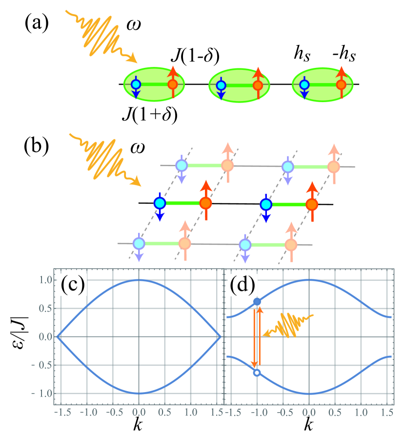
Figure 1: (Color online) Noncentrosymmetric spin chains considered in this work. Schematic picture of (a) a dimerized spin chain and (b) an antiferromagnet of weakly coupled spin chains in a staggered magnetic field. The model consists of two magnetic atoms with different $g$ factor and alternating bonds. Band structure of Jordan-Wigner fermions for (c) $\delta=h_{s}/J=0$, and (d) $\delta=1/3$, and $h_{s}/J=1/10$.

A main issue, however, lies in moving the magnetic excitations using the electromagnetic field; the magnetic excitations do not accelerate/drift by the electromagnetic field because they are chargeless. This problem is potentially solved by utilizing the nonlinear response of magnetic insulators [Fig. 1(a,b)]. In the nonlinear optics of noncentrosymmetric electron systems Sturman1992 ; Tan2016 ; Tokura2018 , a non-trivial dynamics of electrons during the transition process induce a “shift” of the particle position Belinicher1982 ; Sipe2000 ; Morimoto2016 ; Ishizuka2017c . Recent experiments investigating this mechanism find the current propagates faster than the quasi-particle velocity Nakamura2017 ; Ogawa2017 . In addition, it is insensitive to the quasi-particle relaxation time; this is a beneficial property considering the heating by the electromagnetic waves reduces the relaxation time. A spin current with such interesting properties is potentially possible if the shift mechanism of magnetic excitations is generated by the electromagnetic waves.

To investigate the control of spin current by the nonlinear response, we here explore the generation of spin current by the shift mechanism in a quantum spin chain model [Fig. 1(a)]. We show that the spin current is indeed generated by simply applying a linearly-polarized electromagnetic wave if the system possesses one of the three kinds of spin-light couplings: inverse Dzyaloshinskii-Moriya (DM), Zeeman, and magnetostriction couplings. These couplings give rise to rich features in the frequency dependence and anisotropy. Interestingly, the spin current is generated by a different transition process from the electronic photogalvanic effect. The estimate of the magnitude of spin current shows our proposal gives an observable spin current with a reasonable strength of electromagnetic wave.

Noncentrosymmetric spin chains — An $S=1/2$ spin chain with staggered exchange and the magnetic field is used to study the photovoltaic effect of spin current. The Hamiltonian reads

$$H= \sum_{i}J(1+(-1)^{i}\delta)(S_{i}^{x}S_{i+1}^{x}+S_{i}^{y}S_{i+1}^{y})$$

$$\qquad-\sum_{i}(h+(-1)^{i}h_{s})S_{i}^{z}.$$ (1)

Here, $S_{i}^{x,y,z}$ are $S=1/2$ spin operators on site $i$, $J$ is the exchange coupling whose energy scale is usually in gigahertz (GHz) or terahertz (THz) regime, $h$ is the uniform magnetic field along $z$ axis, and $h_{s}$ is the staggered magnetic field. This model has a wide range of applications. An obvious application is to the one-dimensional (1D) dimerized XY spin chains with two alternating ions [Fig. 1(a)]. In this case, the staggered magnetic field $h_{s}$ appears as a consequence of different $g$ factors for the odd- and even-site spins Dender1997 ; Affleck1999 ; Oshikawa1999 ; Feyerherm2000 ; Morisaki2007 ; Umegaki2009 . The model can also be viewed as the effective model for a Néel ordered Ising-like spin chain Shiba1980 ; Coldea2010 ; Faure2018 at zero temperature $T=0$ under a staggered magnetic field, in which the Ising interaction $J_{z}S_{i}^{z}S_{i+1}^{z}$ is treated via the mean-field approximation $S_{i}^{z}=\langle S_{i}\rangle+(S_{i}^{z}-\langle S_{i}\rangle)$. For the Néel ordered state, the field $(-1)^{i}h_{s}$ is the sum of the external staggered field and the mean field $J_{z}\langle S_{i}\rangle=(-1)^{i}J_{z}M_{s}$ ($M_{s}$ is the staggered magnetization). Furthermore, Eq. (1) can also be applied to three-dimensional antiferromagnets of weakly coupled spin chains under a staggered field [Fig. 1(b)]. Treating the inter-chain coupling by a mean-field theory Scalapino1975 ; Schulz1996 ; Sato2004 ; Okunishi2007 gives an effective one-dimensional (1D) model, Eq. (1). Namely, in this system, the staggered field $h_{s}$ is renormalized by the inter-chain Néel order. Note that the dimerization parameter $\delta$ and the staggered field $h_{s}$ break site-center and bond-center inversion symmetries, respectively. Such a noncentrosymmetric nature is necessary for a photogalvanic effect.

The spin model in Eq. (1) is mapped to a fermion model using Jordan-Wigner (JW) transformation Giamarchi2004 ; Gogolin2004 ; Tsvelik2007 . By introducing fermion operators $c_{i}\equiv e^{-i\pi\sum_{j=1}^{i-1}S_{j}^{+}S_{j}^{-}}S_{i}^{-}$ and $c_{i}^{\dagger}\equiv S_{i}^{+}e^{i\pi\sum_{j=1}^{i-1}S_{j}^{+}S_{j}^{-}}$, Eq. (1) is fermionized as

$$H=\sum_{i} \frac{J(1+(-1)^{i}\delta)}{2}\left(c_{i+1}^{\dagger}c_{i}+c_{i}^{\dagger}c_{i+1}\right)$$

$$+(h+(-1)^{i}h_{s})n_{i}.$$ (2)

Here, $S^{\pm}_{i}\equiv S_{i}^{x}\pm iS_{i}^{y}$ are the ladder operators and $n_{i}\equiv c_{i}^{\dagger}c_{i}$ is the number operator for the fermions at $i$th site. Figures 1(c) and 1(d) show the band structure of the JW fermions. The model has a band gap $\Delta_{\frac{\pi}{2}}\equiv 2\sqrt{J^{2}\delta^{2}+h_{s}^{2}}$ for $|\delta|<1$ [Fig. 1(d)], while the gap is $\Delta_{0}\equiv 2\sqrt{J^{2}+h_{s}^{2}}$ if $|\delta|>1$. The model is gapless only if $h_{s}=\delta=0$ [Fig. 1(c)]. Therefore, the ground state is robust against $h$ as long as $h<\Delta/2$, where $\Delta\equiv\min(\Delta_{0},\Delta_{\frac{\pi}{2}})$. We focus on the weak $h$ region of this model in the rest of this work.

The spin current operator for $S^{z}$ is defined from the continuity equation. The current density operator reads

$$J_{sc} \equiv\frac{1}{L}\sum_{i}J(1+(-1)^{i}\delta)(S_{i+1}^{x}S_{i}^{y}-S_{i+1}^{y}S_{i}^{x}),$$ (3)

where $L$ is the number of sites; here, we set the Planck constant $\hbar=1$.

Inverse DM coupling — External electromagnetic waves couple to spins in several different forms. First, we consider the coupling of the electric field to the electric dipole induced by the inverse DM mechanism Katsura2005 ; Takahashi2012 ; Huvonen2009 ; Furukawa2010 ; Tokura2014 :

$$H_{\text{iDM}}= E_{y}(t)\sum_{i}(p+(-1)^{i}p_{s})\left(\bm{S}_{i}\times\bm{S}_{i+1}\right)^{z}.$$ (4)

Here, the chain is along the $x$ axis, $p\mp p_{s}$ is the coefficient for the ferroelectric polarization of odd and even bonds, and $E_{y}(t)=E_{y}\cos(\omega t)$ is the oscillating electric field along the $y$ axis with frequency $\omega$ (typically, GHz or THz). Note that at a special point $p_{s}/p=\delta$, the term $H_{\text{iDM}}$ is analogous to the linear-order coupling of the electrons to the vector potential. We will comment on this case later.

The spin current conductivity is calculated using a quadratic response formula similar to that for photovoltaic effects Kraut1979 . The formula reads

$$\sigma^{(2)}(\omega)=\sum_{\alpha,\beta,\gamma}\int\frac{dk}{2\pi}\frac{[f_{\alpha}(k)-f_{\beta}(k)]B_{\alpha\beta}(k)}{\omega-\varepsilon_{\beta}(k)+\varepsilon_{\alpha}(k)-i/(2\tau)}$$

$$\times\left[\frac{B_{\beta\gamma}(k)J_{\gamma\alpha}(k)}{\varepsilon_{\alpha}(k)-\varepsilon_{\gamma}(k)-i/(2\tau)}-\frac{J_{\beta\gamma}(k)B_{\gamma\alpha}(k)}{\varepsilon_{\gamma}(k)-\varepsilon_{\beta}(k)-i/(2\tau)}\right],$$ (5)

where $\varepsilon_{\alpha}(k)$ is the eigenenergy of an $\alpha$th-band state with momentum $k$ ($\left|\alpha k\right>$), $f_{\alpha}(k)\equiv(1+e^{\varepsilon_{\alpha(k)/(k_{B}T)}})^{-1}$ is the fermion distribution for $\left|\alpha k\right>$, $\tau$ is the relaxation time of JW fermions, $J_{\alpha\beta}(k)\equiv\left<\alpha k\right|J_{sc}\left|\beta k\right>$, and $B_{\alpha\beta}(k)\equiv\left<\alpha k\right|H_{\text{iDM}}\left|\beta k\right>$. Hereafter, we will mainly consider the $T=0$ case of the model in Eq. (2). The conduction and valence bands [Fig. 1(c) and (d)] respectively correspond to $\alpha=+$ and $-$. We focus on the real part of $\sigma^{(2)}(\omega)$ because only the real part contributes to the spin current. With these simplifications, Eq. (5) becomes

$$\Re [\sigma^{(2)}(\omega)]=$$

$$\frac{1}{\pi}\Re\left\{\sum_{k}\frac{B_{+-}(k)J_{-+}(k)[B_{--}(k)-B_{++}(k)]}{\omega^{2}-[\varepsilon_{+,k}-\varepsilon_{-,k}-i/(2\tau)]^{2}}\right\},$$ (6)

provided that $\varepsilon_{k\pm}$ and $|B_{+-}|^{2}$ are even with respect to $k$.

Using Eq. (6), the nonlinear conductivity in the $\tau\to\infty$ limit becomes

$$\Re[\sigma^{(2)}(\omega)]={\rm sgn} (1-\delta^{2})\frac{h_{s}(p_{s}-p\delta)(p-p_{s}\delta)}{2\pi\omega^{2}J^{2}(1-\delta^{2})^{2}}$$

$$\times\sqrt{(\omega^{2}-\Delta_{\frac{\pi}{2}}^{2})(\Delta_{0}^{2}-\omega^{2})},$$ (7)

when $\Delta\leq\omega\leq W\equiv\max(\Delta_{0},\Delta_{\frac{\pi}{2}})$. On the other hand, no spin current appears for a frequency $\omega<\Delta$ or $W<\omega$, which implies that an inter-band optical transition is necessary for the spin current. Figure 2(a) shows the result for $J=1$, $\delta=1/3$, and $h_{s}=1/10$. The conductivity becomes zero when $h_{s}=0$ or $p_{s}=\delta=0$ and is proportional to $h_{s}(p_{s}-p\delta)$. These features reflect the symmetry property of the conductance. The model becomes inversion symmetric when $h_{s}=0$ or $p_{s}=\delta=0$, and therefore, the conductivity vanishes. For the noncentrosymmetric chain, the inversion operation imposes following relations: $\sigma^{(2)}(\omega;\delta,h_{s},p_{s})=-\sigma^{(2)}(\omega;-\delta,h_{s},-p_{s})$ and $\sigma^{(2)}(\omega;\delta,h_{s},p_{s})=-\sigma^{(2)}(\omega;\delta,-h_{s},p_{s})$ suppl . Hence, the lowest order terms in the symmetry-breaking parameters are proportional to $h_{s}\delta$ or $h_{s}p_{s}$. Another important feature is that the spin current vanishes when $\delta=p_{s}/p$. This is a well-known result in the photocurrent; the photocurrent induced by the linear-coupling terms vanishes in two-band models Kraut1979 . In contrast, in general, a finite spin current appears in our case because $B_{\alpha\beta}(k)$ is generally different from the current operator.

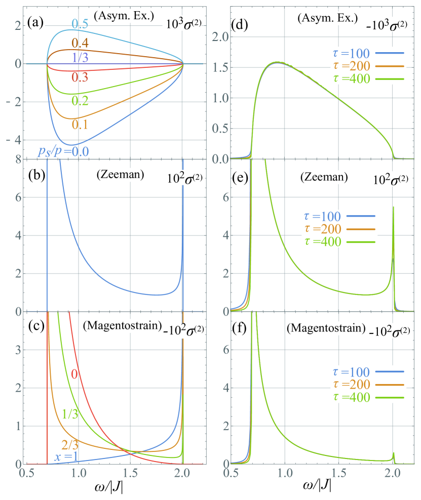
Figure 2: (Color online) Frequency dependence of the nonlinear conductivity $\sigma^{(2)}(\omega)$ for $J=1$, $\delta=1/3$, and $h_{s}=1/10$. Figures (a)-(c) are the results for $\tau\to\infty$ with (a) inverse Dzyaloshinskii-Moriya coupling with $p=1$, (b) Zeeman coupling, and (c) magnetostriction effect with $A=x$ and $A_{s}=1-x$. Different lines in (a) and (c) are the results for different ratio of parameters $p_{s}/p$ and $A/B$, respectively. Figures (d)-(f) shows the $\tau$ dependence of (d) inverse DM coupling with $p=1$ and $p_{s}=0.2$, (e) Zeeman coupling, and (f) magnetostriction effect with $A=1/3$ and $A_{s}=2/3$.

We find that the nonlinear conductance in Eq. (7) shows a characteristic structure when the frequency is close to $\Delta$, i.e., close to the lowest frequency with non-zero $\Re[\sigma^{(2)}(\omega)]$. The asymptotic form of $\Re[\sigma^{(2)}(\omega)]$ reads $\sigma^{(2)}(\omega)\propto\sqrt{\delta\omega}$, where $\delta\omega=\omega-\Delta$ suppl . This frequency dependence is related to the momentum dependence of $g(k)\equiv B_{+-}(k)J_{-+}(k)[B_{--}(k)-B_{++}(k)]$ at the band edge. The real part of $g(k)$ is always zero in our model. Therefore, Eq. (6) becomes

$$\sigma^{(2)}(\omega)= \frac{1}{8}\frac{\Im[g(k_{0}+k_{\omega})]}{\varepsilon_{+}(k_{0}+k_{\omega})}\rho[\varepsilon_{+}(k_{0}+k_{\omega})],$$ (8)

where $\rho(\varepsilon)$ is the density of states (DOS) and $k_{\omega}>0$ is a wavenumber such that $\omega=\varepsilon_{+}(k_{0}+k_{\omega})-\varepsilon_{-}(k_{0}+k_{\omega})$. Here, $k_{0}$ is the location of the band bottom; it is $k_{0}=\pi/2$ ($k_{0}=0$) when $1>\delta^{2}$ ($1<\delta^{2}$). By definition, $\delta\omega=\varepsilon_{+}(k_{0}+k_{\omega})-\varepsilon_{-}(k_{0}+k_{\omega})-\Delta$ and $k_{\omega}\to 0$ when $\delta\omega\to 0$. The asymptotic form $g(k_{0}+k_{\omega})\propto k_{\omega}^{n}$ makes $\sigma^{(2)}(\omega)\propto\delta\omega^{\frac{n-1}{2}}$ through the relations $\delta\omega\propto k_{\omega}^{2}$ and $\rho\propto 1/\sqrt{\delta\omega}$. For the present case, $g(k_{0}+k_{\omega})\propto k_{\omega}^{2}$ leads to $\sigma^{(2)}(\omega)\propto\sqrt{\delta\omega}$. In other words, the asymptotic form of $\sigma^{(2)}(\omega)$ reflects $g(k)$, i.e., $B_{\alpha\beta}(k)$. As shown below, different asymptotic form of $g(k)$ and $\sigma^{(2)}(\omega)$ appears for different kinds of spin-light couplings.

Zeeman coupling — The Zeeman coupling also contributes to the spin current. We here consider an oscillating magnetic field $B(t)=B\cos(\omega t)$ parallel to the magnetic moments. The Hamiltonian reads:

$$H_{\text{Z}}= -B(t)\sum_{i}(\eta-(-1)^{i}\eta_{s})S_{i}^{z}.$$ (9)

This is in contrast to the case of usual spin pumping Kajiwara2010 ; Heinrich2011 ; Ohnuma2014 , in which an oscillating magnetic field perpendicular to the magnetic moment is considered. The spin current is calculated using Eq. (6) by the replacement $B_{\alpha\beta}(k)\to\left<\alpha k\right|H_{\text{Z}}\left|\beta k\right>$. The result reads

$$\sigma^{(2)}(\omega)=\frac{8{\rm sgn}(1-\delta^{2})\delta\,J^{4}h_{s}\eta_{s}^{2}}{\pi\omega^{2}\sqrt{\left(\omega^{2}-\Delta_{\frac{\pi}{2}}^{2}\right)\left(\Delta_{0}^{2}-\omega^{2}\right)}},$$ (10)

at $T=0$ and $\tau\to\infty$. The photocurrent depends on the staggered magnetic field $\eta_{s}$ and not to $\eta$. This follows from the form of the two-band equation in Eq. (6). Naively, three terms appear for $H_{\text{Z}}$, which are proportional to $\eta_{s}^{2}$, $\eta\,\eta_{s}$, and $\eta^{2}$. However, the $\eta\eta_{s}$ term has $B_{\alpha\beta}(k)=\eta\hat{1}_{\alpha\beta}$ for one of the two $B_{\alpha\beta}(k)$’s in Eq. (6) [$B_{+-}(k)$ or $B_{--}(k)-B_{++}(k)$]. As $B_{+-}(k)=B_{--}(k)-B_{++}(k)=0$ for $B_{\alpha\beta}(k)=\eta\hat{1}_{\alpha\beta}$, the $\eta\,\eta_{s}$ term vanishes. Similarly, the $\eta^{2}$ term also vanishes. Hence, only the staggered magnetic field contributes to the spin current.

A notable difference from the inverse DM case appears at the lower edge of the spectrum at $\omega=\Delta$. Figure 2(b) shows the result of $\sigma^{(2)}$ for $\eta_{s}=1$. The conductivity shows a divergence; the asymptotic form is $\sigma^{(2)}(\omega)\propto 1/\sqrt{\delta\omega}$ suppl . The divergence is a consequence of the asymptotic form of $g(k)$, which behaves differently from the asymmetric exchange case; $g(k)$ for the Zeeman coupling become a constant when $\omega\searrow\Delta$. The substitution of $g(k)$ into Eq. (8) gives the asymptotic form $\sigma^{(2)}\propto\rho(k_{\omega})\propto\delta\omega^{-1/2}$. Hence, the divergence reflects the structure of the DOS.

Magnetostriction effect — Magnetostriction effect also leads to a coupling between local exchange interaction and an external electromagnetic field Tokura2014 ; Pimenov2006 ; Miyahara2008 ; Mochizuki2010-2 ; Katsura2009 ; Furukawa2010 ; the Hamiltonian reads

$$H_{\text{ms}}=E_{x}(t)\sum_{i}\{A+(-1)^{i}A_{s}\}(S_{i}^{x}S_{i+1}^{x}+S_{i}^{y}S_{i+1}^{y}).$$ (11)

Here, $A$ and $A_{s}$ are the uniform and staggered magnetostriction terms, respectively, and $E_{x}(t)=E_{x}\cos(\omega t)$ is the oscillating electric field along the $x$ axis. $A$ ($A_{s}$) is the magnetostriction effect for $J$ ($J\delta$).

The solution for $H_{\text{ms}}$ at $T=0$ and $\tau\to\infty$ reads

$$\sigma^{(2)}(\omega)= -\frac{{\rm sgn}(1-\delta^{2})h_{s}}{4\pi\omega^{2}J^{2}(1-\delta^{2})^{2}\sqrt{(\omega^{2}-\Delta_{\frac{\pi}{2}}^{2})(\Delta_{0}^{2}-\omega^{2})}}$$

$$\times\left\{A(\Delta_{\frac{\pi}{2}}^{2}-\omega^{2})+A_{s}\delta(\omega^{2}-\Delta_{0}^{2})\right\}$$

$$\times\left\{A_{s}(\Delta_{0}^{2}-\omega^{2})+A\delta(\omega^{2}-\Delta_{\frac{\pi}{2}}^{2})\right\}.$$ (12)

Figure 2(c) shows the $\omega$ dependence of $\sigma^{(2)}(\omega)$ for $J=1$, $\delta=1/3$, and $h_{s}=1/10$. Unlike the other two cases, the asymptotic structure at $\omega\sim\Delta$ changes depending on $A$ and $A_{s}$. When $\delta^{2}<1$, a divergent structure similar to the Zeeman coupling, $\sigma^{(2)}(\omega)\approx\frac{1}{\sqrt{\delta\omega}}$, appears for $A_{s}\neq 0$. On the other hand, the conductivity smoothly goes to zero at $\omega=\Delta$ for $A_{s}=0$; in this case, $\sigma^{(2)}(\omega)\approx\delta\omega^{\frac{3}{2}}$ at the lower edge. Therefore, the magnetostriction effect also contributes to the spin current with a characteristic behavior at the lower edge $\omega\sim\Delta$. Further details are presented in the supplementary information suppl .

Relaxation time dependence — The $\tau$ dependence of a light-induced current often reflects its microscopic mechanism. For instance, in the study of photovoltaic effect, shift current does not depend on $\tau$ while the injection current is linearly proportional to $\tau$ Sturman1992 ; Sipe2000 . The numerical results of $\sigma^{\text{(2)}}(\omega)$ for different $\tau$ are shown in Figs. 2(d)-(f); each figure shows the results for (d) asymmetric exchange, (e) Zeeman, and (f) magnetostriction couplings. All results are calculated using $L=2^{14}$ site chains with periodic boundary condition. The result shows that the photo spin current is insensitive against the value of $\tau$. Therefore, the spin current is robust against the suppression of the relaxation time. This behavior is similar to the shift current in electronic photogalvanic effects.

Discussion — In this work, we explored the generation of spin current using nonlinear response. To this end, we considered simple but realistic quantum spin chains with three different types of couplings between spins and electromagnetic field: Inverse DM, Zeeman, and magnetostriction couplings. The spin current generated by all three mechanisms is independent of relaxation time of the magnetic excitation. However, our simple model shows the spin current appears from different microscopic processes compared with the relaxation-time-independent electronic photocurrent (shift current) Kraut1979 ; Belinicher1982 ; Sipe2000 . This feature is crucial for magnets as the total number of the bands are much less than the electronic bands. Therefore, our proposal for the spin current is generally expected in simple magnetic structures.

Another interesting feature is the anisotropy of the spin current. In our model, the spin current by inverse DM and magnetostriction couplings can be switched by rotating the electric field; the field along $y$ axis gives inverse DM component while $x$ gives the magnetostriction. Similarly, Zeeman coupling contributes when the magnetic field along $z$ axis. This anisotropy in the microscopic mechanism is reflected in the frequency dependence. Experimentally, the obseravtion of the anisotropy distinguishes the microscopic mechanism of the spin current.

We also stress that the mechanism of generating spin current differs from spin pumping Kajiwara2010 ; Heinrich2011 ; Ohnuma2014 . Unlike the spin pumping, all three mechanisms we considered preserves the spin angular momentum along $z$ axis. Therefore, in contrast to the spin pumping, no angular momentum is supplied from the electromagnetic waves. The conservation decidedly shows that the spin current studied here is by the nontrivial motion of magnetic excitations.

In the last, we estimate the order of the spin current for each of the contributions. A typical value of exchange interactions are used for the estimate: $J\sim 10^{2}k_{B}$ J, $\delta\sim 0.1$, and $h_{s}\sim\mu_{B}$ J. The relative permittivity $\epsilon_{r}=10$ is assumed. The excitation gap for these values reads $\Delta_{g}=\Delta_{\frac{\pi}{2}}\sim 1$meV. Therefore, the frequency of the light is assumed to be $\omega\sim\Delta_{\frac{\pi}{2}}/\hbar\sim 1$ terahertz. Using these values, we compute the strength of the oscillating electric field required for the spin current density $J^{(0)}_{sc}=10^{-16}$ J/cm². Here $J_{sc}^{(0)}$ is an expected, typical value of the spin current observed in a recent experiment of the spin Seebeck effect for a quasi-1D magnet $\rm Sr_{2}CuO_{3}$ suppl ; Hirobe2017 . For the inverse DM coupling, the magnitude of the electric polarization $p\sim 10^{-31}$ Cm and $p_{s}\sim 10^{-32}$ Cm are used Jia2006 ; Ishizuka2018 . A bulk solid of the spin chains aligned with $\sim a_{0}=4$Å  distance gives the nonlinear conductivity $\sigma_{3D}^{(2)}\equiv\sigma^{(2)}/a_{0}^{2}\sim 10^{-25}$ A²s⁴/m²kg. Therefore, $E_{y}=\epsilon_{r}(J_{sc}^{(0)}/\sigma_{3D}^{(2)})^{1/2}\sim 10^{5}$ V/cm is required so that the spin current approaches the value of $J_{sc}^{(0)}$. Similarly, in the case of Zeeman coupling, the staggered moment $\eta_{s}\sim 0.1\mu_{B}$ J/T gives $\sigma_{3D}^{(2)}\sim 10^{-9}$ J/T²m². This requires $B\sim 10^{-2}$ T (or $E\sim 10^{4}$ V/cm) to induce $J_{sc}^{(0)}$. In the last, the magnetostriction coupling with $A\sim A_{s}\sim 10^{-28}$ Jm/V suppl gives $\sigma_{3D}^{(2)}\sim 10^{-19}$ A²s⁴/m²kg and $E\sim 10^{2}$ V/cm. Therefore, the spin current generated by all three mechanisms should be observable in experiments.

This work was supported by JSPS KAKENHI (Grant Numbers JP16H06717, JP18H03676, JP18H04222, JP26103006, JP17K05513 and No. JP15H02117), ImPACT Program of Council for Science, Technology and Innovation (Cabinet office, Government of Japan), CREST JST (Grant No. JPMJCR16F1), and Grant-in-Aid for Scientific Research on Innovative Area “Nano Spin Conversion Science”(Grant No.17H05174).

References

- (1) Spin Current, edited by S. Maekawa, S. O. Valenzuela, E. Saitoh, and T. Kimura (Oxford University Press, Oxford, England, 2012).
- (2) L. Berger, J. Appl. Phys. 55, 1954 (1984).
- (3) M. I. Dyakonov and V. I. Perel, JETP Lett. 13, 467 (1971).
- (4) J. E. Hirsch, Phys. Rev. Lett. 83, 1834 (1999).
- (5) S. Murakami, N. Nagaosa, and S.-C. Zhang, Science 301, 1348 (2003).
- (6) J. Sinova, D. Culser, Q. Niu, N. A. Sinitsyn, T. Jungwirth, and A. H. MacDonald, Phys. Rev. Lett. 92, 16603 (2004).
- (7) A. V. Kimel, A. Kirilyuk, P. A. Usachev, R. V. Pisarev, A. M. Balbashov, and T. Rasing, Nature 435, 655 (2005).
- (8) C. D. Stanciu, F. Hansteen, A. V. Kimel, A. Kirilyuk, A. Tsukamoto, A. Itoh, T. Rasing, Phys. Rev. Lett. 99, 047601 (2007).
- (9) A. Kirilyuk, A. V. Kimel, and T. Rasing, Rev. Mod. Phys. 82, 2731 (2010).
- (10) Y. Mukai, H. Hirori, T. Yamamoto, H. Kageyama, and K. Tanaka, New J. Phys. 18, 013045 (2016).
- (11) S. Takayoshi, H. Aoki, and T. Oka, Phys. Rev. B 90, 085150 (2014).
- (12) S. Takayoshi, M. Sato, and T. Oka, Phys. Rev. B 90, 214413 (2014).
- (13) J. H. Mentink, K. Balzer, and M. Eckstein, Nature Commun. 6, 6708 (2015).
- (14) M. Mochizuki and N. Nagaosa, Phys. Rev. Lett. 105, 147202 (2010).
- (15) W. Koshibae and N. Nagaosa, Nature Commun. 5, 5148 (2014).
- (16) M. Sato, S. Takayoshi, and T. Oka, Phys. Rev. Lett. 117, 147202 (2016).
- (17) H. Fujita and M. Sato, Phys. Rev. B 95, 054421 (2017).
- (18) H. Fujita and M. Sato, Phys. Rev. B 96, 060407(R) (2017).
- (19) A. Ono and S. Ishihara, Phys. Rev. Lett. 119, 207202 (2017).
- (20) T. Satoh, Y. Terui, R. Moriya, B. A. Ivanov, K. Ando, E. Saitoh, T. Shimura, and K. Kuroda, Nature Photon. 6, 662 (2012).
- (21) Y. Hashimoto, S. Daimon, R. Iguchi, Y. Oikawa, K. Shen, K. Sato, D. Bossini, Y. Tabuchi, T. Satoh, B. Hillebrands, G. E. W. Bauer, T. H. Jo-hansen, A. Kirilyuk, T. Rasing, and E. Saitoh, Nature Commun. 8, 15859 (2017).
- (22) P. Ňemec, M. Fiebig, T. Kampfrath, and A. V. Kimel, Nature Phys. 14, 229 (2018).
- (23) Y. Kajiwara, K. Harii, S. Takahashi, J. Ohe, K. Uchida, M. Mizuguchi, H. Umezawa, H. Kawai, K. Ando, K. Takanashi, S. Maekawa and E. Saitoh, Nature 464, 262 (2010).
- (24) B. Heinrich, C. Burrowes, E. Montoya, B. Kardasz, E. Girt, Young-Yeal Song, Yiyan Sun, and M. Wu, Phys. Rev. Lett. 107, 066604 (2011).
- (25) Y. Ohnuma, H. Adachi, E. Saitoh, and S. Maekawa, Phys. Rev. B 89, 174417 (2014).
- (26) B. I. Sturman and V. M. Fridkin, “The photovoltaic and photorefractive effects in noncentrosymmetric materials”, (Gordon and Breach Science Publishers, 1992).
- (27) L. Z. Tan, F. Zheng, S. M. Young, F. Wang, S. Liu, and A. M. Rappe, NPJ Comput. Mater. 2, 16026 (2016).
- (28) Y. Tokura and N. Nagaosa, Nature Commun. 9, 3740 (2018).
- (29) V. Belinicher, E. L. Ivcheriko, and B. Sturman, Zh. Eksp. Teor. Fiz. 83, 649 (1982).
- (30) J. E. Sipe and A. I. Shkrebtii, Phys. Rev. B 61, 5337 (2000)
- (31) T. Morimoto and N. Nagaosa, Sci. Adv. 2, e1501524 (2016).
- (32) H. Ishizuka and N. Nagaosa, New J. Phys. 19, 033015 (2017).
- (33) M. Nakamura, S. Horiuchi, F. Kagawa, N. Ogawa, T. Kurumaji, Y. Tokura, and M. Kawasaki, Nature Commun. 8, 281 (2017).
- (34) N. Ogawa, M. Sotome, Y. Kaneko, M. Ogino, and Y. Tokura, Phys. Rev. B 96, 241203 (2017).
- (35) D. C. Dender, P. R. Hammar, D. H. Reich, C. Broholm, and G. Aeppli, Phys. Rev. Lett. 79, 1750 (1997).
- (36) M. Oshikawa, K. Ueda, H. Aoki, A. Ochiai, and M. Kohgi, J. Phys. Soc. Jpn. 68, 3181 (1999).
- (37) R. Feyerherm, S. Abens, D. Günther, T. Ishida, M. Meisner, M. Meschke, T. Nogami, and M. Steiner, J. Phys.: Condens. Matter 12, 8495 (2000).
- (38) R. Morisaki, T. Ono, H. Tanaka, and H. Nojiri, J. Phys. Soc. Jpn. 76, 063706 (2007).
- (39) I. Umegaki, H. Tanaka, T. Ono, H. Uekusa, and H. Nojiri, Phys. Rev. B 79, 184401 (2009).
- (40) I. Affleck and M. Oshikawa, Phys. Rev. B 60, 1038 (1999); 62, 9200 (2000).
- (41) N. Ishimura, and H. Shiba, Prog. Theor. Phys. 63, 743 (1980).
- (42) R. Coldea, D. A. Tennant, E. M. Wheeler, E. Wawrzynska, D. Prabhakaran, M. Telling, K. Habicht, P. Smeibidl, K. Kiefer, Science 327 177 (2010).
- (43) Q. Faure, S. Takayoshi, S. Petit, V. Simonet, S. Raymond, L-P. Regnault, M. Boehm, J. S. White, M. Mânsson, C. R’́uegg, P. Lejay, B. Canals, T. Lorenz, S. C. Furuya, T. Giamarchi and B. Grenier, Nature Phys. 14, 716 (2018).
- (44) D. J. Scalapino, Y. Imry, and P. Pincus, Phys. Rev. B 11, 2042 (1975).
- (45) H. J. Schulz, Phys. Rev. Lett. 77, 2790 (1996).
- (46) M. Sato and M. Oshikawa, Phys. Rev. B 69, 054406 (2004).
- (47) K. Okunishi and T. Suzuki, Phys. Rev. B 76, 224411 (2007).
- (48) T. Giamarchi, Quantum Physics in One Dimension, (Oxford University Press, New York, 2003).
- (49) A. O. Gogolin, A. A. Nersesian, and A. M.Tsvelik, Bosonization and strongly correlated systems, (Cambridge University Press, UK, 2004).
- (50) A. M. Tsvelik, Quantum Field Theory in Condensed Matter Physics, (Cambridge University Press, UK, 2007).
- (51) H. Katsura, N. Nagaosa, and A. V. Balatsky, Phys. Rev. Lett. 95, 057205 (2005).
- (52) Y. Takahashi, R. Shimano, Y. Kaneko, H. Murakawa, and Y. Tokura, Nature Phys. 8, 121 (2012).
- (53) D. H’́uvonen, U. Nagel, T. Rõõm, Y. J. Choi, C. L. Zhang, S. Park, and S.-W. Cheong, Phys. Rev. B 80, 100402(R) (2009).
- (54) S. Furukawa, M. Sato, and S. Onoda, Phys. Rev. Lett. 105, 257205 (2010).
- (55) Y. Tokura, S. Seki, and N. Nagaosa, Rep. Prog. Phys. 77, 076501 (2014).
- (56) W. Kraut and R. von Baltz, Phys. Rev. B 19, 1548 (1979).
- (57) Supplemental information.
- (58) A. Pimenov, A. A. Mukhin, V. Yu. Ivanov, V. D. Travkin, A. M. Balbashov and A. Loidl, Nature Phys. 2, 97 (2006).
- (59) S. Miyahara and N. Furukawa, arXiv:0811.4082.
- (60) M. Mochizuki, N. Furukawa, and N. Nagaosa, Phys. Rev. Lett. 104, 177206 (2010).
- (61) H. Katsura, M. Sato, T. Furuta, and N. Nagaosa, Phys. Rev. Lett. 103, 177402 (2009).
- (62) D. Hirobe, M. Sato, T. Kawamata, Y. Shiomi, K. Uchida, R. Iguchi, Y. Koike, S. Maekawa, and E. Saitoh, Nature Phys. 13, 30 (2017).
- (63) C. Jia, S. Onoda, N. Nagaosa, and J. H. Han, Phys. Rev. B 74, 224444 (2006).
- (64) H. Ishizuka and N. Nagaosa, preprint (arXiv:1806.06833) (2018).