The COMPASS force field: validation for carbon nanoribbons.

Abstract

The COMPASS force field has been successfully applied in a large number of materials simulations, including the analysis of structural, electrical, thermal, and mechanical properties of carbon nanoparticles. This force field has been parameterized using quantum mechanical data and is based on hundreds of molecules as a training set, but such analysis for graphene sheets was not carried out. The objective of the present study is the verification of how good the COMPASS force field parameters can accurately describe the frequency spectrum of atomic vibrations of graphene, graphane and fluorographene sheets. We showed that the COMPASS force field allows to describe with good accuracy the frequency spectrum of atomic vibrations of graphane and fluorographene sheets, whose honeycomb hexagonal lattice is formed by sp³ hybridization. On the other hand, the force field doesn’t describe very well the frequency spectrum of graphene sheet, whose planar hexagonal lattice is formed by sp² banding. In that case the frequency spectrum of out-of-plane vibrations differs greatly from the experimental data – bending stiffness of a graphene sheet is strongly over estimated. We present the correction of parameters of out-of-plane and torsional potentials of the force field, that allows to achieve the coincidence of vibration frequency with experimental data. After such corrections the COMPASS force field can be used to describe the dynamics of flat graphene sheets and carbon nanotubes.

I Introduction

The obtaining of the monolayer graphene membrane with the unique physical properties pm1 caused the unprecedented rise in research of single and multilayer graphene sheets, graphene nanoribbons and nanoscrolls, other graphene-based and functional graphene nanostructures pm2 ; pm3 ; pm4 ; pm5 ; pm6 ; pm7 ; pm8 . The possibility of using such structures in electronics pm9 ; pm10 , optics pm11 , and in many other industries has been much discussed recently pm5 ; pm7 ; pm12 ; pm13 ; pm14 ; pm15 ; pm16 . The remarkable properties of graphene make it one of the key components in creating nanomaterials for energy storage pm17 ; pm18 ; pm10 ; pm20 , polymer nanocomposites pm2 ; pm21 and for medicine pm22 ; pm23 .

Experimental studies of these nanostructures are difficult because of their small size. So particular attention is paid to their computer simulation, where quantum mechanics (QM) equations, molecular dynamics (MD) or molecular mechanics (MM) equations are used. QM simulation allows to consider only small-sized molecular structures, but enables to justify empirical interatomic potentials in MM/MD modelling. However, the accuracy of MD simulations depends on parametrization of the empirical potentials that describe the atomic interactions. Both experimental data and results of QM calculation used for determination of these parameters. For MM/MD modelling carbon nanoforms a variety of carbon interatomic potentials have been used. Examples of the carbon potentials are reactive empirical bond-order potential REBO/AIREBO pm24 ; pm25 ; pm26 ; pm27 , reactive force field ReaxFF pm28 , long-range carbon bond order potential LCBOP pm29 , an analytical bond order potential (BOP) pm30 , environment dependent interatomic potential (EDIP) pm31 , the modified embedded atom method (MEAM) potential pm32 , the DREIDING force field pm33 , Morse force field pm34 ; pm35 .

It is assumed that the force field parameters should reproduce the value of mechanical moduli and vibration spectrum of nanoparticles, but the standard parameter sets of the above-mentioned force fields have been received taking into account only in-plane frequency spectrum or/and in-plane molecular mechanics. Taking into account out-of-plane vibrations made it possible to significantly improve the matching of the bending rigidity modulus and dispersion curves calculated in MD with the available experimental data and QM simulation for force fields Morse pm36 ; pm37 , MEAM pm38 and DREIDING pm39 .

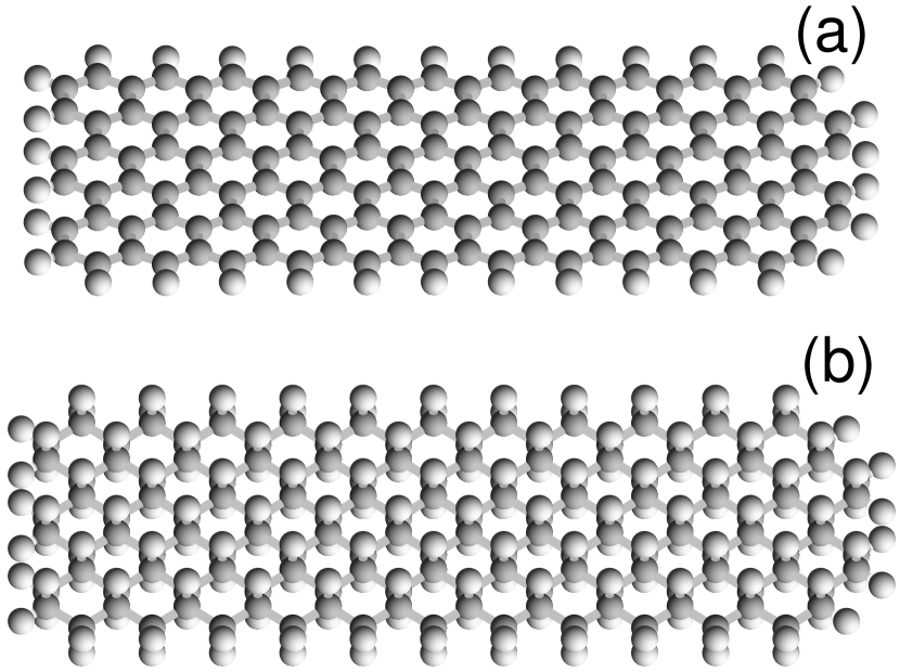
Figure 1: Structures of nanoribbons (a) graphene (C₁₂H₂)₁₁C₁₀H₁₂ (of size $29.9\times 13.4$Ų) and (b) graphane (C₁₂H₁₄)₁₁C₁₀H₂₂ (of size $29.1\times 11.7$Ų).

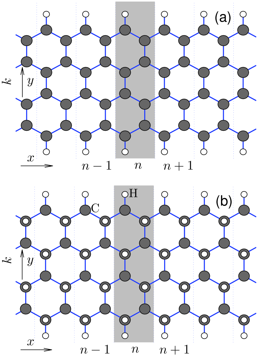
Figure 2: Schematic view of the structures of zigzag (a) graphene (C₈H₂)_∞ and (b) graphane (C₈H₁₀)_∞ nanoribbons. The indices $n$ and $k$ enumerate the unit cells in the nanoribbon and the atoms in the cell. Dotted lines indicate the cell borders. Gray color region is the elementary cell of the nanoribbon. Nanoribbons lie on the $xy$-plane.

A condensed-phase optimised ab-initio COMPASS force field has been developed recently pm40 ; pm41 and has been successfully applied in a large number of soft materials simulations with carbon nanostructures (see pm42 ; pm43 ; pm44 ; pm45 ; pm46 ; pm47 ; pm48 ; pm49 and references in them). The force field has been parameterized using hundreds of molecules as a training set including molecules with sp³- and sp²-hybridized carbon atoms, but the parameterization and validation using planner monomolecular lattice structures as graphene sheets and its modifications have not been yet performed.

The purpose of article is to checking how well force field of the COMPASS reproduces a vibration range of three nanoribbons: graphene, graphane and fluorographene. For this we calculated the frequency spectrum and dispersion curves of these nanoribbons using the COMPASS force field, and compared them with results of ab-initio data. It was found that the force field could give an accurate reproduction of experimental spectrum lattice of sp³ hybridization, such as graphene or fluorographene. However, the obtained frequency spectrum of graphene turned out to be noticeably shifted to the high-frequency region with respect to the known theoretical and experimental data for out-of-plane vibrations of carbon. We made a correction of parameters of torsional potentials, what allowed to rectify that deficiency of the COMPASS force field.

Table 1: Values of the parameters for valence bond potential $V_{1}(b)=k_{b,2}(b-b_{0})^{2}+k_{b,3}(b-b_{0})^{3}+k_{b,4}(b-b_{0})^{4}$, angle potential $V_{2}(\theta)=k_{\theta,2}(\theta-\theta_{0})^{2}+k_{\theta,3}(\theta-\theta_{0})^{3}+k_{\theta,4}(\theta-\theta_{0})^{4}$ and torsional potential $V_{t}(\phi)=k_{\phi,1}(1-\cos\phi)+k_{\phi,2}(1-\cos 2\phi)+k_{\phi,3}(1-\cos 3\phi)$.

Bond	$b_{0}$ (Å)	$k_{b,2}$ (kcal/mol$\cdot$Å2)	$k_{b,3}$ (kcal/mol$\cdot$Å3)	$k_{b,4}$ (kcal/mol$\cdot$Å4)
CC (sp2 atoms)	1.4170	470.8361	-627.6179	1327.6345
CH (sp2 atoms)	1.0982	372.8251	-803.4526	894.3173
CC (sp3 atoms)	1.530	299.670	-501.77	679.81
CH (sp3 atoms)	1.101	345.000	-691.89	844.60
CF (sp3 atoms)	1.390	403.032	0	0
Angle	$\theta_{0}$ (deg)	$k_{\theta,2}$ (kcal/mol$\cdot$rad2)	$k_{\theta,3}$ (kcal/mol$\cdot$rad3)	$k_{\theta,4}$ (kcal/mol$\cdot$rad4)
CCC (sp2 atoms)	118.90	61.0226	-34.9931	0
CCH (sp2 atoms)	117.94	35.1558	-12.4682	0
CCC (sp3 atoms)	112.67	39.5160	-7.4430	-9.5583
CCH (sp3 atoms)	110.77	41.4530	-10.6040	5.1290
HCH (sp3 atoms)	107.66	39.6410	-12.9210	-2.4318
CCF (sp3 atoms)	109.20	68.3715	0	0
FCF (sp3 atoms)	109.10	71.9700	0	0
Torsion	$k_{\phi,1}$ (kcal/mol)	$k_{\phi,2}$ (kcal/mol)	$k_{\phi,3}$ (kcal/mol)
CCCC (sp2 atoms)	8.3667	1.2000	0
CCCH (sp2 atoms)	0	3.9661	0
HCCH (sp2 atoms)	0	2.3500	0
CCCC (sp3 atoms)	0	0.0514	-0.1430
CCCH (sp3 atoms)	0	0.0316	-0.1681
CCCF (sp3 atoms)	0	0	0.1500
HCCH (sp3 atoms)	-0.1432	0.0617	-0.1530
FCCF (sp3 atoms)	0	0	-0.1

II A model of a graphene and graphane nanoribbons

Molecular nanoribbon is a narrow, straight-edged strip, cut from a single-layered molecular plane. The simplest example of such molecular plane is a graphene sheet (isolated monolayer of carbon atoms of crystalline graphite) and its various chemical modifications: graphane (fully hydrogenated on both sides graphene sheet) and fluorographene (fluorinated graphene). As is known, graphene and its modifications are elastically isotropic materials, the longitudinal and flexural rigidity of which is weakly dependent on chirality of the structure. Therefore, for definiteness, we will consider nanoribbons with the zigzag structure shown in Fig. 1 and 2.

Let us consider a rectangular ribbon cut from a flat sheet of graphene [Fig. 1 (a)] and graphane [Fig. 1 (b)] in the zigzag directions. The nanoribbons structure can be obtained by longitudinal translation of a transverse unit cell consisting of $N_{e}=N_{\rm C}+N_{\rm H}$ atoms (see Fig. 2). Number of the carbon atoms in the unit cell is always multiple of two, and number of hydrogen atoms $N_{\rm H}=2$ for graphene nanoribbon and $N_{\rm H}=N_{\rm C}+2$ for graphane. Further we use the following notation (see Fig. 2): each atom is numbered with at two-component index $\alpha=(n,k)$, where $n=0,\pm 1,\pm 2,...$ defines the unit cell number and $k=1,...,N_{e}$ numbers atoms in the unit cell.

For numerical simulation we will use COMPASS force-field functional form pm40 :

$$E_{total}=\sum_{b}[k_{b,2}(b-b_{0})^{2}+k_{b,3}(b-b_{0})^{3}+k_{b,4}(b-b_{0})^{4}]$$

$$+\sum_{\theta}[k_{\theta,2}(\theta-\theta_{0})^{2}+k_{\theta,3}(\theta-\theta_{0})^{3}+k_{\theta,4}(\theta-\theta_{0})^{4}]$$

$$+\sum_{\phi}[k_{\phi,1}(1-\cos\phi)+k_{\phi,2}(1-\cos 2\phi)$$

$$+k_{\phi,3}(1-\cos 3\phi)]$$

$$+\sum_{\chi}k_{\chi}\chi^{2}+\sum_{bb^{\prime}}k_{bb^{\prime}}(b-b_{0})(b^{\prime}-b_{0}^{\prime})$$

$$+\sum_{b,\theta}k_{b\theta}(b-b_{0})(\theta-\theta_{0})+\sum_{\theta,\theta^{\prime}}k_{\theta\theta^{\prime}}(\theta-\theta_{0})(\theta^{\prime}-\theta_{0}^{\prime})$$

$$+\sum_{b,\phi}(b-b_{0})[k_{b\phi,1}\cos\phi+k_{b\phi,2}\cos 2\phi+k_{b\phi,3}\cos 3\phi]$$

$$+\sum_{\theta,\phi}(\theta-\theta_{0})[k_{\theta\phi,1}\cos\phi+k_{\theta\phi,2}\cos 2\phi+k_{\theta\phi,3}\cos 3\phi]$$

$$+\sum_{\theta,\theta^{\prime},\phi}k_{\theta\theta^{\prime}\phi}(\theta-\theta_{0})(\theta^{\prime}-\theta_{0}^{\prime})\cos\phi$$

$$+\sum_{i,j}q_{i}q_{j}/r_{ij}+\sum_{i,j}\epsilon_{ij}[2(r_{ij}^{0}/r_{ij})^{9}-3(r_{ij}^{0}/r_{ij})^{6}].~{}~{}~{}~{}~{}~{}$$ (1)

The functions could be divided into two categories: (1) valence terms including diagonal and off-diagonal cross-coupling terms and (2) nonbonded interactions terms. The valence terms represent internal coordinates of bond $b$, angle $\theta$, torsion angle $\phi$, and out-of-plane angle $\chi$, and the cross-coupling terms include combinations of two or three internal coordinates. The nonbond interactions include a LJ-9-6 potentials for the van der Waals (vdW) term and a Coulombic potential for an electrostatic interaction.

Graphene has a flat form due to the sp² hybridization of all valence bonds [Fig. 1 (a)]. Graphane (fully hydrogenated graphene) as a two-dimensional crystal was predicted in theoretical works pm50 ; pm51 and was confirmed by experimental data in pm52 . Graphane is an analogue of graphene with the unique properties pm53 ; pm54 ; pm55 ; pm56 . Graphane nanoribbon is a strip with a constant width cut from a two-sized hydrogenated graphene sheet [see Fig. 1 (b), 2 (b)]. Several conformations of the graphane sheet are existed, and we consider the most energy-efficient configuration armchair, where hydrogen atoms are connected from different sides to all adjacent carbon atoms. Substitution of hydrogen atoms for fluorine atoms leads to formation of the fluorographene sheet structure (fully fluorinated graphene). In comparison with graphene, graphane and fluorographene are not two-dimensional crystal structures, but corrugated sheets with sp³ hybridized carbon atoms and with atoms of hydrogen or fluorine connected to the different sides of the sheet.

For graphene nanoribbon simulation the potentials (1) with the parameters of atom with sp² hybridization should be used, and for graphane and fluorographene nanoribbon simulation – potentials with the parameters of atom with sp³ hybridization. There quired parameters for interatomic interaction potentials are shown in Tabl. 1. Out-of-plane angle potential $V_{3}(\chi)=k_{\chi}\chi^{2}$ appears in the Hamiltonian only for graphene nanoribbons with planar sp² valence bands: for C–C–C–C atom group $\kappa_{\chi}=7.1794$ kcal/mol, for C–C–C–H atoms $\kappa_{\chi}=4.8912$ kcal/mol. Parameters for cross-coupling interactions potentials are shown in Tables 2 and 3. Parameters for nonvalence interactions can be found in Table 4. Parameters values for C and H atoms are taken from pm40 , for fluorine atom the parameters values – from force field CFF91.

Table 2: Values of parameters for cross-coupling bond/bond potential $V(b,b^{\prime})=k_{bb^{\prime}}(b-b_{0})(b^{\prime}-b_{0}^{\prime})$, bond/angle potential $V(b,\theta)=k_{b\theta}(b-b_{0})(\theta-\theta_{0})$ angle/angle potential, $V(\theta,\theta^{\prime})=k_{\theta\theta^{\prime}}(\theta-\theta_{0})(\theta^{\prime}-\theta_{0}^{\prime})$ and angle/angle/torsion potential $V(\theta,\theta^{\prime},\phi)=k_{\theta\theta^{\prime}\phi}(\theta-\theta_{0})(\theta^{\prime}-\theta_{0}^{\prime})\cos\phi$

bond/bond	$k_{bb^{\prime}}$ (kcal/mol$\cdot$Å2)
CC/CC (first neighboring, sp2)	68.2856
CC/CH (first neighboring, sp2)	1.0795
CC/CC (second neighboring, sp2)	53.0
CC/CH (second neighboring, sp2)	-6.2741
CH/CH (second neighboring, sp2)	-1.7077
CC/CH (first neighboring, sp3)	3.3872
CH/CH (first neighboring, sp3)	5.3316
CC/CC (first neighboring, sp3)	0
bond/angle	$k_{b\theta}$ (kcal/mol$\cdot$Å$\cdot$rad)
C–C/C–C–C (sp2 atoms)	28.8708
C–C/C–C–H (sp2 atoms)	20.0033
C–H/C–C–H (sp2 atoms)	24.2183
C–C/C–C–C (sp3 atoms)	8.016
C–C/C–C–H (sp3 atoms)	20.754
C–H/C–C–H (sp3 atoms)	11.421
C–H/H–C–H (sp3 atoms)	18.103
angle/angle	$k_{\theta\theta^{\prime}}$ (kcal/mol$\cdot$rad2)
C–C–C/C–C–C (sp2 atoms)	0
C–C–C/C–C–H (sp2 atoms)	0
H–C–C/C–C–H (sp2 atoms)	0
C–C–C/C–C–C (sp3 atoms)	-0.1729
C–C–C/C–C–H (sp3 atoms)	-1.3199
H–C–C/C–C–H (sp3 atoms)	-0.4825
angle/angle/torsional	$k_{\theta\theta^{\prime}\phi}$ (kcal/mol$\cdot$rad2)
C–C–C/C–C–C/C–C–C–C (sp2)	0
C–C–C/C–C–H/C–C–C–H (sp2)	-4.8141
H–C–C/C–C–H/H–C–C–H (sp2)	0.3598
C–C–C/C–C–C/C–C–C–C (sp3)	-22.045
C–C–C/C–C–H/C–C–C–H (sp3)	-16.164
H–C–C/C–C–H/H–C–C–H (sp3)	-12.564

Table 3: Values of parameters for cross-coupling bond/torsion potential $V(b,\phi)=(b-b_{0})[k_{b\phi,1}\cos\phi+k_{b\phi,2}\cos 2\phi+k_{b\phi,3}\cos 3\phi]$. and cross-coupling angle/torsion potential $V(\theta,\phi)=(\theta-\theta_{0})[k_{\theta\phi,1}\cos\phi+k_{\theta\phi,2}\cos 2\phi+k_{\theta\phi,3}\cos 3\phi]$.

Bond/torsion	$k_{b\phi,1}$ (kcal/mol$\cdot$Å)	$k_{b\phi,2}$ (kcal/mol$\cdot$Å)	$k_{b\phi,3}$ (kcal/mol$\cdot$Å)
C–C/C–C–C–C (sp2 atoms, central bond)	27.5989	-2.3120	0
C–C/C–C–C–H (sp2 atoms, central bond)	0	-1.1521	0
C–H/H–C–C–H (sp2 atoms, central bond)	0	4.8228	0
C–C/C–C–C–C (sp2 atoms, terminal bond)	-0.1185	6.3204	0
C–C/C–C–C–H (sp2 atoms, terminal bond)	0	-6.8958	0
C–H/C–C–C–H (sp2 atoms, terminal bond)	0	-0.4669	0
C–H/H–C–C–H (sp2 atoms, terminal bond)	0	-0.6890	0
C–C/C–C–C–C (sp3 atoms, central bond)	-17.787	-7.1877	0
C–C/C–C–C–H (sp3 atoms, central bond)	-14.879	-3.6581	-0.3138
C–C/H–C–C–H (sp3 atoms, central bond)	-14.261	-0.5322	-0.4864
C–C/C–C–C–C (sp3 atoms, terminal bond)	-0.0732	0	0
C–C/C–C–C–H (sp3 atoms, terminal bond)	0.2486	0.2422	-0.0925
C–H/C–C–C–H (sp3 atoms, terminal bond)	0.0814	0.0591	0.2219
C–H/H–C–C–H (sp3 atoms, terminal bond)	0.2130	0.3120	0.0777
angle/torsion	$k_{\theta\phi,1}$ (kcal/mol$\cdot$rad)	$k_{\theta\phi,2}$ (kcal/mol$\cdot$rad)	$k_{\theta\phi,3}$ (kcal/mol$\cdot$rad)
C–C–C/C–C–C–C (sp2 atoms)	1.9767	1.0239	0
C–C–C/C–C–C–H (sp2 atoms)	0	2.5014	0
C–C–H/C–C–C–H (sp2 atoms)	0	2.7147	0
H–C–C/H–C–C–H (sp2 atoms)	0	2.4501	0
C–C–C/C–C–C–C (sp3 atoms)	0.3886	-0.3139	0.1389
C–C–C/C–C–C–H (sp3 atoms)	-0.2454	0	-0.1136
C–C–H/C–C–C–H (sp3 atoms)	0.3113	0.4516	-0.1988
H–C–C/H–C–C–H (sp3 atoms)	-0.8085	0.5569	-0.2466

Table 4: Values of parameters for LJ-9-6 potential $V(r)=\epsilon[2(r_{0}/r)^{9}-3(r_{0}/r)^{6}]$ and charge valence bond increments $q_{1}$, $q_{2}$

atom atom	$\epsilon$ (kcal/mol)	$r_{0}$ (Å)
C C (sp2 atoms)	0.0680	3.9150
C H (sp2 atoms)	0.0271	3.5741
H H (sp2 atoms)	0.0230	2.878
C C (sp3 atoms)	0.0400	3.854
H H (sp3 atoms)	0.0230	2.878
F F (sp3 atoms)	0.0598	3.200
C H (sp3 atoms)	0.0215	3.526
C F (sp3 atoms)	0.0422	3.600
atom atom	$q_{1}$ (e)	$q_{2}$ (e)
C C (sp2 atoms)	0	0
C H (sp2 atoms)	-0.1268	+0.1268
C C (sp3 atoms)	0	0
C H (sp3 atoms)	-0.053	+0.053
C F (sp3 atoms)	+0.25	-0.25

Taking into consideration the noncovalent interactions of atoms only from neighboring unit cells, the Hamiltonian of a nanoribbon can be written in the following form

$$H=\sum_{n=-\infty}^{+\infty}\left[\frac{1}{2}({\bf M}\dot{\bf u}_{n},\dot{\bf u}_{n})+P({\bf u}_{n-1},{\bf u}_{n},{\bf u}_{n+1})\right],$$ (2)

where $n$ – number of the unit cell, ${\bf u}_{n}$ – $3N_{e}$-dimensional vector defining coordinates of atoms in the unit cell, ${\bf M}$ – the diagonal matrix of cell atomic masses,$P({\bf u}_{n-1},{\bf u}_{n},{\bf u}_{n+1})$ – of the cell atom’s interaction with each other and with atoms from neighboring cells.

In the ground state each nanoribbon unit cell is obtained from the previous one by shifting by the step $a$: ${\bf u}_{n}^{0}={\bf u}^{0}+an{\bf e}_{x}$, where the unit vector ${\bf e}_{x}=\{(1,0,0)_{k}\}_{k=1}^{N_{e}}$ (nanoribbon lies along the $x$ axes). To find the ground state (the period $a$ and the coordinate vector ${\bf u}^{0}$) we should solve the minimum problem:

$$P({\bf u}^{0}-a{\bf e}_{x},{\bf u}^{0},{\bf u}^{0}+a{\bf e}_{x})\rightarrow\min:{\bf u}^{0},a.$$ (3)

The problem (3) is solved by the conjugate gradient method. The numerical solution shows that the ground state calculated by the COMPASS force field agrees well with the experimental values (the equilibrium values of bond lengths, valence angles and torsional angles are the same). Let us verify the coincidence of the of the nanoribbon frequency spectrum with the experimental data. To accomplish this, we find the dispersal curve of the nanoribbon.

III Dispersion equation

Let us introduce a $3N_{e}$-dimensional vector

$${\bf v}_{n}=\{{\bf u}_{(n,k)}-{\bf u}_{(n,k)}^{0}\}_{k=1}^{N_{e}}$$

describing the displacement of atoms in the $n$-th cell from their equilibrium positions. Then the Hamiltonian (2) of a nanoribbon can be written in the following form:

$$H=\sum_{n=-\infty}^{+\infty}\left[\frac{1}{2}({\bf M}\dot{\bf v}_{n},\dot{\bf v}_{n})+U({\bf v}_{n-1},{\bf v}_{n},{\bf v}_{n+1})\right],$$ (4)

where interaction potential

$$U({\bf v}_{1},{\bf v}_{2},{\bf v}_{3})=P({\bf u}^{0}-a{\bf e}_{x}+{\bf v}_{1},{\bf u}^{0}+{\bf v}_{2},{\bf u}^{0}+a{\bf e}_{x}+{\bf v}_{3}).$$

The Hamiltonian (4) corresponds to the equations of motion

$$-{\bf M}\ddot{\bf v}_{n} = U_{{\bf v}_{1}}({\bf v}_{n},{\bf v}_{n+1},{\bf v}_{n+2})+U_{{\bf v}_{2}}({\bf v}_{n-1},{\bf v}_{n},{\bf v}_{n+1})$$ (5)

$$+ U_{{\bf v}_{3}}({\bf v}_{n-2},{\bf v}_{n-1},{\bf v}_{n}),$$

were vector $U_{{\bf v}_{i}}=\partial U({\bf v}_{1},{\bf v}_{2},{\bf v}_{3})/\partial{\bf v}_{i}$, $i=1,2,3$.

For small displacements, system (5) can be written as a system of linear equations

$$-{\bf M}\ddot{\bf v}_{n}={\bf B}_{1}{\bf v}_{n}+{\bf B}_{2}{\bf v}_{n+1}+{\bf B}_{2}^{*}{\bf v}_{n-1}+{\bf B}_{3}{\bf v}_{n+2}+{\bf B}_{3}^{*}{\bf v}_{n-2},$$ (6)

where the matrices ${\bf B}_{1}=U_{{\bf v}_{1},{\bf v}_{1}}+U_{{\bf v}_{2},{\bf v}_{2}}+U_{{\bf v}_{3},{\bf v}_{3}}$, ${\bf B}_{2}=U_{{\bf v}_{1},{\bf v}_{2}}+U_{{\bf v}_{2},{\bf v}_{3}}$, ${\bf B}_{3}=U_{{\bf v}_{1},{\bf v}_{3}}$ and the matrices of partial derivatives are

$$U_{{\bf v}_{i},{\bf v}_{j}}=\frac{\partial^{2}U}{\partial{\bf v}_{i}\partial{\bf v}_{j}}({\bf 0},{\bf 0},{\bf 0}),~{}~{}i,j=1,2,3.$$

The solution of the systems of linear equations (6) can be written in the standard form of the wave

$${\bf v}_{n}=A{\bf w}\exp(iqn-i\omega t),$$ (7)

where $A$ – amplitude, ${\bf w}$ – eigenvector, $\omega$ is the phonon frequency with the dimensionless wave number $q\in[0,\pi]$. Substituting Eq. (7) into Eq. (6), we obtain the eigenvalue problem

$$\omega^{2}{\bf M}{\bf w}={\bf C}(q){\bf w},$$ (8)

where Hermitian matrix

$${\bf C}(q)={\bf B}_{1}+{\bf B}_{2}e^{iq}+{\bf B}_{2}^{*}e^{-iq}+{\bf B}_{3}e^{2iq}+{\bf B}_{3}^{*}e^{-2iq}.$$

Using the substitution ${\bf w}={\bf M}^{-1/2}{\bf e}$, problem (8) can be rewritten in the form

$$\omega^{2}{\bf e}={\bf M}^{-1/2}{\bf C}(q){\bf M}^{-1/2}{\bf e},$$ (9)

where ${\bf e}$ is the normalized eigenvector, $({\bf e},{\bf e})=1$.

Thus, for obtaining the dispersion curves $\omega_{j}(q)$, it is necessary to find the eigenvectors of the Hermitian matrix (9) of a size $3N_{e}\times 3N_{e}$ for each fixed wave number $0\leq q\leq\pi$. As a result, we obtain $3N_{e}$ branches of the dispersion curve $\{\omega_{j}(q)\}_{j=1}^{3N_{e}}$.

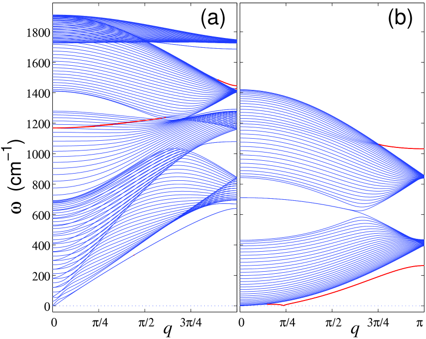
Figure 3: Structure of $3N_{e}$ dispersion curves for zigzag graphene nanoribbon (C₆₄H₂)_∞ for (a) in-plane and (b) out-of-plain vibrations. The thick red curves correspond to oscillations localized at the nanoribbon edges.

IV Graphene frequency spectrum

Let us consider a wide nanoribbon (C₆₄H₂)_∞ (the nanoribbon width $D=68.79$Å, the period $a=2.412$Å, the number of atoms in unit cell $N_{e}=66$) to find the frequency spectrum of graphene sheet. Figure 3 shows the $3N_{e}$ dispersion curves of the nanoribbon. The plane structure of the nanoribbon allows to divide its vibrations into two classes: in-plane vibrations, when the atoms are always stayed in the plane of the nanoribbon and out-of-plane vibrations when the atoms are shifted orthogonal to the plane. Two third of the branches corresponds to the atom vibrations in the $xy$ plane of the nanoribbon (in-plane vibrations), whereas only one third corresponds to the vibrations orthogonal to the plane (out-of-plane vibrations), when the atoms are shifted along the axes $z$.

The nanoribbon frequency spectrum consists of two intervals $[0,1911]$ and $[3086.6,3099.2]$ cm^-1 (the second high-frequency interval corresponds to the edge vibrations of the valence bonds C–H). Discarding frequencies of the edge vibrations from the Figure 3, we can conclude that graphene sheet spectrum consists of the one frequency interval $[0,\omega_{m}]$ with the maximum frequency $\omega_{m}=1911$ cm^-1. Spectrum of out-of-plane vibrations also consists of the one frequency interval $[0,\omega_{o}]$ with the maximum frequency $\omega_{o}=1420$ cm^-1.

The frequency spectrum of graphene sheet has been studied theoretically and experimentally in pm57 ; pm58 ; pm59 ; pm60 . The maximum frequency of in-plane vibrations is $\omega_{m}=1600$ cm^-1, the maximum frequency of out-of-plane vibrations is $\omega_{o}=868$ cm^-1. Thus, the graphene frequency spectrum calculated by the COMPASS force field does not coincide with experimental valuations. The frequency spectrum of in-plane vibrations is 1.2 times more and the frequency spectrum of out-of-plane vibrations is 1.6 times more than experimental valuations, i.e. the bending stiffness of the nanoribbon is 2.5 times more.

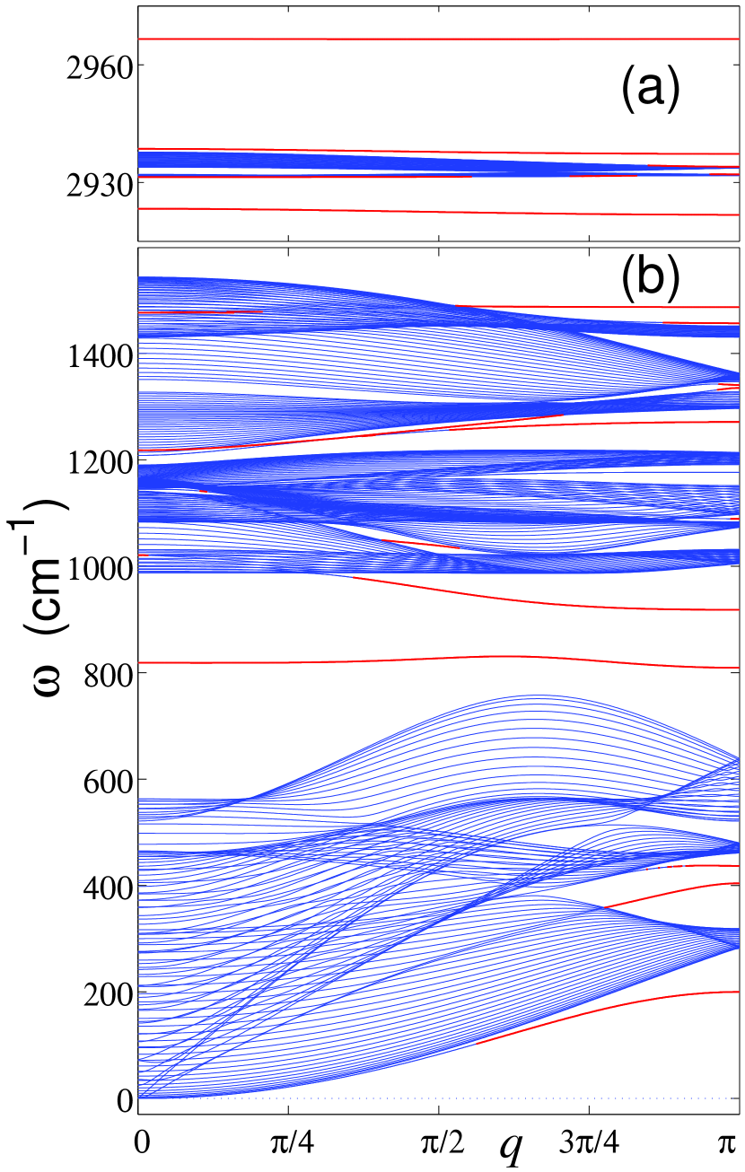
Figure 4: Structure of $3N_{e}$ dispersion curves for zigzag graphane nanoribbon (C₆₄H₆₆)_∞. The thick red curves correspond to oscillations localized at the nanoribbon edges.

V Graphane and fluorographene frequency spectrum

Let us consider a wide nanoribbon (C₆₄H₆₆)_∞ (nanoribbon width $D=68.4$Å, period $a=2.522$Å, number atoms in unit cell $N_{e}=130$) to find the frequency spectrum of graphane sheet. Figure 4 shows the dispersion curves of the nanoribbon. As can be seen from the figure, the nanoribbon frequency spectrum consists of three intervals: low-frequency interval $[0,757.8]$, middle-frequency interval $[987.5,1543.6]$ and narrowhigh-frequency interval $[2921.8,2966.6]$ cm^-1. On average, carbon atoms account for 79.5% of the vibration energy in the first frequency interval, for 48.1% in the second frequency interval and only for 8.4% in the third. It enables us to say that the low-frequency spectrum corresponds to the vibrations, in which the valence bond C–H and the valence angles C–C–H remain nearly unchanged, the middle interval corresponds to the vibrations, in which the valence corners C–C–H begin to take part in the vibration, and the third interval corresponds to the vibrations of the hard valence bonds C–H (the number of such modes always coincide with the number of hydrogen atoms).

Since we have considered as sufficiently broad nanoribbon, the analysis of its dispersal curves suggests that the frequency spectrum of linear vibrations of the endless graphene sheet (CH)_∞ consists of three continuous intervals $[0,756]$, $[987,1544]$ and $[2922,2967]$ cm^-1. Thus, the graphene sheet has two gaps in the frequency spectrum: narrow low-frequency $[756,987]$ and widehigh-frequency $[1544,2922]$ cm^-1. Such structure of the frequency spectrum is in good agreement with the results of first-principles calculations. Quantum calculations suggest the high-frequency spectrum intervals$[0,806]$, $[950,1350]$ and $[2733,2783]$ cm^-1 pm61 .

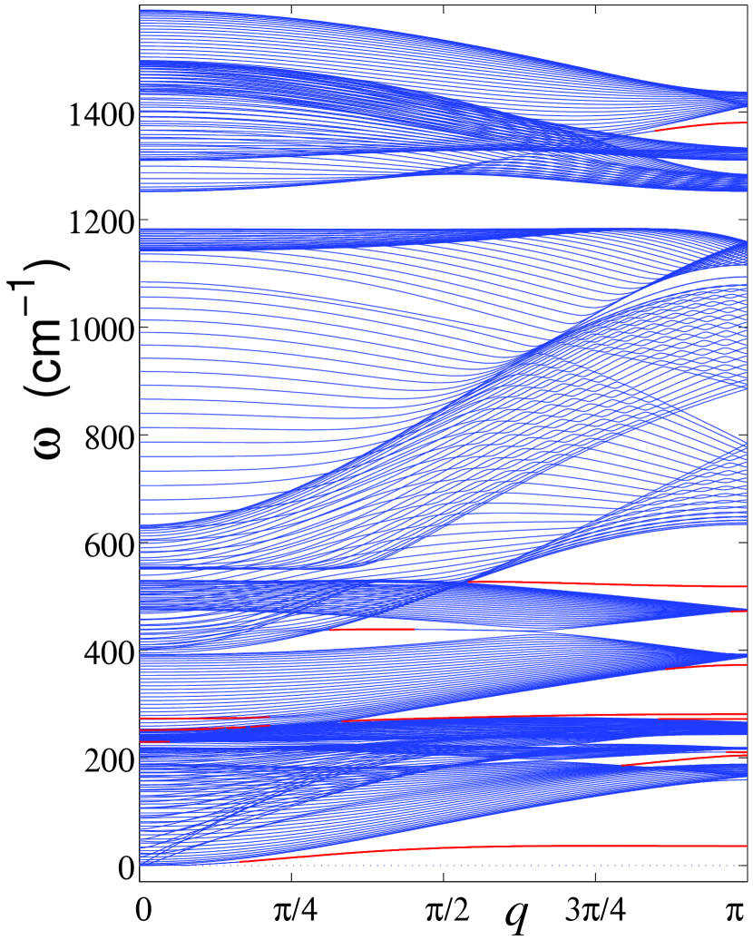
Figure 5: Structure of $3N_{e}$ dispersion curves for zigzag graphene fluoride nanoribbon (C₆₄F₆₆)_∞. The thick red curves correspond to oscillations localized at the nanoribbon edges.

If the hydrogen atoms H change to the heavier deuterium atoms D, the three-zoned structure of the frequency spectrum will remain, but all the frequencies will shift down. The frequency spectrum of graphene sheet (CD)_∞ also consists of three intervals $[0,620]$, $[813,1503]$, $[2130,2200]$ cm^-1 (the high-frequency interval most strongly shifts down). The stronger increase in the weight of the connected atoms, the change of hydrogen atoms for fluorine atoms, causes the stronger frequency shift and the closure of the gaps.

Figure 5 shows the dispersion curves for fluorographene nanoribbon (C₆₄F₆₆)_∞. The figure clearly shows that the nanoribbon frequency spectrum of linear vibrations consists of two intervals: $[0,1183.6]$ and$[1252.0,1589.3]$ cm^-1. The analysis of the dispersion curves suggests that the frequency spectrum of linear vibrations of the endless fluorographene sheet (CF)_∞ consists of two continuous intervals $[0,1184]$ and$[1252,1589]$ cm^-1 with the narrow gap between them. Such structure of the frequency spectrum is also in good agreement with the results of quantum chemical calculations pm61 . Quantum calculations suggest the frequency spectrum intervals $[0,1039]$ and$[1106,1312]$ cm^-1.

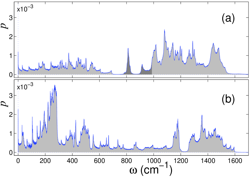
Figure 6: Density of states $p(\omega)$ of atom vibrations in (a) graphane nanoribbon (C₁₂H₁₄)₉₉C₁₀H₂₂ (darker color corresponds to frequency region of the gap edge modes) and (b) graphene fluoride nanoribbon (C₁₂F₁₄)₉₉C₁₀F₂₂ for temperature $T=300$K. The density of states is normalized by the condition $\int_{0}^{\infty}p(\omega)d\omega=1$.

The structure of the frequency spectrum can be obtained also from the analysis of the frequency spectrum density of atomic thermal vibrations of finite length nanoribbon. Let us consider the graphane nanoribbon (C₁₂H₁₄)₉₉C₁₀H₂₂ with size $25.09\times 1.17$ nm², consisted of $N=100$ unit cells.

The dynamics of the thermalized nanoribbon is described by the system of Langevin equations

$$M_{n,k}\ddot{\bf u}_{n,k}=-\frac{\partial H}{\partial{\bf u}_{n,k}}-\Gamma M_{n,k}+\Xi_{n,k},$$ (10)

$$n=1,2,...,N,~{}~{}k=1,2,...,N_{e},$$

where $H$ – Hamiltonian of the nanoribbon, created by the COMPASS force field, ${\bf u}_{n,k}=(u_{n,k,1},u_{n,k,2},u_{n,k,3})$ – 3D coordinate vector of atom $(n,k)$, $M_{n,k}$ – mass of this atom, $\Gamma=1/t_{r}$ – damping coefficient (relaxation time $t_{r}=0.4$ ps). Normally distributed random forces $\Xi_{n,k}=(\xi_{n,k,1},\xi_{n,k,2},\xi_{n,k,3})$ normalized by conditions

$$\langle\xi_{n,k,i}(t_{1})\xi_{m,l,j}(t_{2})\rangle=2M_{n,k}\Gamma k_{B}T\delta_{nm}\delta_{kl}\delta_{ij}\delta(t_{1}-t_{2}),$$

where $k_{B}$ – Boltzmann’s constant, $T$ – thermostat temperature.

The system of equations of motion (10) was integrated numerically during the time $t=10$ ps (the stationary state of the plane nanoribbon serves as a starting point). During this time, the nanoribbon and the thermostat came to balance. Then its interaction with the thermostat was switched off and the dynamics of isolated thermalized nanoribbon was considered. The density of the frequency spectrum of atomic vibrations $p(\omega)$ was calculated via fast Fourier transform.

The density of the frequency spectrum of atomic vibrations of the graphane and fluorographene nanoribbons at $T=300$ K is presented in Fig. 6. The figure clearly shows that the profile of density $p(\omega)$ coincides well with the forms of the dispersal curves. The low-frequency gap is clearly visible for the graphane nanoribbon, and the narrow gap in the frequency spectrum is clearly visible for the fluorographene nanoribbon.

VI Corrections of the COMPASS force field for graphene sheet

The simulation shows that the COMPASS force field does not describe well the frequency spectrum of graphene sheet. The frequency spectrum of out-of-plane vibrations differs strongly from the experimental values.

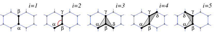
Figure 7: Configurations containing up to $i$-th nearest-neighbor interactions in graphene sheet.

The potential energy of the graphene sheet depends on variations in bond length, bond angles, and dihedral angles between the planes formed by three neighboring carbon atoms and it can be written in the form

$$E=\sum_{\Omega_{1}}V_{1}+\sum_{\Omega_{2}}V_{2}+\sum_{\Omega_{3}}V_{3}+\sum_{\Omega_{4}}V_{4}+\sum_{\Omega_{5}}V_{5},$$ (11)

where $\Omega_{i}$, with $i=1,2,3,4,5$, are the sets of configurations including up to nearest-neighbor interactions. Owing to a large redundancy, the sets only need to contain configurations of the atoms shown in Fig. 7, including their rotated and mirrored versions. The potential$V_{1}({\bf u}_{\alpha},{\bf u}_{\beta})$ describes the deformation energy due to a direct interaction between pairs of atoms with the indexes $\alpha$ and $\beta$. The potential $V_{2}({\bf u}_{\alpha},{\bf u}_{\beta},{\bf u}_{\gamma})$ describes the deformation energy of the angle between the valent bonds ${\bf u}_{\alpha}{\bf u}_{\beta}$ and ${\bf u}_{\beta}{\bf u}_{\gamma}$.

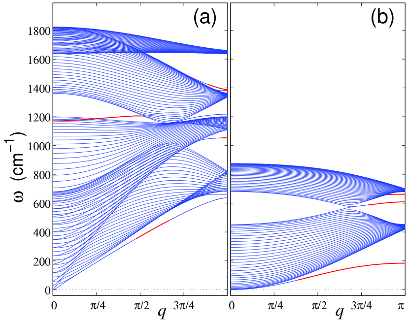
Figure 8: Structure of $3N_{e}$ dispersion curves for zigzag graphene nanoribbon (C₆₄H₂)_∞ for (a) in-plane and (b) out-of-plain vibrations. The thick red curves correspond to oscillations localized at the nanoribbon edges. The force field COMPASS with correction of parameters (12) was used.

Potentials $V_{i}({\bf u}_{\alpha},{\bf u}_{\beta},{\bf u}_{\gamma},{\bf u}_{\delta})$, $i=3,4,5$, describes the deformation energy associated with a change of the effective angle between the planes ${\bf u}_{\alpha}{\bf u}_{\beta}{\bf u}_{\gamma}$ and ${\bf u}_{\beta}{\bf u}_{\gamma}{\bf u}_{\alpha}$ as shown in Fig. 7.

In the COMPASS force field the first potential $V_{1}=k_{b,2}(b-b_{0})^{2}+k_{b,3}(b-b_{0})^{3}+k_{b,4}(b-b_{0})^{4}$ describes the deformations of valence bonds, the second potential $V_{2}=k_{\theta,2}(\theta-\theta_{0})^{2}+k_{\theta,3}(\theta-\theta_{0})^{3}+k_{\theta,4}(\theta-\theta_{0})^{4}$ – the deformations of valence angles, the third potential $V_{3}(\chi)=k_{\chi}\chi^{2}$ – out-of-plane deformations. The potentials of dihedral angles $V_{4}$ and $V_{5}$ are described by a single potential of the torsional angle $V_{t}(\phi)=k_{\phi,1}(1-\cos\phi)+k_{\phi,2}(1-\cos 2\phi)+k_{\phi,3}(1-\cos 3\phi)$.

The specific value of the parameter $\kappa_{\chi}=5.7537$ kcal/mol can be found from the frequency spectrum of small-amplitude oscillations of a sheet of graphite sav1 . For the potentials of dihedral angles $V_{4}=c_{4}(\phi-\pi)^{2}$ and $V_{5}=c_{5}\phi^{2}$ according to the results of Ref. sav2 coefficient $c_{4}$ is close to $k_{\chi}$, whereas $c_{5}\ll c_{4}$ ($|c_{5}/c_{4}|<1/20$). So for the second derivative of the torsion potential we have

$$V_{t}^{\prime\prime}(0) = k_{\phi,1}+4k_{\phi,2}=V_{5}^{\prime\prime}(0)=0,$$

$$V_{t}^{\prime\prime}(\pi) = -k_{\phi,1}+4k_{\phi,2}=V_{4}^{\prime\prime}(0)=2c_{4}=2k_{\chi},$$

therefore coefficients $k_{\phi,2}=k_{\chi}/4=1.4384$ kcal/mol, $k_{\phi,1}=-4k_{\phi,2}=-5.7537$ kcal/mol.

Now let us consider the COMPASS force field with the new parameters values

$$k_{\chi}=-k_{\phi,1}=5.7537,~{}~{}k_{\phi,2}=1.4384\mbox{kcal/mol}.$$ (12)

Since all the parameters for the off-diagonal interactions bond/torsion, angle/torsion and angle/angle/torsion have become undefined after such a modification, remove them away from the force field. Then we find the frequency value of the graphene sheet via that modification of the force field.

Figure 8 shows the dispersal curves of the graphene nanoribbon (C₆₄H₂)_∞ calculated via the modified COMPASS force field. From figure, we can conclude that now the spectrum of the graphene sheet consists of the frequency interval of in-plane vibrations $[0,1823]$ and the frequency interval of out-of-plane vibrations $[0,876]$ cm^-1, that is in good agreement with the results described in pm57 ; pm58 ; pm59 ; pm60 . Thus, modification (12) of the COMPASS force field allows to take into account the flexural mobility of graphene sheet (the initial set of parameters led to an over estimation of the bending stiffness)

VII Conclusion

The study shows that the COMPASS force field allows to describe with good accuracy the frequency spectrum of atomic vibrations of graphane and fluorographene sheets, whose honeycomb hexagonal lattice is formed by sp³ valence bands. On the other hand, the force field doesn’t describe very well the frequency spectrum of graphene sheet, whose planar hexagonal lattice is formed by sp² valence bands. In that case the frequency spectrum of out-of-plane vibrations differs greatly from the experimental data (bending stiffness of a graphene sheet is strongly overestimated). The correction (12) of parameters of out-of-plane and torsional potentials of the force field was made, and that allows to achieve the coincidence of vibration frequency with experimental data. After such corrections the COMPASS force field can be used to describe the dynamics of flat graphene sheets and carbon nanotubes.

References

- (1) Novoselov KS, Geim AK, Morozov SV, Jiang D, Zhang Y, Dubonos SV, Grigorieva IV, Firsov AA (2004) Electric field effect in atomically thin carbon films. Science 306:666-669. https://doi.org/10.1126/science.1102896
- (2) Mohan VB, Lau K, Hui D, Bhattacharyya D (2018) Graphene-based materials and their composites: A review on production, applications and product limitations. Composites B 142:200-220. https://doi.org/10.1016/j.compositesb.2018.01.013
- (3) Akinwande D, Brennan CJ, Bunch JS et al (2017) A review on mechanics and mechanical properties of 2D materials-Graphene and beyond. Extreme Mechanics Letters 13:42-77. http://dx.doi.org/10.1016/j.eml.2017.01.008
- (4) Harik V (2018) Mechanics of Carbon Nanotubes. Fundamentals, Modelling and Safety. Academic Press. https://doi.org/10.1016/C2016-0-00799-4
- (5) Feng W, Long P, Feng Y, Li Y (2016) Two-Dimensional Fluorinated Graphene: Synthesis, Structures, Properties and Applications. Adv. Sci. 3, 1500413. https://doi.org/10.1002/advs.201500413
- (6) Chen T, Cheung R (2016) Mechanical properties of graphene. In: Aliofkhazraei M, Ali N, Milne WI, Ozkan CS, Mitura S, Gervasoni JL (eds.) Graphene Science Handbook: Mechanical and Chemical Properties. CRC Press, London. pp. 3-15
- (7) Bhimanapati GR, Lin Z, Meunieret V et al (2015) Recent advances in two-dimensional materials beyond graphene. ACS Nano 9:11509-115399. https://doi.org/10.1021/acsnano.5b05556
- (8) Cao G (2014) Atomistic Studies of Mechanical Properties of Graphene. Review. Polymers 6:2404-2432. https://doi.org/10.3390/polym6092404
- (9) Li X, Tao L, Chen Z, Fang H, Li X, Wang X, Xu J-B, Zhu H (2017) Graphene and related two-dimensional materials: Structure-property relationships for electronics and optoelectronics. Appl. Phys. Rev. 4, 021306 (2017). http://dx.doi.org/10.1063/1.4983646
- (10) Geim AK, Novoselov KS (2007) The rise of graphene. Nat. Mater. 6:183-191. https://doi.org/10.1038/nmat1849
- (11) Brar VW, Sherrott MC, Jariwala D (2018) Emerging photonic architectures in two-dimensional opto-electronics. Chem. Soc. Rev. 47:6824-6844. https://doi.org/10.1039/c8cs00206a
- (12) Khan ME, Khan MM, Cho MH (2018) Recent Progress of Metal-Graphene Nanostructures in Photocatalysis. Nanoscale 10: 9427-9440. https://doi.org/10.1039/C8NR03500H
- (13) Ferrari AC, Bonaccorso F, Fal’ko V, et al (2015) Science and technology roadmap for graphene, related two-dimensional crystals, and hybrid systems. Nanoscale 7:4598-5062. https://doi.org/10.1039/c4nr01600a
- (14) Xiang Q, Cheng B, Yu J (2015) Graphene-Based Photocatalysts for Solar-Fuel Generation. Angew. Chem., Int. Ed. 54:11350-11366. https://doi.org/10.1002/anie.201411096
- (15) Ryu J, Lee E, Lee K, Jang J (2015) A Graphene Quantum Dots Based Fluorescent Sensor for Anthrax Biomarker Detection and Its Size Dependence. J. Mater. Chem. B 3:4865-4870 https://doi.org/10.1039/C5TB00585J
- (16) Soldano C, Mahmood A, Dujardin E (2010) Production, properties and potential of graphene. Carbon 48:2127-2150. https://doi.org/10.1016/j.carbon.2010.01.058
- (17) Li X, Zhi L (2018) Graphene hybridization for energy storage applications. Chem. Soc. Rev. 47:3189-3216. https://doi.org/10.1039/C7CS00871F
- (18) Siahlo AI, Poklonski NA, Lebedev AV, Lebedeva IV, Popov AM, Vyrko SA, Knizhnik AA, Lozovik YE (2018) Structure and energetics of carbon, hexagonal boron nitride, and carbon/hexagonal boron nitride single-layer and bilayer nanoscrolls. Phys. Rev. Mater. 2, 036001. https://doi.org/10.1103/PhysRevMaterials.2.036001
- (19) Azadmanjiri J, Srivastava VK, Kumar P, Nikzad M, Wang J, Yu A (2018) Two- and three-dimensional graphene-based hybrid composites for advanced energy storage and conversion devices. J. Mater. Chem. A 6, 702-734. https://doi.org/10.1039/C7TA08748A
- (20) Sunnardianto GK, Maruyama I, Kusakabe K (2017) Storing-hydrogen processes on graphene activated by atomic-vacancies. International Journal of Hydrogen Energy 42:23691-23697. https://doi.org/10.1016/j.ijhydene.2017.01.115
- (21) Stankovich S, Dikin DA, Dommett GHB, Kohlhaas KM, Zimney KM, Stach EA, Piner RD, Nguyen ST, Ruoff RS (2006) Graphene-based composite materials. Nature 442:282-286. https://doi.org/10.1038/nature04969
- (22) Tan KH, Sattari S, Donskyi IS, Cuellar-Camacho JL, Cheng C, Schwibbert K, Lippitz A, Unger WES, Gorbushina A, Adeli M, Haag R (2018) Functionalized 2D nanomaterials with switchable binding to investigate graphene-bacteria interactions. Nanoscale 10:9525-9537. https://doi.org/10.1039/c8nr01347k
- (23) Cheng C, Li S, Thomas A, Kotov NA, Haag R (2017) Functional Graphene Nanomaterials Based Architectures: Biointeractions, Fabrications, and Emerging Biological Applications. Chem. Rev. 117:1826-9537. https://doi.org/10.1039/c8nr01347k
- (24) Brenner DW (1990) Empirical potential for hydrocarbons for use in simulating the chemical vapor deposition of diamond films. Phys. Rev. B 42:9458-9471. https://doi.org/10.1103/PhysRevB.42.9458
- (25) Stuart SJ, Tutein AB, Harrison JA (2000) A reactive potential for hydrocarbons with intermolecular interactions. J. Chem. Phys. 112:6472. https://doi.org/10.1063/1.481208
- (26) Brenner DW, Shenderova OA, Harrison JA, Stuart SJ, Ni B, Sinnott SB (2002) A second-generation reactive empirical bond order (REBO) potential energy expressi2on for hydrocarbons. J. Phys.: Condens. Matter 14:783-802. https://doi.org/10.1088/0953-8984/14/4/312
- (27) Lindsay L, Briodo DA (2010) Optimized Tersoff and Brenner empirical potential parameters for lattice dynamics and phonon thermal transport in carbon nanotubes and graphene. Phys. Rev. B 81:205441. https://doi.org/10.1103/PhysRevB.81.205441
- (28) Senftle TP, Hong S, Islam MM and et al (2016) The ReaxFF reactive force-field: Development, applications and future Directions. npj Comput. Mater. 2:15011 (2016). https://doi.org/10.1038/npjcompumats.2015.11
- (29) Los JH, Ghiringhelli LM, Meijer EJ, Fasolino A (2005) Improved long-rangereactive bond-order potential for carbon. I. Construction. Phys Rev. B 72, 214102. https://doi.org/10.1103/PhysRevB.72.214102
- (30) Zhou XW, Ward DK, Foster ME (2015) An analytical bond-order potential for carbon. J Comput Chem. 36:11719-1735. https://doi.org/10.1002/jcc.23949
- (31) Marks NA (2001) Generalizing the environment-dependent interaction potential for carbon. Phys Rev B. 63, 035401. https://doi.org/10.1103/PhysRevB.63.035401
- (32) Uddin J, Baskes MI, Srinivasan SG, Cundari TR, Wilson AK (2010) Modified embedded atom method study of the mechanical properties of carbon nanotube reinforced nickel composites. Phys Rev B. 81, 104103. https://doi.org/10.1103/PhysRevB.81.104103
- (33) Mayo SL, Olafson BD, Goddard III WA (1990) DREIDING: a generic force field for molecular simulations. J. Phys. Chem. 94:8897-8909. https://doi.org/10.1021/j100389a010
- (34) Tserpes KI, Papanikos P (2014) Finite element modeling of the tensile behavior of carbon nanotubes, graphene and their composites. In: Tserpes KI, Silvestre N (eds.) Springer Series in Materials Science, vol. 188: Modeling of Carbon Nanotubes, Graphene and their Composites, Springer International Publishing, Champp. 303-329
- (35) Kalosakas G, Lathiotakis NN, Galiotis C, Papagelis K (2013) In-plane force fields and elastic properties of graphene. J. APP. Phys. 113, 134307. https://doi.org/10.1063/1.4798384
- (36) Fthenakis ZG, Kalosakas G, Chatzidakis GD, Galiotis C, Papagelis K, Lathiotakis NN (2017) Atomistic potential for graphene and other sp2 carbon systems. Phys. Chem. Chem. Phys. 19, 30925-30932. https://doi.org/10.1039/c7cp06362h
- (37) Chatzidakis GD, Kalosakas G, Fthenakis ZG, Lathiotakis NN (2018) A torsional potential for graphene derived from fitting to DFT results. Eur. Phys. J. B 91, 11. https://doi.org/10.1140/epjb/e2017-80444-5
- (38) Zalizniak VE, Zolotov OA (2017) Efficient embedded atom method interatomic potential for graphite and carbon nanostructures. Molecular Simulation 43:1480-1484. http://dx.doi.org/10.1080/08927022.2017.1324957
- (39) Korobeynikov SN, Alyokhin VV, Babichev AV (2018) Simulation of mechanical parameters of graphene using the DREIDING force field. Acta Mech 229:2343-2378. https://doi.org/10.1007/s00707-018-2115-5
- (40) Sun H (1998) COMPASS: An ab initio force-field optimized for condensed-phase applications – Overview with details on alkane and benzene compounds. J. Phys. Chem. B 102:7338-7364. https://doi.org/10.1021/jp980939v
- (41) Sun H, Jin Z, Yang C, Akkermans RL, Robertson SH, Spenley NA, Miller S, Todd SM (2016) COMPASS II: extended coverage for polymer and druglike molecule databases. J. Mol. Model. 22:47. https://doi.org/10.1007/s00894-016-2909-0
- (42) Cao GX, Chen X (2007) The effects of chirality and boundary conditions on the mechanical properties of single-walled carbon nanotubes. Int. J. Solids Struct. 44:5447-5465. https://doi.org/10.1016/j.ijsolstr.2007.01.005
- (43) Zhang J, He X, Yang L, Wu G, Sha J, Hou C, Yin C, Pan A, Li Z, Liu Y (2013) Effect of Tensile Strain on Thermal Conductivity in Monolayer Graphene Nanoribbons: A Molecular Dynamics Study. Sensors 13:9388-9395. https://doi.org/10.3390/s130709388
- (44) Zhou LX, Wang YG, Cao GX (2013) Elastic properties of monolayer graphene with different chiralities. J. Phys. Condens. Mater. 25, 125302. https://doi.org/10.1088/0953-8984/25/12/125302
- (45) Shen X, Lin XY, Yousefi N, Jia JJ, Kim JK (2014) Wrinkling in graphene sheets and graphene oxide papers. Carbon 66:84-92. https://doi.org/10.1016/j.carbon.2013.08.046
- (46) Melro LS, Pyrz R, Jensen LR (2016) A molecular dynamics study on the interaction between epoxy and functionalized graphene sheets. Materials Science and Engineering 139, 012036. https://doi.org/10.1088/1757-899X/139/1/012036
- (47) Savin AV, Mazo MA (2017) Molecular Dynamics Simulation of Two-Sided Chemical Modification of Carbon Nanoribbons on a Solid Substrate. Dokl. Phys. Chem. 473:37-40. https://doi.org/10.1134/S0012501617030022
- (48) A.V. Savin (2018) Edge Vibrations of Graphane Nanoribbons. Phys. Solid State 60:1046-1053. https://doi.org/10.1134/S1063783418050281
- (49) Savin AV, Sakovich RA, Mazo MA (2018) Using spiral chain models for study of nanoscroll structures. Phys. Rev. B 97, 165436. https://doi.org/10.1103/PhysRevB.97.165436
- (50) Sluiter MHF, Kawazoe Y (2003) Cluster expansion method for adsorption: Application to hydrogen chemisorption on graphene. Phys. Rev. B 68, 085410. https://doi.org/10.1103/PhysRevB.68.085410
- (51) Sofo JO, Chaudhari AS, Barber GD (2007) Graphane: A two-dimensional hydrocarbon. Phys. Rev. B 75, 153401. https://doi.org/10.1103/PhysRevB.75.153401
- (52) Elias DC, Nair RR, Mohiuddin TMG et al (2009) Control of Graphene’s Properties by Reversible Hydrogenation: Evidence for Graphane. Science 323:610-613. https://doi.org/10.1126/science.1167130
- (53) Samarakoon D.K., Wang X-Q (2009) Chair and Twist-Boat Membranes in Hydrogenated Graphene. ACS Nano 3:4017-4022. https://doi.org/10.1021/nn901317d
- (54) Yang YE, Yang Y-R, Yan X-H (2012) Universal optical properties of graphane nanoribbons: A first-principles study Physica E 44:1406-1409. https://doi.org/10.1016/j.physe.2012.03.002
- (55) Peng Q, Dearden AK, Crean J, Han L, Liu S, Wen X, De S (2014) New materials graphyne, graphdiyne, graphone, and graphane: review of properties, synthesis, and application in nanotechnology. Nanotechnol. Sci. App. 7:1-29. https://doi.org/10.2147/NSA.S40324
- (56) Sahin H, Leenaerts O, Singh SK, Peeters FM (2015) Graphane. WIREs Comput Mol Sci 5:255-272. https://doi.org/10.1002/wcms.1216
- (57) Al-Jishi R, Dresselhaus G (1982) Lattice-dynamical model for graphite. Phys. Rev. B 26:4514-4522. https://doi.org/10.1103/PhysRevB.26.4514
- (58) Aizawa T, Souda R, Otani S, Ishizawa Y, Oshima C (1990) Bond softening in monolayer graphite formed on transition-metal carbide surfaces. Phys. Rev. B 42:11469-11478. https://doi.org/10.1103/PhysRevB.42.11469
- (59) Maultzsch J, Reich S, Thomsen C, Requardt H, Ordejon P (2004) Phonon Dispersion in Graphite. Phys. Rev. Lett. 92, 075501. https://doi.org/10.1103/PhysRevLett.92.075501
- (60) Mohr M, Maultzsch J, Dobardzic E et al (2007) Phonon dispersion of graphite by inelastic x-ray scattering. Phys. Rev. B 76, 035439. https://doi.org/10.1103/PhysRevB.76.035439
- (61) Peelaers H, Hernandez-Nieves AD, Leenaerts O, Partoens B, Peeters FM Vibrational properties of graphene fluoride and graphane. Appl. Phys. Lett. 98, 051914. https://doi.org/10.1063/1.3551712
- (62) Savin AV, Kivshar YuS (2008) Discrete breathers in carbon nanotubes. Europhys. Letters 82, 66002. https://doi.org/10.1209/0295-5075/82/66002
- (63) Gunlycke D, Lawler HM, White CT (2008) Lattice vibrations in single-wall carbon nanotubes. Phys. Rev B 77, 014303. https://doi.org/10.1103/PhysRevB.77.014303