Fast flux control of 3D transmon qubits using a magnetic hose

Abstract

Fast magnetic flux control is a crucial ingredient for circuit quantum electrodynamics (cQED) systems. So far it has been a challenge to implement this technology with the high coherence 3D cQED architecture. In this paper we control the magnetic field inside a superconducting waveguide cavity using a magnetic hose, which allows fast flux control of 3D transmon qubits on time scales $<$100 ns. The hose is designed as an effective microwave filter to not compromise the energy relaxation time of the qubit. The magnetic hose is a promising tool for fast magnetic flux control in various platforms intended for quantum information processing and quantum optics.

In many quantum systems used for quantum information processing, quantum optics and quantum enhanced measurements, magnetic fields are essential to mediate interactions or tune parameters. Taylor et al. (2008); Chin et al. (2010); Warring et al. (2013) For individual quantum systems like qubits the typical wish-list is a combination of large field strength, the ability to change the field rapidly and apply it only locally while at the same time not introduce additional decoherence channels. Very often it is hard for experiments to simultaneously meet these criteria as e.g. fast switching times are limited by eddy or super-currents introduced by the metallic boundaries protecting the quantum system from decoherence.

One of the most promising platforms for realising a quantum computer are superconducting qubits. Magnetic fields play an important role in this architecture to tune the frequency of individual qubits, change the coupling between pairs of qubits Chen et al. (2014) as well as apply parametric drives for quantum limited amplifiers Yamamoto et al. (2008); Mutus et al. (2013) and novel coupling schemes Chen et al. (2014); Caldwell et al. (2018). So called flux bias lines DiCarlo et al. (2009) are widely used in planar superconducting qubit architectures but so far it has proven to be difficult to implement a similar technology in a 3D architecture Reshitnyk et al. (2016); Kong et al. (2015). The problems in this architecture arise on one hand due to the difficulty of applying magnetic fields through a superconducting wall and on the other hand achieving fast tunability without compromising the qubit lifetime.

In this paper we demonstrate magnetic field control inside a superconducting waveguide cavity using a magnetic hose Navau et al. (2014). The hose is designed as an effective microwave filter to not compromise the energy relaxation time of the qubit and allow for fast flux control of 3D transmon qubits on time scales $<$ 100 ns. This technology can be broadly used to guide magnetic fields from an external coil to a quantum system sensitive to magnetic flux placed inside a metal or superconducting structure or even to mediate magnetic interaction between two quantum systems.

Figure 1: (a) Photograph of one half of a rectangular waveguide cavity with two transmon qubits fabricated on sapphire pieces separated by a distance of about 3 mm. The cavity has a hole in the middle of the back wall to attach a magnetic hose. On the back side of the cavity, not visible in the picture, a copper clamp is used to fix and thermalize the hose. (b) Schematic of the setup highlighting the hose, with a coil (yellow) on the external side and a qubit (black structures on the two pieces of sapphire (green)) on the other. Inset: Cross section of the hose, showing the shell structure (grey = ferromagnetic layers, light blue = superconducting layers) with a vertical cut.

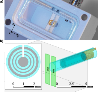
Our system, illustrated in Fig. 1, is constituted by two transmon qubits separated by a distance of about 3 mm, fabricated on two different sapphire pieces. Both sapphire pieces are placed in a rectangular aluminium cavity, which is adapted to the hose by drilling a hole in the middle of one of the faces.

Figure 2: Top (a) and side (b) view of the setup, showing the magnetic field’s x-component on a logarithmic scale. The grey part below ($x<0$) depicts the cavity wall, the thin light blue surfaces indicate the superconducting shells of the magnetic hose, where the magnetic field is zero. The qubits’ positions are represented by black lines on green squares, which indicate the sapphire chips. The magnetic field distribution is calculated by a finite element simulation in the case of static magnetic fields. In this case the setup simplifies to its magnetic properties only and the superconductor and ferromagnet are well approximated by materials with $\mu_{r}=10^{-4}$ and $\mu_{r}=10^{4}$, respectively sidenote1 . The source of magnetic field is a solenoid placed at the entrance of the hose (not visible). Its dimensions and magnetisation correspond to the coil used in the experiment when a current of 10 mA is fed. The magnetic field is 3.55 nT at the central and 0.75 nT at the side qubit.

The magnetic hose consists of a set of concentric cylindrical layers. Half of the layers are made of ferromagnetic material (with large magnetic permeability) and the other half of superconducting material (with a permeability effectively $\mu_{r}\rightarrow 0$). These two types of layers are alternated forming a magnetic metamaterial structure. Such structure exhibits an extremely anisotropic effective magnetic permeability, with very large permeability along the axial direction of the hose, $\mu_{r}^{||}\rightarrow\infty$, and a very small permeability in the (radial) perpendicular direction, $\mu_{r}^{\perp}\rightarrow 0$. Intuitively, the ferromagnetic layers provide large permeability components in all directions, but the interlayered superconducting layers shield any radial magnetic field component. The design of this metamaterial structure Navau et al. (2014), which results from concepts in transformation optics Pendry et al. (2006); Chen et al. (2010), allows to transfer static magnetic fields over long distances. To that effect, a dense structure of alternating layers is essential for preventing losses and enhancing the transport.

Following this idea, we built a hose consisting of four ferromagnetic layers made of mu-metal and four superconducting layers made of aluminum. The seven innermost layers are 10 mm long and the outermost aluminium shell is 20 mm long. This external superconducting shell pushes the magnetic field further into the cavity. Additionally, we introduce a cut through all layers along the magnetic hose (see Fig 1b). All aluminium shells have a thickness of 200 $\mu$m, the two innermost mu-metal shells are 100 $\mu$m thick and the outermost mu-metal shell is 200 $\mu$m thick. All shells are wrapped around a 1 mm thick central mu-metal wire. The coil at one end of the hose has 10 turns, a diameter of 3 mm, and a length of 4 mm, resulting in a self inductance of 126 nH in free space. When the coil is attached to the hose, the self inductance is reduced to 81 nH due to the outermost superconducting shell surrounding it.

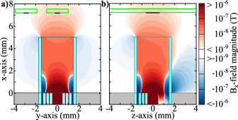
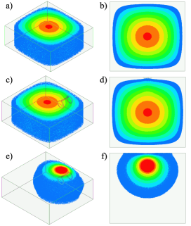
The question arises if one can use such a magnetic hose for transporting a magnetic flux pulse generated outside to the inside of a superconducting cavity and locally act on a flux sensitive qubit. A magneto-static simulation shows that the magnetic hose is able to route magnetic field through a hole into a superconducting box as depicted in Fig. 2. At first glance this seems to contradict the concept of flux quantization, which prevents any net magnetic flux from passing through the area of a closed superconducting ring that has been cooled in absence of magnetic field. However, the magnetic field is not only guided into the cavity, it is also routed back to the outside through the same hole. As a result, the total magnetic flux through the hole is always zero and flux quantization is fulfilled. Implications of flux quantization also extend to the superconducting layers forming the hose itself. For this reason, a magnetic hose can transport magnetic field only if all superconducting layers are cut along their length, preventing super-currents to flow in closed circles. Since ferromagnetic layers also have some electrical conductivity, the cut is also extended to them in order to minimize circular eddy currents (see the inset of Fig. 1b). As a result, not only static but even fast alternating magnetic fields can be transported.

Despite the magnetic hose opening a link for magnetic fields through the cavity wall, it is designed to prevent electromagnetic waves inside the cavity from leaking out to the environment. The elongated part of the outermost shell acts as a $\lambda/4$ resonator with a resonance frequency around 10 GHz. Any electro-magnetic wave below this resonance is reflected and does not reach the ferromagnetic core of the hose. The cut introduced in the hose layers acts as a rectangular waveguide with a cut-off frequency of more than 100 Ghz. Thus, the magnetic hose does not provide any additional loss channel for microwaves at the qubit and cavity frequencies, which was verified by finite element simulations. In summary, a magnetic hose acts as a filter between the coil and the qubit and, due to its shape, the transported magnetic field is applied very locally.

Figure 3: Detuning from the maximum transition frequency of both qubits as a function of the applied magnetic flux (data combined from two independent cool-downs): the plot shows that the qubit in the centre (red dots) is more tunable than the one on the side (green dots). A fit Koch et al. (2007) to the data is plotted in solid red and green lines. From this fit we extracted the asymmetry of the SQUID loop and the maximal resonance frequency. A zoom of the avoided crossing is shown in the inset, with a splitting of $2g\approx 10\,\mathrm{MHz}$. The line intersecting the avoided crossing, is the 2 photon transition to the state where both qubits are excited.

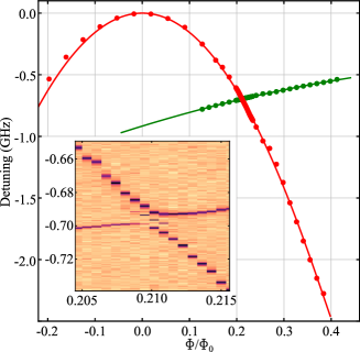
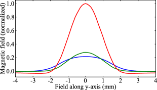
After assessing the functionality of the hose through numerical simulations, we prepared the experiment sup with the aim of verifying the qubit resonance frequency tunability by applying a DC voltage to the coil. In this experiment we use an Arbitrary Waveform Generator (AWG) channel to provide the above mentioned coil excitation. The flux map for both transmon qubits is shown in Fig. 3. The spectroscopy is performed using a saturation pulse with variable frequency, followed by a readout pulse at the cavity resonance frequency, for each value of the AWG output voltage. The maximum applied magnetic field is limited by the coil size and the maximum output voltage of the AWG. The measurement shows that the qubits are tunable as intended. The qubit resonance frequencies are extracted from the measurements and fitted. The flux map also demonstrates the local control capabilities of the hose, as one qubit is more affected by the injected magnetic flux than the other. From the fit we can extract that the hose is around 5 times more effective on the centre qubit, which agrees well with numerical simulations. This factor can be further improved by using an optimised smaller hose design with a funnel-shaped tip and placing the qubits closer to the hose (see Fig. 2).

The data points density has been increased in the avoided crossing region to measure the qubit-qubit interaction, which is $\approx$ 5 MHz. The weak interaction between the qubits is expected from finite element simulations due to the relative qubits distance and position inside the cavity Dalmonte et al. (2015).

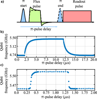
In order to assess the fast flux capabilities of our system, we perform another experiment using the sequence shown in Fig. 4a. To excite the qubit we use a Gaussian amplitude modulated $\pi$-pulse, with a standard deviation of around 70 ns and a total length of 400 ns, generated by the AWG and up-mixed with an IQ-mixer. The $\pi$-pulse length is a trade off between time and frequency resolution for this particular experiment. Another AWG channel is again used to excite the coil, but with pulses added to an optional DC offset. During the measurements, the flux-pulse and the readout pulse have a fixed delay. The frequency and the delay of the $\pi$-pulse are changed linearly, to track the qubit resonance frequency during the flux pulse.

The first measurement (Fig. 4b) is obtained using a square flux-pulse for the coil excitation (dashed line in Fig 4a). In order to avoid ringing effects caused by the AWG, the square pulse’s edges are smoothed by a $\pm\sin(\frac{\pi}{2}\frac{t}{\tau})$ rise or fall for 20 ns, where $\tau=20\,\mathrm{ns}$. The measurement result shows a smooth change of the qubit resonance frequency, with an exponential rise time on the order of 2 $\mu$s. The source of this rise time is still under investigation and is probably caused by eddy currents in the copper clamp holding the hose. A slightly modified clamp design can easily mitigate this effect and will be investigated in future experiments.

In a second set of measurements we speed up the system response through a simple pulse shape, adding an overshoot and an exponential decay (continuous line in Fig. 4b) to the flux pulse. Obtaining the result shown in Fig. 4c, it is evident that now the change in the qubit resonance frequency occurs on time scales $<$ 100 ns. The frequency of the qubit remains stable after around 300 ns without any ringing being evident. The maximum flux step is limited by the maximum available AWG voltage to create the overshoot. A further speed up could be achieved by a proper linear system de-convolution.

Figure 4: Measurements of the qubit tunability with AC magnetic field. (a) Pulse sequence used to perform the fast flux measurements: the Gaussian pulse (blues) is a $\pi$-pulse used to excite the qubit; the flux pulse is shown in green, note that the dashed flux-pulse line is used to get the measurement (b) whereas the continuous line flux pulse is used to get the measurement (c); finally the red pulse is used to readout the qubit state. All the pulses but the $\pi$-pulse are fixed in time, while the frequency and delay of the $\pi$-pulse are linearly changed. The initial position of the pulse defines our time-axis origin and it stops just before the readout pulse, avoiding an overlap. (b) This measurement shows a qubit resonance frequency variation of around 700 MHz. The measured exponential rise time is about 2 $\mu$s. (c) Using the AWG the flux pulse is modified to have an initial overshoot, in order to speed up the rise time that is found in measurement (b). The step size on the time-axis is 20 ns but the resolution given by the $\pi$-pulse is around 50 ns.

After checking the hose capabilities to apply a magnetic field, we estimate the effect of the hose on the system by measuring $T_{1}$, $T_{2}^{*}$, qubit population and the internal quality factor of the cavity. The $T_{1}$ of our qubits is Purcell limited and varies from 15 $\mu$s at the sweet spot to 30 $\mu$s down at 4 GHz. The $T_{2}^{*}$ varies from about 2.2 $\mu$s at the sweet spot, down to 600 ns far from it, with $T_{2E}$ being eight times larger than $T_{2}^{*}$ independent of flux bias. To investigate possible slow frequency noise introduced by the hose, we decided to perform experiments without the hose. For these measurements, we close the hole in the cavity wall and find comparable values for $T_{2}^{*}$ and $T_{2E}$. We believe that the slow frequency noise in the experiments stems from the large SQUID loop and associated flux noise. It is even further aggravated by using the big capacitive shunt pads to close the SQUID loop at the top and bottom Stan et al. (2004); Ithier et al. (2005).

The qubit population has been estimated using the method shown in Geerlings et al. (2013). The result obtained is 80 mK, comparable to the result obtained in the same reference and reference Jin et al. (2015). This result is very typical for our setup and compatible with other experiments done in our lab that do not use hoses.

In order to measure the internal quality factor $Q_{\rm{int}}$ of the cavity with the hose, a reflection measurement using a microwave circulator is done. The measured $Q_{\rm{int}}$ is about $25\cdot 10^{3}$, much less than the expected value in the range of $10^{5}-10^{6}$. Simulations show that this reduction in $Q_{\rm{int}}$ is caused by the fundamental mode’s surface currents being dissipated when they cross the gap between the cavity wall and the hose’s outermost shell Brecht et al. (2015). We experimentally verified this by sealing the gap with indium and measuring again $Q_{\rm{int}}$, reaching $2.75\cdot 10^{5}$. To completely circumvent any lossy seam by introducing the magnetic hose, we suggest to fabricate the outermost shell as part of the cavity when it is machined.

This first magnetic hose design can be improved by a factor of 10 to transfer higher magnetic fields and to act more locally at the qubit’s position sup . Magnetic field transport is enhanced by increasing the layer density, shortening the total length, and elongating all superconducting shells. Addressing can be simply improved by reducing the radius or by forming a funnel-like structure similar to field concentrators Prat-Camps et al. (2013); Zhao et al. (2018). Moreover, it is worth to mention that an optimally designed coil increases the transferred magnetic field.

The maximal amount of magnetic field being transferred through the hose is limited by the used ferromagnetic and superconducting materials. In our setup, fields on the order of $<10^{-6}\,\mathrm{T}$ are sufficient to control the qubits and, thus, materials can be assumed to deviate very little from their ideal linear behaviour. The transfer of much higher fields would induce non-linear responses of the materials, which one would need to analyze carefully. On one hand, the superconducting shells are not expected to significantly limit the hose performance, since radial components of magnetic field (the ones that the superconductor shields) are much smaller than axial components. Furthermore, high-Tc superconductors like YBCO are able to shield magnetic fields of $>$1 T completely Wéra et al. (2017). Ferromagnetic shells, on the other hand, are expected to be the main limiting factor for high-fields transfer. Numerical calculations indicate, though, that fields on the order of hundreds of mT can be transported through hoses made of high-field-saturation ferromagnetic materials like soft irons or electrical steels noa .

The experimental work presented in this paper shows the potential of using a magnetic hose to control various quantum systems. The hose is most applicable in scenario’s where a local applied magnetic field is required, combined with the ability to generate the magnetic field at a distant location and route it to the quantum systems of interest. Most obviously, it would be ideally suited to individually control qubits in superconducting circuits architectures like Zoepfl et al. (2017); Rahamim et al. (2017); Axline et al. (2016) without compromising coherence times. Moreover, due to the ability to apply time varying signals, one could also use the hose to drive parametric amplifiers Mutus et al. (2013, 2014) or tunable couplers Chen et al. (2014). The magnetic hose could also be an ideal candidate to introduce time varying magnetic fields in a hybrid architecture e.g. Rydberg atoms coupled to superconducting microwave cavities Stammeier et al. (2017). The hose might also be applicable to control the magnetic field in gate defined double quantum dots Petta (2005); Stockklauser et al. (2017) or even hybrid scenarios where the quantum dot is coupled to a transmon qubit Scarlino et al. (2018). It could also allow new designs of NMR sensors based on NV centers Arai et al. (2015); Glenn et al. (2018) or even enable magnetic coupling between NV centers Gaebel et al. (2006).

In summary we have shown that a magnetic hose can be used to change the magnetic flux inside an aluminum waveguide cavity in less than 100 ns. The magnetic hose is constructed such that it does no compromise the energy relaxation time of the qubit on the several 10 $\mu$s timescale. Furthermore, the hose can be used to localise the magnetic field and address predominantly one of the qubits inside the cavity. Future improvements to the hose design promise to increase the field transport by a factor of 10 and localize the field to an even smaller volume. As such, the hose is ideally suited to implement fast flux bias lines in 3D Axline et al. (2016) and waveguide Zoepfl et al. (2017) circuit QED architectures.

We gratefully acknowledge fruitful discussions with O. Romero-Isart and thank M.L. Juan and A. Sharafiev for feedback on the paper. Facilities use was supported by the KIT Nanostructure Service Laboratory (NSL). OG and GK are supported by the Austrian Federal Ministry of Education, Science and Research (BMWF), SO und MZ are funded by the European Research Council (ERC) under the European Union’s Horizon 2020 research and innovation program (grant agreement n^∘ 714235). MZ is also supported by the Austrian Science Fund FWF within the DK-ALM (W1259-N27). JPC is funded by the European Research Council (ERC-2013-StG 335489 QSuperMag) and the Austrian Federal Ministry of Education, Science and Research (BMWF).

Supplementary Material

I Setup and measurements

Both transmon qubits are based on an asymmetric SQUID ($d=0.31$) Koch et al. (2007), with a loop size of 200 x 200 $\mu\mathrm{m}^{2}$ and an anharmonicity of 295 MHz. We measured a tunability of more than 3 GHz and maximum frequencies of 6.6 GHz and 6.2 GHz respectively. Below 4 GHz the dispersive shift, the $E_{J}/E_{C}$ ratio and anharmonicity are drastically reduced and it becomes difficult to probe the qubits.

The qubits are capacitively coupled to the first mode of the cavity, with a resonance frequency of 8.102 GHz. The coupling is such that the dispersive shift $\chi\approx$ 5 MHz at the qubit’s maximum transition frequency. The total quality factor of the cavity is limited by the output coupling, engineered to have $\kappa\approx\chi$ at the maximum qubit frequency.

A cryostat input line with a total of 50 dB attenuation and DC - 12 GHz filtering is used to couple to the cavity. A similar line, with only 20 dB of attenuation at the 4 K plate and DC - 80 MHz filtering, is used for driving the coil of the magnetic hose. Additional filtering and better line thermalization is provided by custom-made 50 $\Omega$ absorptive coaxial filters.

To perform a readout, a square, finite-length microwave pulse at the cavity frequency is generated and sent to the system. The signal, transmitted through the cavity, undergoes additional filtering and passes through two isolators, it is then amplified by a HEMT at 4K and by a low noise classical amplifier at room temperature. After that, the signal is down-mixed and digitally recorded by an ADC. Qubit rotations are performed by Gaussian amplitude-modulated pulses generated by an Arbitray Waveform Generator (AWG) and up-converted from around 200 MHz to the qubit frequency. Another AWG channel is used to provide pulsed and DC voltage to the coil, allowing us to reshape the pulses used for the experiment, like described in the main paper.

Figure S1: Simulated magnetic field intensity in x-direction along the y-axis at a distance of 1 mm from the hose for three different hose and coil designs attached to a closed superconducting cavity. The blue line represents the hose used in the paper. The green line considers a hose with higher layer density and elongated shells in combination with a big coil which outer diameter matches the outermost superconducting shell inner diameter. Finally, in red, the maximum improvement is achieved by optimizing both the hose and the coil that magnetizes the ferromagnetic layers in the optimal way.

II Enhancing the magnetic field transport

The magnetic hose presented in the main paper proofs the ability of guiding a magnetic field from the outside to the inside of a superconducting cavity. This first design, however, can be improved to enhance the field transport and to address the magnetic field more locally.

First, the field transport will be enhanced by shortening the total length, increasing the layer density, and elongating all superconducting shells of the magnetic hose on the output side. The length of the inner core can be decreased to minimise the amount of magnetic field leaking and turning back at the cut before entering the cavity. According to Ref. Navau et al. (2014) a higher density of ferromagnetic and superconducting layers increases the magnetic field transport as the metamaterial approaches the ideal material resulting from their calculations. Large densities (layer thickness $\approx 100\,\mathrm{nm}$) and small hose sizes ($\approx 100\,\mathrm{\mu m}$) could be reached with sputtering methods starting from a central ferromagnetic core. Besides the outermost superconducting shell, elongating all superconducting shells will push the magnetic field further into the cavity, since the magnetic field is forced to pass the shells before being routed back. Obviously, elongating the ferromagnetic shells will also enhance the field transport. However, we prefer to have a decent distance between our qubits and the ferromagnet to avoid additional losses for the qubit.

Second, the field distribution at the output side is controlled by the shape of the magnetic hose. By simply reducing the radius of the magnetic hose, the transferred magnetic field is addressed more locally. The addressability is further increased by forming a funnel shaped tip, similar to magnetic field concentrators Prat-Camps et al. (2014). In such a configuration one could transfer and concentrate the field from a large magnetic source at the input side to a tiny spot at the output side of the hose.

Lastly, the design of the coil at the input side of the hose can be optimized to increase the magnetic field transport and to address the magnetic field more locally. It is essential to bring as many turns as possible very close to the metamaterial at the input side of the magnetic hose in order to maximize the magnetic flux injected to the inner ferromagnetic shells. As shown in the simulations, to get magnetic field into the cavity it is necessary that the outer ferromagnetic shells are magnetized in the opposite direction, guiding the magnetic field lines back to the coil. Since the magnetic field strength decreases over the distance, it is more favourable to attach a discoidal coil to the hose instead of a cylindrical coil. Furthermore one should reduce any material counteracting the generated magnetic field to a minimum in the vicinity of the coil. The combined design of the magnetic hose structure and the attached coil is essential for reaching the intended magnetic field distribution at the output side (Fig. S1).

III Shielding properties

Our experiment is surrounded by a copper and a cryoperm shield, providing the usual basic shielding as used in similar experiments Kreikebaum et al. . The bulk aluminum cavity in the superconducting state shields its inside perfectly from external applied magnetic fields, due to the Meissner effect. Introducing a magnetic hose to the cavity opens a link not only for bias fields but also for any external magnetic fields. However, the elongated outermost superconducting shell at the input side provides sufficient shielding from unwanted external magnetic fields. In our experiment we do not see any shift of the flux map recorded on different days within the linewidth of the qubit. Thus, we state sufficient shielding from external magnetic fields and no magnetization of the ferromagnetic material. The coil inside the elongated outermost shell is the only contributor to any frequency shift of both qubits in our experiment. To remove any doubts, one could build a proper superconducting housing at the input side to ensure perfect isolation from external magnetic fields below the critical field of the shield.

In the microwave domain any material with high conductivity reflects microwaves. Thus, microwave shielding is provided fairly easily for instance by a sheet of copper. Since the magnetic hose is a combination of two highly conductive materials, microwaves are expected to be reflected from it. However, one has to introduce a cut to the magnetic hose to guide fast magnetic flux pulses through it. This cut turns out to act as a rectangular waveguide, providing a channel for microwaves to pass through. Due to the height and width of 1.2 mm and 0.4 mm, respectively, the cut-off frequency is above 100 GHz and provides more than 20 dB/mm of attenuation for frequencies below 60 GHz. Similarly, the elongated outermost shell at the input side protects the embedded coil from microwave radiation that could induce a voltage drop leading to flux noise. The outermost shell has an inner diameter of 3 mm and acts as a circular waveguide with a cut-off above 50 GHz resulting in an attenuation larger than 10 dB/mm for frequencies below 20 GHz.

Figure S2: First mode of the bare cavity (8.17 GHz) in isometric (a) and top (b) view. First mode of the cavity with hose (8.23 GHz) in isometric (c) and top (d) view. Fundamental hose mode (10.46 GHz) of the cavity with hose in isometric (e) and top (f) view. The colormap depicts the magnitude of the electric field qualitatively, ranging from blue (minimum) to red (maximum).

IV Effect on cavity modes

Introducing the magnetic hose into the cavity reduces its volume and hence shifts its fundamental mode to a higher frequency compared to a bare cavity of the same size. In addition, the electromagnetic field becomes distorted in the vicinity of the hose to match the condition of zero tangential electrical field along the outermost shell. For that reason the induced currents of a mode inside the cavity do not only flow on the cavity walls, they also have to flow on the outermost shell. The outermost shell effectively becomes part of the cavity and therefore has to be well connected to the cavity wall. Otherwise, currents crossing the gap between the cavity wall and the outermost shell dissipate and limit the internal quality factor of any cavity mode. In that sense one has to consider the orientation of the cut, pointing always in the direction of the electrical field component of the mode of interest. The hose itself acts as a $\lambda/4$-resonator inside the cavity and hence it introduces additional modes depending on its length only, independent of the cavity volume.

In the case of our setup, the first three modes of the bare cavity are at 8.17 GHz, 12.62 GHz. and 13.21 GHz according to finite element simulations. Adding the magnetic hose to the simulations has two effects on the modes inside the cavity. First, in comparison to the bare cavity, a new mode at 10.46 GHz appears. This mode is dominated by the dimensions of the magnetic hose. Second, the cavity-dominated modes are slightly shifted to 8.23 GHz, 12.63 GHz. and 13.20 GHz. The field distribution of selected modes are illustrated in Fig. S2.

Figure S3: Coupling between transmon and cavity in a bare cavity (a) and a cavity with a hose (b). Coupling between two transmons in a bare cavity (c) and a cavity with a hose (d). Anharmonicity of a transmon in a bare cavity (e) and in a cavity with a hose (f). The plots result from finite element simulations. The transmon is moved in half millimeter steps through one quarter of the cavity, where the origin is set at the centre of the cavity. The coupling between two transmons is evaluated by moving both side by side in half millimeter steps, keeping a constant distance of 2 mm between them. The fluctuations of the anharmonicity in (e) and (f) stem from the finite numerical accuracy of the simulations.

V Effect on transmons

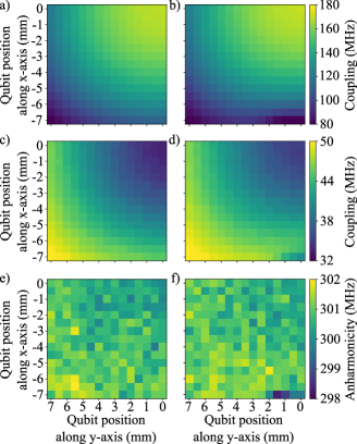
The presence of the magnetic hose does not have any crucial influence on the parameters of the transmon. In the vicinity of $\approx$ 0.5 mm close to the edge of the outermost shell, the capacitive energy of the transmon decreases by $\approx$ 1 % maximally. Thus, its frequency and anharmonicity are affected by the same (negligible) amount. The coupling between the transmon and the cavity is maximally decreased from 113 MHz to 78 MHz, when the transmon is put 0.5 mm close centrally in front of the hose. This is caused by the local deformation of the electromagnetic field in the vicinity of the hose. One can compensate the decreased coupling to the cavity by increasing the total length of the transmon. The coupling between two transmons decreases only if both are closer than 1 mm to the hose in comparison to the bare cavity. Again, this is caused by the local distortion of the electromagnetic field of the transmons and can be compensated by decreasing the distance between them or increasing the pad size. The coupling between the hose mode and the qubit is essentially zero due to symmetry.

References

- Taylor et al. (2008) J. M. Taylor, P. Cappellaro, L. Childress, L. Jiang, D. Budker, P. R. Hemmer, A. Yacoby, R. Walsworth, and M. D. Lukin, Nature Physics 4, 810 (2008).
- Chin et al. (2010) C. Chin, R. Grimm, P. Julienne, and E. Tiesinga, Reviews of Modern Physics 82, 1225 (2010).
- Warring et al. (2013) U. Warring, C. Ospelkaus, Y. Colombe, K. R. Brown, J. M. Amini, M. Carsjens, D. Leibfried, and D. J. Wineland, Physical Review A 87, 013437 (2013).
- Chen et al. (2014) Y. Chen, C. Neill, P. Roushan, N. Leung, M. Fang, R. Barends, J. Kelly, B. Campbell, Z. Chen, B. Chiaro, A. Dunsworth, E. Jeffrey, A. Megrant, J. Y. Mutus, P. J. J. O’Malley, C. M. Quintana, D. Sank, A. Vainsencher, J. Wenner, T. C. White, M. R. Geller, A. N. Cleland, and J. M. Martinis, Physical Review Letters 113, 220502 (2014).
- Yamamoto et al. (2008) T. Yamamoto, K. Inomata, M. Watanabe, K. Matsuba, T. Miyazaki, W. D. Oliver, Y. Nakamura, and J. S. Tsai, Applied Physics Letters 93, 042510 (2008).
- Mutus et al. (2013) J. Y. Mutus, T. C. White, E. Jeffrey, D. Sank, R. Barends, J. Bochmann, Y. Chen, Z. Chen, B. Chiaro, A. Dunsworth, J. Kelly, A. Megrant, C. Neill, P. J. J. O’Malley, P. Roushan, A. Vainsencher, J. Wenner, I. Siddiqi, R. Vijay, A. N. Cleland, and J. M. Martinis, Applied Physics Letters 103, 122602 (2013).
- Caldwell et al. (2018) S. A. Caldwell, N. Didier, C. A. Ryan, E. A. Sete, A. Hudson, P. Karalekas, R. Manenti, M. P. da Silva, R. Sinclair, E. Acala, N. Alidoust, J. Angeles, A. Bestwick, M. Block, B. Bloom, A. Bradley, C. Bui, L. Capelluto, R. Chilcott, J. Cordova, G. Crossman, M. Curtis, S. Deshpande, T. E. Bouayadi, D. Girshovich, S. Hong, K. Kuang, M. Lenihan, T. Manning, A. Marchenkov, J. Marshall, R. Maydra, Y. Mohan, W. O’Brien, C. Osborn, J. Otterbach, A. Papageorge, J.-P. Paquette, M. Pelstring, A. Polloreno, G. Prawiroatmodjo, V. Rawat, M. Reagor, R. Renzas, N. Rubin, D. Russell, M. Rust, D. Scarabelli, M. Scheer, M. Selvanayagam, R. Smith, A. Staley, M. Suska, N. Tezak, D. C. Thompson, T.-W. To, M. Vahidpour, N. Vodrahalli, T. Whyland, K. Yadav, W. Zeng, and C. Rigetti, Physical Review Applied 10, 034050 (2018).
- DiCarlo et al. (2009) L. DiCarlo, J. M. Chow, J. M. Gambetta, L. S. Bishop, B. R. Johnson, D. I. Schuster, J. Majer, A. Blais, L. Frunzio, S. M. Girvin, and R. J. Schoelkopf, Nature 460, 240 (2009).
- Reshitnyk et al. (2016) Y. Reshitnyk, M. Jerger, and A. Fedorov, EPJ Quantum Technology 3, 13 (2016).
- Kong et al. (2015) W.-C. Kong, G.-W. Deng, S.-X. Li, H.-O. Li, G. Cao, M. Xiao, and G.-P. Guo, Review of Scientific Instruments 86, 023108 (2015).
- Navau et al. (2014) C. Navau, J. Prat-Camps, O. Romero-Isart, J. I. Cirac, and A. Sanchez, Physical Review Letters 112, 253901 (2014).
- (12) When a holed superconductor is modelled as a material with a relative permeability , no conditions on the magnetic flux threading the hole are imposed. In our calculations, the zero-flux condition through the hose is imposed by considering the whole closed superconducting cavity. The cavity walls shield the magnetic field in such a way that the total magnetic flux crossing the hole is forced to be zero to fulfil everywhere in space.
- Pendry et al. (2006) J. B. Pendry, D. Schurig, and D. R. Smith, Science 312, 1780 (2006).
- Chen et al. (2010) H. Chen, C. T. Chan, and P. Sheng, Nature Materials 9, 387 (2010).
- Koch et al. (2007) J. Koch, T. M. Yu, J. Gambetta, A. A. Houck, D. I. Schuster, J. Majer, A. Blais, M. H. Devoret, S. M. Girvin, and R. J. Schoelkopf, Physical Review A 76, 042319 (2007).
- (16) See supplementary material
- Dalmonte et al. (2015) M. Dalmonte, S. I. Mirzaei, P. R. Muppalla, D. Marcos, P. Zoller, and G. Kirchmair, Physical Review B 92 (2015), 10.1103/PhysRevB.92.174507.
- Stan et al. (2004) G. Stan, S. B. Field, and J. M. Martinis, Physical Review Letters 92, 097003 (2004).
- Ithier et al. (2005) G. Ithier, E. Collin, P. Joyez, P. J. Meeson, D. Vion, D. Esteve, F. Chiarello, A. Shnirman, Y. Makhlin, J. Schriefl, and G. Schön, Physical Review B 72, 134519 (2005).
- Geerlings et al. (2013) K. Geerlings, Z. Leghtas, I. M. Pop, S. Shankar, L. Frunzio, R. J. Schoelkopf, M. Mirrahimi, and M. H. Devoret, Physical Review Letters 110, 120501 (2013).
- Jin et al. (2015) X. Y. Jin, A. Kamal, A. P. Sears, T. Gudmundsen, D. Hover, J. Miloshi, R. Slattery, F. Yan, J. Yoder, T. P. Orlando, S. Gustavsson, and W. D. Oliver, Physical Review Letters 114 (2015), 10.1103/PhysRevLett.114.240501.
- Brecht et al. (2015) T. Brecht, M. Reagor, Y. Chu, W. Pfaff, C. Wang, L. Frunzio, M. H. Devoret, and R. J. Schoelkopf, Applied Physics Letters 107, 192603 (2015).
- Prat-Camps et al. (2013) J. Prat-Camps, A. Sanchez, and C. Navau, Superconductor Science and Technology 26, 074001 (2013).
- Zhao et al. (2018) P.-F. Zhao, L. Xu, G.-X. Cai, N. Liu, and H.-Y. Chen, Frontiers of Physics 13, 134205 (2018).
- Wéra et al. (2017) L. Wéra, J. Fagnard, D. K. Namburi, Y. Shi, B. Vanderheyden, and P. Vanderbemden, IEEE Transactions on Applied Superconductivity 27, 1 (2017).
- (26) “Magweb | your source of information on magnetic materials,” .
- Zoepfl et al. (2017) D. Zoepfl, P. R. Muppalla, C. M. F. Schneider, S. Kasemann, S. Partel, and G. Kirchmair, AIP Advances 7, 085118 (2017).
- Rahamim et al. (2017) J. Rahamim, T. Behrle, M. J. Peterer, A. Patterson, P. A. Spring, T. Tsunoda, R. Manenti, G. Tancredi, and P. J. Leek, Applied Physics Letters 110, 222602 (2017).
- Axline et al. (2016) C. Axline, M. Reagor, R. Heeres, P. Reinhold, C. Wang, K. Shain, W. Pfaff, Y. Chu, L. Frunzio, and R. J. Schoelkopf, Applied Physics Letters 109, 042601 (2016).
- Mutus et al. (2014) J. Y. Mutus, T. C. White, R. Barends, Y. Chen, Z. Chen, B. Chiaro, A. Dunsworth, E. Jeffrey, J. Kelly, A. Megrant, C. Neill, P. J. J. O’Malley, P. Roushan, D. Sank, A. Vainsencher, J. Wenner, K. M. Sundqvist, A. N. Cleland, and J. M. Martinis, Applied Physics Letters 104, 263513 (2014).
- Stammeier et al. (2017) M. Stammeier, S. Garcia, and A. Wallraff, arXiv:1712.08631 (2017), arXiv:1712.08631 .
- Petta (2005) J. R. Petta, Science 309, 2180 (2005).
- Stockklauser et al. (2017) A. Stockklauser, P. Scarlino, J. V. Koski, S. Gasparinetti, C. K. Andersen, C. Reichl, W. Wegscheider, T. Ihn, K. Ensslin, and A. Wallraff, Physical Review X 7, 011030 (2017).
- Scarlino et al. (2018) P. Scarlino, D. J. van Woerkom, U. C. Mendes, J. V. Koski, A. J. Landig, C. K. Andersen, S. Gasparinetti, C. Reichl, W. Wegscheider, K. Ensslin, T. Ihn, A. Blais, and A. Wallraff, arXiv:1806.10039 (2018), arXiv:1806.10039 .
- Gaebel et al. (2006) T. Gaebel, M. Domhan, I. Popa, C. Wittmann, P. Neumann, F. Jelezko, J. R. Rabeau, N. Stavrias, A. D. Greentree, S. Prawer, J. Meijer, J. Twamley, P. R. Hemmer, and J. Wrachtrup, Nature Physics 2, 408 (2006).
- Arai et al. (2015) K. Arai, C. Belthangady, H. Zhang, N. Bar-Gill, S. J. DeVience, P. Cappellaro, A. Yacoby, and R. L. Walsworth, Nature Nanotechnology 10, 859 (2015).
- Glenn et al. (2018) D. R. Glenn, D. B. Bucher, J. Lee, M. D. Lukin, H. Park, and R. L. Walsworth, Nature 555, 351 (2018).
- Prat-Camps et al. (2014) J. Prat-Camps, C. Navau, and A. Sanchez, Applied Physics Letters 105, 234101 (2014).
- (4) J. M. Kreikebaum, A. Dove, W. Livingston, E. Kim, and I. Siddiqi, 29, 104002, 1608.06273 .